Simulating the formation of molecular clouds. I. Slow formation by gravitational collapse from static initial conditions

Abstract

We study the formation of $\rm{H}_{2}$ in the ISM, using a modified version of the astrophysical magnetohydrodynamical code ZEUS-MP that includes a non-equilibrium treatment of the formation and destruction of $\rm{H}_{2}$. We examine two different approximations to treat the shielding of $\rm{H}_{2}$ against photodissociation: a local approximation, which gives us a solid lower bound on the amount of shielding, and a method based on ray-tracing that is considerably more accurate in some circumstances but that produces results that are harder to clearly interpret. In both cases, the computational cost of determining $\rm{H}_{2}$ photodissociation rates is reduced by enough to make three-dimensional high-resolution simulations of cloud formation feasible with modest computational resources. Our modification to ZEUS-MP also includes a detailed treatment of the thermal behaviour of the gas.

In this paper, we focus on the problem of molecular cloud formation in gravitationally unstable, initially static gas. (In a subsequent paper, we consider turbulent flow). We show that in these conditions, and for initial densities consistent with those observed in the cold, neutral atomic phase of the interstellar medium, $\rm{H}_{2}$ formation occurs on a timescale $t\geq 10\>{\rm Myr}$, comparable to or longer than the gravitational free-fall timescale of the cloud. We also show that the collapsing gas very quickly reaches thermal equilibrium and that the equation of state of the thermal equilibrium gas is generally softer than isothermal.

Finally, we demonstrate that although these results show little sensitivity to variations in most of our simulation parameters, they are highly sensitive to the assumed initial density $n_{\rm i}$. Reducing $n_{\rm i}$ significantly increases the cloud formation timescale and decreases the amount of hydrogen ultimately converted to $\rm{H}_{2}$.

1 Introduction

Since essentially all observed Galactic star formation occurs within dense, self-gravitating molecular clouds, developing an understanding of the origin of these clouds is an important goal of research into star formation. Research in this area has typically focused on trying to answer a few basic questions:

1. How does the molecular gas form? In other words, what are the chemical processes involved?

2. Where does the molecular gas form? Does it form before or after the assembly of the gas into dense clouds?

3. How quickly does the molecular gas form?

By far the largest constituent of the molecular gas is molecular hydrogen, $\rm{H}_{2}$, with other molecules such as ${\rm CO}$ being present only in small amounts, and so in practice the study of the formation of molecular gas is usually simply the study of the formation of $\rm{H}_{2}$.

Although the chemistry of $\rm{H}_{2}$ formation in space remains an active field of study, the basic principles have been understood for some time. Gas-phase formation of $\rm{H}_{2}$ by direct radiative association is highly forbidden and proceeds at a negligible rate, while gas-phase formation via intermediate molecular ions such as $\rm{H}^{-}$ or $\rm{H}_{2}^{+}$ is strongly suppressed by the interstellar radiation field (Glover, 2003) and in any case cannot produce molecular fractions much higher than $x_{\rm{H}_{2}}\simeq 10^{-3}$. Consequently, most Galactic $\rm{H}_{2}$ cannot have formed in the gas phase, leaving grain-surface reactions as the only viable option. The pioneering work of Gould & Salpeter (1963) and Hollenbach & Salpeter (1970, 1971) showed that $\rm{H}_{2}$ molecules could form on the surface of idealized dust grains with an effective rate coefficient compatible with that inferred from UV observations of $\rm{H}_{2}$ in the local interstellar medium, $R_{\rm{H}_{2}}\sim 10^{-17}\>\>{\rm s}^{-1}$ (Jura, 1974). This remains widely accepted, at least for cold dust, although there is ongoing debate about the efficacy of $\rm{H}_{2}$ formation on warm dust (see e.g. Katz et al., 1999; Cazaux & Tielens, 2004).

Answers to the other questions remain far more uncertain. One school of thought argues that $\rm{H}_{2}$ forms in situ, in the locations presently occupied by the observed clouds. According to this picture, gas accumulates due to the action of large scale flows, which may be driven by large-scale gravitational instability (Kennicutt, 1989), magnetic instabilities such as the Parker instability (Parker 1966, although see Kim, Ostriker & Stone 2002 for a recent view of its importance), or may simply be part of the general turbulent velocity field, which itself is probably driven primarily by some combination of energy input from supernovae and from the magnetorotational instability (Mac Low & Klessen, 2004). However, others have argued that the $\rm{H}_{2}$ forms long before the molecular clouds themselves are assembled, residing in the interstellar medium in a diffuse state or in the form of small cloudlets that eventually coalesce to form observable clouds (see Elmegreen 1990 and references therein, or Pringle, Allen & Lubow 2001 for a more recent version of this model). Since coalescence will happen at a much faster rate in regions of converging flow, such as spiral arms, this model can be used to explain the enhanced star formation rates found within spiral arms.

One way to discriminate between these explanations is by determining the ages of observed molecular clouds. If most molecular clouds are young, with ages comparable to their dynamical timescales, then this suggests that they are transient objects, and argues for a dynamical origin. On the other hand, if clouds are old, with lifetimes that are significantly greater than their dynamical timescale, then this is much easier to explain within a model in which clouds build up slowly and are dispersed slowly.

In recent years, evidence that clouds are young has been accumulating. For instance, Ballesteros-Paredes, Hartmann & Vázquez-Semadeni (1999) argue that the absence of post-T Tauri stars with ages greater than $3\>{\rm Myr}$ in the Taurus-Auriga molecular cloud complex implies that the age of this cloud complex can be no more than a few million years. Hartmann, Ballesteros-Paredes & Bergin (2001) elaborate on this idea and show that similarly young ages are implied for most local star-forming regions. Additionally, the age dispersion of stars in open clusters suggests that the molecular cloud complexes that give rise to them must have lifetimes of the order of their dynamical timescales, which are typically no more than a few million years (Elmegreen, 2000). Short cloud lifetimes also make it easier to understand the presence of supersonic magnetohydrodynamical turbulence within the molecular gas: in the absence of forcing, this will decay away within a few turbulent crossing times (Stone, Ostriker & Gammie, 1998; Mac Low, 1999), and so its presence in long-lived clouds requires there to be some form of external or internal driving, whereas its presence in short-lived clouds does not.

Another key piece of evidence for youthful clouds is discussed by Fukui et al. (1999) and Blitz et al. (2006), who show that giant molecular clouds in the Large Magellanic Cloud (LMC) are well-correlated with young stellar clusters, but do not correlate well with older clusters or with supernova remnants. They find that these very large clouds can only last $\sim 6$ Myr before the onset of OB star formation, although they may last another 20 Myr, supported by internal H ii region expansion (e.g. Matzner, 2002; Krumholz, Matzner & McKee, 2006) or external driving by background supernovae (e.g. Joung & Mac Low, 2006), before their final dissolution by the same agents.

However, for a model involving rapid cloud formation to be viable, it must be possible to produce the required quantity of $\rm{H}_{2}$ within a few million years. Given the relatively slow rate at which $\rm{H}_{2}$ forms, it is natural to ask whether it is possible to satisfy this requirement. Simple back-of-the-envelope estimates made using the $\rm{H}_{2}$ formation rate quoted above suggest that it is possible, provided that the mean density of the material making up the cloud exceeds $10^{3}\>{\rm cm}^{-3}$ (Hartmann, Ballesteros-Paredes & Bergin, 2001), but we would ideally like to be able to confirm this result with more detailed numerical modeling. Various efforts in this direction have been made by a number of groups (Hennebelle & Pérault, 1999, 2000; Koyama & Inutsuka, 2000, 2002; Bergin et al., 2004), but to date this modeling has generally been restricted to one or two dimensions, and has assumed an initially ordered, large-scale velocity field, such as a convergent flow, despite the observational evidence that the velocity field of the neutral interstellar medium (ISM) is dominated by disordered, turbulent motions (see e.g. Lazarian & Pogosyan, 2000).

On the other hand, existing three-dimensional simulations of the neutral ISM, which do properly treat the velocity field and often also include an approximate treatment of the thermal balance of the gas (e.g. Korpi et al. 1999; de Avillez 2000; Wada 2001; Kritsuk & Norman 2002a,b, 2004; Balsara et al. 2004; de Avillez & Breitschwerdt 2004; Slyz et al. 2005; Joung & Mac Low 2006) have not previously included sufficient chemistry to follow the formation of $\rm{H}_{2}$ and so have been unable to directly address the questions posed here.

To bridge this gap, we have performed simulations of the neutral ISM using a hydrodynamical code capable of following both the thermal balance of the gas and the formation and destruction of $\rm{H}_{2}$ within it. Our goal is to determine how quickly significant quantities of $\rm{H}_{2}$ can form in the dense neutral ISM, and to use this information to assess whether models in which cloud formation is assumed to be rapid are likely to work in practice. In this paper, we discuss in detail the numerical method used to follow the coupled chemical, thermal and dynamical evolution of the gas, and the tests used to verify the correctness of our implementation. We also present results from an application of our method to the problem of $\rm{H}_{2}$ formation in gas that is gravitationally unstable, but not turbulent. In a companion paper (Glover & Mac Low 2006; hereafter, paper II) we present results from a large suite of simulations that include the effects of supersonic turbulence. Although highly simplified, and probably not representative of real clouds, the non-turbulent models examined in the second half of the present paper allow us to place an upper limit on the time required to form a molecular cloud, given neutral atomic gas with the density assumed in our initial conditions. By comparing the results of these simulations with the results from the turbulent models examined in paper II, we can more clearly identify the effects of the turbulence, allowing us to demonstrate that supersonic turbulence significantly reduces the time required to form large quantities of $\rm{H}_{2}$.

The structure of the current paper is as follows. In § 2 we describe the methods used to solve the equations of fluid flow, with a focus on our treatment of the thermal and chemical evolution of the gas, and in § 3 we present the results of some basic tests of our approach. In § 4, we describe and motivate the initial conditions used for our simulations. In § 5, we present results from simulations of gravitationally unstable gas which is initially at rest, paying particular attention to the rate of $\rm{H}_{2}$ formation and the spatial distribution of the resulting molecular gas. Finally, in § 6 we summarize our main results.

2 Numerical method

2.1 Magnetohydrodynamical equations

The governing equations for the flow of an inviscid, magnetized, self-gravitating gas can be written as (Stone & Norman, 1992b):

$$\frac{{\rm D}\rho}{{\rm D}t}=-\rho\nabla\cdot\mbox{\boldmath{$v$}},$$ (1)

$$\rho\frac{{\rm D}\mbox{\boldmath{$v$}}}{{\rm D}t}=-\nabla p-\rho\nabla\Phi+\frac{1}{4\pi}(\nabla\times\mbox{\boldmath{$B$}})\times\mbox{\boldmath{$B$}},$$ (2)

$$\rho\frac{{\rm D}}{{\rm D}t}\left(\frac{e}{\rho}\right)=-p\nabla\cdot\mbox{\boldmath{$v$}}-\Lambda,$$ (3)

$$\frac{\partial\mbox{\boldmath{$B$}}}{\partial t}=\nabla\times(\mbox{\boldmath{$v$}}\times\mbox{\boldmath{$B$}}),$$ (4)

$$\nabla^{2}\Phi=4\pi G\rho,$$ (5)

where $\rho$ $e$, $p$, $v$, $B$ and $\Phi$ are, respectively, the mass density, internal energy density, pressure, velocity, magnetic field and gravitational potential of the gas, where ${\rm D}/{\rm D}t$ denotes the comoving derivative

$$\frac{{\rm D}}{{\rm D}t}=\frac{\partial}{\partial t}+\mbox{\boldmath{$v$}}\cdot\nabla,$$ (6)

and where $\Lambda$ denotes the net rate at which the gas gains or loses internal energy due to radiative and chemical heating and cooling. Additionally, in a chemically reactive flow, each chemical species satisfies an equation of the form

$$\frac{{\rm D}\rho_{i}}{{\rm D}t}=-\rho_{i}\nabla\cdot\mbox{\boldmath{$v$}}+{\rm C}_{i}-{\rm D}_{i},$$ (7)

where $\rho_{i}$ is the mass density of species $i$, and where ${\rm C}_{i}$ and ${\rm D}_{i}$ represent its creation and destruction by chemical reactions. Finally, to close the set of equations, it is necessary to specify an equation of state relating the internal energy and the pressure. For an ideal gas we can write this as

$$p=(\gamma-1)e,$$ (8)

where $\gamma$, the ratio of specific heats, depends upon the composition of the gas. For a gas with a number density $n$ of hydrogen nuclei, a number density $n_{\rm{He}}=0.1n$ of helium nuclei, and with a molecular hydrogen abundance $x_{\rm{H}_{2}}=2n_{\rm{H}_{2}}/n$ and an electron abundance $x_{\rm{e}}=n_{\rm{e}}/n$, we can write $\gamma$ as

$$\gamma=\frac{5.5+5x_{\rm{e}}-1.5x_{\rm{H}_{2}}}{3.3+3x_{\rm{e}}-0.5x_{\rm{H}_{2}}},$$ (9)

where we have assumed that the rotational degrees of freedom of $\rm{H}_{2}$ are populated, but that the vibrational degrees of freedom are not. With the definition of $x_{\rm{H}_{2}}$ that we have adopted here, a value of $x_{\rm{H}_{2}}=1.0$ corresponds to gas in which all of the hydrogen is in molecular form, in which case $\gamma=10/7$. (Note that the more familiar $\gamma=7/5$ is for a gas which is pure $\rm{H}_{2}$; the presence of the helium in our simulations causes a slight hardening of the equation of state).

To solve this set of equations, we used a modified version of the publicly available ZEUS-MP hydrodynamical code. ZEUS-MP is a multi-physics, massively-parallel, message-passing code for astrophysical fluid dynamics (Norman, 2000), developed by the Laboratory for Computational Astrophysics at UC San Diego, which solves the equations of self-gravitating magnetohydrodynamics (MHD) in three dimensions. The algorithms used in the ZEUS family of hydrocodes are described in detail in Stone & Norman (1992a,b) and Hawley & Stone (1995). Their implementation within ZEUS-MP is discussed in Fiedler (1997) and Norman (2000). The Poisson solver used is a Fourier space solver that utilizes the FFTW library (Frigo & Johnson, 1998). Our modified version of ZEUS-MP is derived from version 1.0b of the code. (For details of the more recently released version 2, see Hayes et al. 2006).

We have modified ZEUS-MP in two main respects. Firstly, in order to follow non-equilibrium chemistry within the gas it is necessary to add an extra field variable for each chemical species that we wish to track. A natural choice of variable is the mass density of each species, as in that case in a medium with $N$ non-equilibrium chemical species, we will have $N$ equations of the form of equation 7 to solve. As discussed below in § 2.2, we follow only two non-equilibrium species in the simulations presented here – $\rm{H}_{2}$ and $\rm{H}^{+}$ – and so have two such equations to solve. To solve these equations, we use operator splitting to separate the effects of advection (which is treated in the same fashion as advection of the total mass density; see Stone & Norman 1992a) from those of the chemical creation and destruction terms. In other words, during the reaction step we solve the equations

$$\frac{\partial\rho_{\rm{H}_{2}}}{\partial t} = {\rm C}_{\rm{H}_{2}}(\rho_{\rm{H}_{2}},\rho_{\rm{H}^{+}},T)-{\rm D}_{\rm{H}_{2}}(\rho_{\rm{H}_{2}},\rho_{\rm{H}^{+}},T),$$ (10)

$$\frac{\partial\rho_{\rm{H}^{+}}}{\partial t} = {\rm C}_{\rm{H}^{+}}(\rho_{\rm{H}_{2}},\rho_{\rm{H}^{+}},T)-{\rm D}_{\rm{H}^{+}}(\rho_{\rm{H}_{2}},\rho_{\rm{H}^{+}},T).$$ (11)

The method of solution that we adopt is implicit finite differencing: we approximate equations 10 & 11 as

$$\rho_{\rm{H}_{2}}^{i+1} = \rho_{\rm{H}_{2}}^{i}+\Delta t\left[{\rm C}_{\rm\rm{H}_{2}}^{i+1}-{\rm D}_{\rm\rm{H}_{2}}^{i+1}\right],$$ (12)

$$\rho_{\rm{H}^{+}}^{i+1} = \rho_{\rm{H}^{+}}^{i}+\Delta t\left[{\rm C}_{\rm\rm{H}^{+}}^{i+1}-{\rm D}_{\rm\rm{H}^{+}}^{i+1}\right],$$ (13)

where the superscripts indicate values at the beginning and end of the timestep. The advantage of using a first-order implicit method is that we can guarantee that the abundances will remain non-negative and that the solution will remain stable regardless of the size of the timestep chosen (although the requirement that we solve equations 12 & 13 accurately still places some limits on the size of the timestep). The disadvantage of using an implicit method is that the resulting finite difference equations are coupled and must be solved iteratively. Moreover, the fact that the creation and destruction terms also depend strongly on the internal energy of the gas (through the temperature $T$) suggests that we should solve these equations simultaneously with the energy equation. We therefore defer discussion of the solution of equations 12 & 13 until after we have discussed the modifications that we have made to the treatment of the internal energy equation.

This has been modified to include a term representing the combined effects of radiative and chemical heating or cooling, i.e. the $\Lambda$ term of equation 3. Details of the processes included are given in § 2.3 below and are summarized in Table 2. Solution of the resulting equation proceeds much as it does in the unmodified version of ZEUS-MP: the equation is operator split, with the effects of artificial viscosity, compressional heating and advection treated separately. Our treatment of the artificial viscosity and advection steps mirrors that in the unmodified version of the code, as discussed in detail in Stone & Norman (1992a); we will not discuss it here. However, during the compressional heating step, instead of solving the equation

$$\frac{\partial e}{\partial t}=-p\nabla\cdot\mbox{\boldmath{$v$}},$$ (14)

we solve

$$\frac{\partial e}{\partial t}=-p\nabla\cdot\mbox{\boldmath{$v$}}-\Lambda.$$ (15)

To solve equation 15, we use an algorithm based on a combination of the ZEUS-3D pdvcool algorithm (originally implemented by M. Norman and subsequently modified by M.-M. Mac Low, J. Stone and D. Clarke) with the implicit algorithm used by Suttner et al. (1997) and further developed by Pavlovski et al. (2002) and Smith & Rosen (2003). We construct the following implicit approximation to equation 15

$$\frac{e^{i+1}-e^{i}}{\Delta t}=-\tilde{p}\nabla\cdot\mbox{\boldmath{$v$}}^{i}-\Lambda^{i+1},$$ (16)

where $\tilde{p}$ represents the time-centered pressure, which we approximate as $\tilde{p}\simeq 0.5[p(e^{i+1})+p(e^{i})]$, and where $\Lambda^{i+1}$ is the cooling rate at the end of the timestep. We rearrange this equation to give

$$e^{i+1}=\frac{(1-q)e^{i}-\Lambda^{i+1}\Delta t}{1+q},$$ (17)

where

$$q=\frac{\Delta t}{2}(\gamma-1)(\nabla\cdot\mbox{\boldmath{$v$}}^{i}),$$ (18)

and then solve equation 17 together with equations 12 & 13 using a form of Gauss-Seidel iteration. This works as follows:

1. Update $\rho_{\rm{H}_{2}}$, using old values for $\rho_{\rm{H}^{+}}$ and $e$.

2. Update $\rho_{\rm{H}^{+}}$, using new value for $\rho_{\rm{H}_{2}}$ but old value for $e$.

3. Update $e$, using new values for $\rho_{\rm{H}_{2}}$ and $\rho_{\rm{H}^{+}}$.

4. Test for convergence. If not converged, return to step 1.

On our first pass through the loop, we take the old values for $\rho_{\rm{H}^{+}}$ and $e$ to be those at the start of the current timestep. On subsequent passes through the loop, we instead use the values from the previous iteration.

Since the internal energy converges more slowly than either of the chemical abundances, we monitor its value to determine when to stop the iteration, halting once the relative difference between updated and old values becomes less than $10^{-7}$. On rare occasions, the iteration may fail to converge. In this case, we switch to solving for $e$ using a more expensive bisection algorithm that is sure to find a solution. In this case, we lose the benefits of the iteration for refining our initial guesses for $\rho_{\rm{H}_{2}}$ and $\rho_{\rm{H}^{+}}$. Fortunately, the abundances of $\rm{H}_{2}$ and $\rm{H}^{+}$ generally do not vary much during a single timestep and so the error that this introduces is probably not significant, particularly since the iteration almost always succeeds.

To compute the cooling timestep, $\Delta t_{\rm cool}$, we use the same procedure as in Suttner et al. (1997) and Pavlovski et al. (2002): we compute $\Lambda$ and then require that the timestep be such that the internal energy will not vary by more than 30% given this value of $\Lambda$, i.e.

$$\Delta t_{\rm cool}=0.3\frac{e}{|\Lambda|}.$$ (19)

To improve the efficiency of the code, we also make use of subcycling. Rather than constraining the global timestep of the simulation $\Delta t$ to be less than $\Delta t_{\rm cool}$, we instead use the same global timestep as we would within the unmodified version of the code, but solve the chemistry and cooling substeps alone over the shorter cooling timescale, repeating the procedure for as many times as is necessary to make the total elapsed time equal to $\Delta t$. Thus, if $\Delta t_{\rm cool}\geq\Delta t$, we proceed through the chemistry and cooling substep only once per simulation timestep, while if $\Delta t_{\rm cool}\ll\Delta t$, we do so many times, using the updated values of the chemical abundances and internal energy from the end of one substep as the input to the next. We subcycle at the level of the individual grid zones, so only zones for which $\Delta t_{\rm cool}<\Delta t$ take multiple chemistry and cooling substeps per hydrodynamical timestep. The gain in computational efficiency from this subcycling procedure is difficult to quantify, as it depends on the physical state of the gas, but tests indicate that it can easily be as much as an order of magnitude.

2.2 Chemistry

The chemical composition of the ISM is complex. Over 120 different molecular species have been detected in interstellar space (Wiklind, 2004) and while many of these are found in detectable amounts only in dense, well-shielded gas, there remain a significant number that have been detected in diffuse, unshielded gas (see, for instance O’Neill, Viti & Williams, 2002, and references therein). A full chemical model of the ISM can easily involve several hundred different atomic and molecular species and several thousand different reactions, even if reactions on grain surfaces are neglected (e.g. Le Teuff, Millar & Markwick, 2000).

It is currently impractical to incorporate this amount of chemistry into a 3D hydrodynamical code such as ZEUS-MP, due to the extreme impact it would have on the code’s performance. Fortunately, much of this chemistry is not relevant to our current study, and can be neglected without significantly compromising our results. Recall that the main goals of this paper are to determine the timescale on which molecular clouds form in gravitationally unstable atomic gas, and the fraction of this gas that is converted to molecular form. To achieve these goals, we clearly need to be able to follow the formation and destruction of $\rm{H}_{2}$ with a reasonable degree of accuracy. Beyond this, however, the only chemistry that we really need to be concerned with is that which plays a role in determining the thermal balance of the gas. In other words, we need only follow the chemistry of $\rm{H}_{2}$, and of a few other major coolants such as ${\rm C}^{+}$ or ${\rm O}$; the chemistry of other molecules such as ${\rm CH}$, while undeniably of interest, is not central to the task at hand and so can be sacrificed in pursuit of efficiency.

To identify the major coolants in the diffuse ISM, we can use the results of Wolfire et al. (1995, 2003), who studied its thermal evolution in some detail. They show that in the warm neutral medium (WNM), which has a characteristic temperature $T\sim 8000\>{\rm K}$, most of the cooling comes from Lyman-$\alpha$ emission from atomic hydrogen, electron recombination with small grains and polycyclic aromatic hydrocarbons (PAHs), and fine structure emission from atomic oxygen. Cooling in the cold neutral medium (CNM), which has a characteristic temperature $T<300\>{\rm K}$, is dominated by fine structure emission from ionized carbon, C ii , with fine structure emission from oxygen also contributing significantly in the warmer parts of the CNM. These two coolants also dominate in the thermally unstable temperature regime $300<T<8000\>{\rm K}$. Heating in all three regimes is dominated by photoelectric emission from dust grains and PAHs; the heating rate is therefore primarily determined by the strength of the ultraviolet background and by the dust to gas ratio, but it also has a dependence on the electron abundance (see equation 43 in § 2.3). We also include fine structure cooling from ${\rm Si^{+}}$. Although never the dominant coolant, ${\rm Si^{+}}$ does produce $\sim 10\%$ of the total fine structure emission at temperatures $T>200\>{\rm K}$ at all densities, and can produce as much as 30% of the emission at high densities, owing to the relatively large size of Einstein coefficient for the ${\rm Si^{+}}$ ${}^{2}P_{3/2}\rightarrow^{2}P_{1/2}$ transition (Silva & Viegas, 2002).

In denser gas that is shielded from the ultraviolet background, other coolants such as ${\rm CO}$ and ${\rm H_{2}O}$ become important, as demonstrated by Goldsmith & Langer (1978), Neufeld & Kaufman (1993) and Neufeld, Lepp & Melnick (1995). However, since we are primarily interested in the transition from atomic to molecular gas, and since these coolants will not become important until after the gas is already fully molecular, we have chosen to make another major simplification in the chemistry: we assume that carbon, oxygen and silicon remain primarily in the form of C ii , O i and Si ii respectively, throughout the simulation. By making this assumption, we essentially reduce the chemistry that must be followed to that of only three species – electrons, neutral hydrogen and $\rm{H}_{2}$ – at the cost of computing an incorrect cooling rate in dense molecular gas. The dense gas in our simulations is also typically rather cold, with a temperature of no more than a few tens of Kelvin, and so we will probably underestimate the cooling rate within it, since in these conditions molecular coolants such as ${\rm CO}$ are more effective than the C ii , O i and Si ii included in our simulations. This means that we probably overestimate the temperature of this gas, but the fact that the dense gas is so cold shows that we do not overestimate its temperature by a large amount, and we therefore do not expect this approximation to have a significant impact on the $\rm{H}_{2}$ formation rate.

Having discussed the underlying assumptions, we now present our chemical model. We adopt standard solar abundances of hydrogen and helium, along with abundances of carbon, oxygen and silicon taken from Sembach et al. (2000): $x_{\rm C}=1.4\times 10^{-4}$, $x_{\rm O}=3.2\times 10^{-4}$, $x_{\rm Si}=1.5\times 10^{-5}$. We assume that helium remains neutral and plays no direct role in the chemistry, and that carbon and silicon remain singly ionized throughout the simulation. The ionization state of oxygen is assumed to track that of hydrogen, due to the influence of the charge transfer reactions

$${\rm O}^{+}+\rm{H} \rightarrow {\rm O}+\rm{H}^{+},$$ (20)

$$\rm{H}^{+}+{\rm O} \rightarrow \rm{H}+{\rm O^{+}}.$$ (21)

As previously noted in § 2.1, we follow directly the abundances of two chemical species, namely $\rm{H}^{+}$ and $\rm{H}_{2}$. The abundances of the other major species – atomic hydrogen and electrons – are computed from the conservation laws:

$$x_{\rm{H}}=x_{\rm H,tot}-x_{\rm{H}^{+}}-x_{\rm{H}_{2}},$$ (22)

and

$$x_{\rm{e}}=x_{\rm{H}^{+}}+x_{\rm C^{+}}+x_{\rm Si^{+}},$$ (23)

where $x_{\rm H,tot}$ is the total abundance of hydrogen nuclei, in all forms, and where $x_{\rm C^{+}}$ and $x_{\rm Si^{+}}$ represent the abundances of ionized carbon and silicon respectively. We neglect the small contributions to $x_{\rm{e}}$ made by electrons from other ionized metals, such as ${\rm Mg}$ or ${\rm S}$, since these are small compared to the contribution from carbon. We also neglect any contribution from ${\rm O^{+}}$, as this will be negligible compared to the contribution from hydrogen.

Our assumption that carbon and silicon remain ionized throughout the simulation becomes inaccurate in dense, well-shielded gas, where UV photoionization of neutral carbon and silicon becomes ineffective. We therefore overestimate the fractional ionization of gas in these regions. However, our main motivation for tracking the fractional ionization is to compute the photoelectric heating rate accurately, and since this is unimportant in dense, shielded gas, the inaccuracy in the fractional ionization is likely unimportant there.

The reactions included in our chemical model are summarized in Table 1. In most cases, we also list the source or sources from which we took the rate coefficient used in our model. The exception is $\rm{H}_{2}$ photodissociation, the treatment of which is discussed in detail in § 2.2.1 below. Two other reactions deserve further comment: the collisional dissociation of $\rm{H}_{2}$ by atomic hydrogen

$$\rm{H}_{2}+\rm{H}\rightarrow 3\rm{H},$$ (24)

and molecular hydrogen

$$\rm{H}_{2}+\rm{H}_{2}\rightarrow\rm{H}_{2}+2\rm{H}.$$ (25)

The reaction coefficients for both of these reactions are density-dependent, since they are sensitive to the population of the vibrational and rotational levels of $\rm{H}_{2}$. To treat the former, we use a rate coefficient

$$\log k_{\rm{H}}=\left(\frac{n/n_{\rm cr}}{1+n/n_{\rm cr}}\right)\log k_{\rm\rm{H},h}+\left(\frac{1}{1+n/n_{\rm cr}}\right)\log k_{\rm\rm{H},l},$$ (26)

where $k_{\rm\rm{H},l}$ is the low density limit of the collisional dissociation rate and is taken from Mac Low & Shull (1986), while $k_{\rm\rm{H},h}$ is the high density limit, taken from Lepp & Shull (1983). The critical density, $n_{\rm cr}$, is given by

$$\frac{1}{n_{\rm cr}}=\frac{x_{\rm{H}}}{n_{\rm cr,\rm{H}}}+\frac{x_{\rm{H}_{2}}}{n_{\rm cr,\rm{H}_{2}}},$$ (27)

where $n_{\rm cr,\rm{H}}$ and $n_{\rm cr,\rm{H}_{2}}$ are the critical densities in pure atomic gas with an infinitesimally dilute quantity of $\rm{H}_{2}$ and in pure molecular gas respectively. The first of these values is taken from Lepp & Shull (1983), but has been decreased by an order of magnitude, as recommended by Martin, Schwarz & Mandy (1996); the other value comes from Shapiro & Kang (1987). To treat the collisional dissociation of $\rm{H}_{2}$ by $\rm{H}_{2}$ we use a similar expression

$$\log k_{\rm{H}_{2}}=\left(\frac{n/n_{\rm cr}}{1+n/n_{\rm cr}}\right)\log k_{\rm\rm{H}_{2},h}+\left(\frac{1}{1+n/n_{\rm cr}}\right)\log k_{\rm\rm{H}_{2},l},$$ (28)

where the low density limit, $k_{\rm\rm{H}_{2},l}$, is taken from Martin, Keogh & Mandy (1998) and the high density limit, $k_{\rm\rm{H}_{2},h}$, is taken from Shapiro & Kang (1987). The collisional dissociation rates computed in this way are acceptably accurate when $n_{\rm{H}}\gg n_{\rm{H}_{2}}$ or $n_{\rm{H}}\ll n_{\rm{H}_{2}}$, but may be less accurate in gas with $n_{\rm{H}}\sim n_{\rm{H}_{2}}$; further study of the collisional dissociation of $\rm{H}_{2}$ in gas which is a mixture of $\rm{H}$ and $\rm{H}_{2}$ would be desirable to help remedy this.

We do not include the gas phase formation of $\rm{H}_{2}$ via the $\rm{H}^{-}$ or $\rm{H}_{2}^{+}$ ions, as in the typical conditions of the Galactic ISM, this is unimportant compared to the formation of $\rm{H}_{2}$ on dust grains (Glover, 2003).

As can be seen from Table 1, our $\rm{H}^{+}$ chemistry is straightforward. However, a couple of reactions are deserving of comment. One is gas-phase recombination, where we note that we use the case B value for the recombination coefficient, as this is the most appropriate choice in all but the most highly ionized gas. The other is the cosmic ray ionization of $\rm{H}$. In the majority of our simulations, we use a value of the cosmic ray ionization rate $\zeta=10^{-17}\>{\rm s^{-1}}$. This is consistent (within the error bars) with recent determinations of the ionization rate in dense cores within molecular clouds (Caselli et al., 1998; Bergin et al., 1999; van der Tak & van Dishoeck, 2000). However, measurements of the ${\rm H_{3}^{+}}$ column density along sight-lines passing through diffuse gas are only explained by a much larger value of $\zeta$, within the range $10^{-16}<\zeta<10^{-15}\>{\rm s^{-1}}$ (McCall et al., 2003; Liszt, 2003; Le Petit, Roueff & Herbst, 2004), where the uncertainty is due primarily to the uncertain distribution of gas along the observed lines of sight. The cause of this discrepancy is currently unknown (although Padoan & Scalo 2005 suggest one possible mechanism), and so for simplicity we take $\zeta$ to be constant, independent of the gas density. We briefly examine in § 5.4 the consequences of adopting a larger value for $\zeta$.

2.2.1 $\rm{H}_{2}$ photodissociation

Following Draine & Bertoldi (1996), we can write the photodissociation rate of $\rm{H}_{2}$ in optically thin gas as

$$k_{\rm ph,0}=3.3\times 10^{-11}\chi\>\>{\rm s}^{-1},$$ (29)

where we have assumed that the ultraviolet field has the same spectral shape as the Draine (1978) field, and where $\chi$ is a dimensionless factor which characterizes the intensity of the field at $1000\>$Å relative to the Habing (1968) field; note that for the original Draine (1978) field, $\chi=1.7$.

By balancing this dissociation rate against the rate at which $\rm{H}_{2}$ forms on dust grains, we can easily show that the equilibrium $\rm{H}_{2}$ fraction in cold gas is given by

$$x_{\rm{H}_{2}}\sim 10^{-6}\chi^{-1}\left(\frac{T}{100}\right)^{1/2}n_{\rm{H}},$$ (30)

which is clearly far less than one unless $n_{\rm{H}}$ is very large. Since observations indicate that significant molecular gas is present at densities below $n_{\rm{H}_{2}}<10^{4}\>{\rm cm}^{-3}$ (see e.g. Falgarone et al., 1998), it is clear that some shielding of interstellar $\rm{H}_{2}$ molecules from the effects of UV photodissociation must occur, and that simulations of molecular cloud formation which do not take this shielding into account are going to be tremendously inaccurate.

$\rm{H}_{2}$ can be shielded against photodissociation in two main ways: by line absorption due to other $\rm{H}_{2}$ molecules (i.e. self-shielding), and by continuous absorption due to dust. The effects of both processes have been treated in some detail by Draine & Bertoldi (1996). They show that in shielded gas the photodissociation rate can be written approximately as

$$k_{\rm ph}=f_{\rm shield}(N_{\rm{H}_{2}})e^{-\tau_{\rm d,1000}}k_{\rm ph,0},$$ (31)

where $f_{\rm shield}$ is a numerical factor accounting for the effects of self-shielding, $\tau_{\rm d,1000}$ is the optical depth due to dust at $1000$Å, and $k_{\rm ph,0}$ is the unshielded photodissociation rate, given by equation 29 above.

Draine & Bertoldi show that for a static, plane parallel slab of gas, $f_{\rm shield}$ is well approximated by

$$f_{\rm shield}=\frac{0.965}{(1+x/b_{5})^{2}}+\frac{0.035}{(1+x)^{1/2}}\exp\left[-8.5\times 10^{-4}(1+x)^{1/2}\right],$$ (32)

where $x=N_{\rm{H}_{2}}/5\times 10^{14}\>{\rm cm}^{-2}$ with $N_{\rm{H}_{2}}$ being the $\rm{H}_{2}$ column density, and $b_{5}=b/10^{5}\>{\rm cm}\>{\rm s}^{-1}$, where $b$ is the Doppler broadening parameter.

If the gas is not static or in uniform motion, but instead has a spatially varying velocity, then equation 32 will overestimate the amount of self-shielding that occurs. The reason for this is that if the velocity field is non-uniform, then the relative velocity between any two fluid elements will, in general, be non-zero. Consequently, the contribution to the total absorption coming from the first fluid element will be Doppler shifted when viewed from the rest frame of the second fluid element. If this Doppler shift is large compared to the line widths of the Lyman-Werner band transitions, then the effect is to significantly reduce the extent to which the absorption coming from the first fluid element contributes to the self-shielding seen by the second fluid element. For $\rm{H}_{2}$ column densities $N_{\rm{H}_{2}}<10^{17}\>{\rm cm^{-2}}$, the intrinsic widths of even the strongest Lyman-Werner band transitions are unimportant and the line profiles are dominated by Doppler broadening. In this regime, the neglect of changes in the velocity along the line of sight is justified if the differences in velocity are much smaller than the sound speed of the gas, and equation 32 remains a good estimator for $f_{\rm shield}$. On the other hand, if the differences in the velocity are much greater than the sound speed, as will generally be the case in a supersonically turbulent flow, then equation 32 will significantly overestimate the degree of self-shielding that will actually occur.

For $N_{\rm{H}_{2}}>10^{17}\>{\rm cm^{-2}}$, the line widths of the strongest transitions are dominated by Lorentz broadening, and the degree of self-shielding in these lines becomes insensitive to the velocity distribution of the gas, unless the range of velocities is extremely large. However, the total $\rm{H}_{2}$ photodissociation rate remains sensitive to the velocity dispersion, as a large fraction of the total rate is due to absorption in weaker lines, whose widths are still dominated by Doppler broadening. Only for $N_{\rm{H}_{2}}>10^{18}\>{\rm cm^{-2}}$ does the total photodissociation rate become relatively insensitive to the velocity distribution of the gas.

An additional problem with using equation 32 to compute the self-shielding factor is that it requires us to compute the $\rm{H}_{2}$ column densities along a large number of lines of sight for every zone in our simulation. Unfortunately, the computational cost of doing so is very large: for a simulation with $N$ fluid elements, the cost of solving for the column densities scales as $O(N^{5/3})$ (assuming that we require an angular resolution that is well matched with the spatial resolution of the code), compared to scalings of $O(N)$ for the hydrodynamical algorithms and $O(N\log N)$ for the self-gravity. Consequently, solving for the column densities would quickly come to dominate the cost of the simulation, and would prevent us from performing any high resolution simulations. Moreover, while parallelization of the code would help to some extent, efficient parallelization of the radiative transfer is difficult, owing to the way in which it couples together widely separated regions in the computational volume.

Computation of the optical depth due to dust, $\tau_{\rm d,1000}$, is in principle considerably simpler than computation of $f_{\rm shield}$, since it involves continuous absorption rather than line absorption, and so Doppler effects can generally be neglected (at least for the velocities of interest here). Cardelli, Clayton & Mathis (1989) showed that it is possible to approximate the extinction observed along many lines of sight in the Galaxy by a one-parameter family of curves, where the controlling parameter is $R_{V}$, defined as

$$R_{V}=\frac{A_{V}}{A_{B}-A_{V}},$$ (33)

where $A_{B}$ and $A_{V}$ are the extinctions in the B and V bands respectively. For $R_{V}=3.1$, which is typical for many lines of sight in the diffuse ISM, Draine & Bertoldi (1996) quote an effective attenuation cross-section for the dust of $\sigma_{\rm d,1000}=2\times 10^{-21}\>{\rm cm^{2}}$. The corresponding dust opacity is given by

$$\tau_{\rm d,1000}=2\times 10^{-21}N_{\rm\rm{H},tot},$$ (34)

where $N_{\rm\rm{H},tot}=N_{\rm{H}}+N_{\rm{H}^{+}}+2N_{\rm{H}_{2}}$ is the total column density of hydrogen nuclei between the point of interest and the source of the radiation. Therefore, to compute the effects of the dust shielding, we again need to compute appropriate column densities, although in this case the effect of velocity differences along the line of sight is unimportant. As in the case of self-shielding, the cost of solving for the column densities is $O(N^{5/3})$ for a simulation with $N$ fluid elements, and so a high resolution treatment of both the fluid flow and the radiation field is not computationally feasible.

To overcome these difficulties, we have performed simulations using two different approximations. Our first approximation is very simple. We assume that the dominant contribution to the shielding of a given fluid element comes from gas in the immediate vicinity of that element. In the case of $\rm{H}_{2}$ self-shielding, this assumption can be justified to some extent by the fact that the relative velocity between this gas and the point of interest will typically be small, whereas gas at larger distances will typically possess a much larger relative velocity, particularly in supersonically turbulent gas. Additionally, in gravitationally collapsing regions, the local gas density will be substantially larger than the density in most regions of the flow, further increasing the importance of the spatially local contribution. In the case of dust shielding, the former justification no longer holds true, although the latter remains valid. To give a quantitative form to this approximation, we note that we continue to use equation 32 to compute the self-shielding factor, but use an $\rm{H}_{2}$ column density given by

$$\tilde{N}_{\rm{H}_{2}}=\frac{\Delta x}{2}n_{\rm{H}_{2}},$$ (35)

where $n_{\rm{H}_{2}}$ is the $\rm{H}_{2}$ number density in the zone of interest and $\Delta x$ is the width of the zone, measured parallel to one of the coordinate axes. Similarly, we continue to use equation 34 to compute the dust opacity, but replace $N_{\rm\rm{H},tot}$ with the local approximation:

$$\tilde{N}_{\rm\rm{H},tot}=\frac{\Delta x}{2}\left(n_{\rm{H}}+n_{\rm{H}^{+}}+2n_{\rm{H}_{2}}\right),$$ (36)

where $n_{\rm{H}}$, $n_{\rm{H}^{+}}$ and $n_{\rm{H}_{2}}$ are the local number densities of atomic hydrogen, $\rm{H}^{+}$ and $\rm{H}_{2}$ respectively. In the remainder of this paper, we refer to this approximation as the local shielding approximation.

The main advantage of the local shielding approximation is that we can be certain that we are underestimating the true amount of shielding and hence overestimating the $\rm{H}_{2}$ photodissociation rate. Consequently, $\rm{H}_{2}$ fractions computed in simulations which use the local shielding approximation will be strong lower limits on the true values, and the corresponding $\rm{H}_{2}$ formation timescales will be solid upper limits. Moreover, in paper II we show that this very simple approximation proves to be surprisingly accurate in supersonically turbulent gas, although it is significantly less effective in the simulations of smooth collapse presented in this paper.

A significant disadvantage of the local shielding approximation is that it makes the photodissociation rate dependent on $\Delta x$ and hence on the resolution of the simulation. Consequently, the abundance of $\rm{H}_{2}$ that we expect to find in gas in our simulations that is in photodissociation equilibrium also becomes resolution-dependent. To see this, consider the equation for the equilibrium $\rm{H}_{2}$ abundance:

$$\frac{x_{\rm H_{2},eq}}{1-x_{\rm H_{2},eq}}=\frac{2R_{\rm form}}{R_{\rm ph}}n,$$ (37)

where $R_{\rm form}$ is the formation rate of $\rm{H}_{2}$ on dust grain surfaces, taken from Hollenbach & McKee (1979), and $R_{\rm ph}=k_{\rm ph}n_{\rm{H}_{2}}$. Since $R_{\rm ph}$ depends on $\Delta x$ but $R_{\rm form}$ does not, the equilibrium $\rm{H}_{2}$ abundance $x_{\rm H_{2},eq}$ must inevitably depend on $\Delta x$. How significant this is for any given grid zone depends in large part on the total hydrogen column density and the $\rm{H}_{2}$ column density for that zone. If both are sufficiently small that the zone is optically thin to UV radiation, then changing the size of the zone will have little effect on $R_{\rm ph}$, provided that the zone remains optically thin. Conversely, if either $N_{\rm\rm{H},tot}$ or $N_{\rm{H}_{2}}$ for that zone are large enough to make the zone highly optically thick to $\rm{H}_{2}$ photodissociation, then changing the zone size will have a large effect on $R_{\rm ph}$, but only a very small effect on $x_{\rm H_{2},eq}$, which will remain close to one. However, for zones that lie in the intermediate regime between these two limiting cases, the effect on $x_{\rm H_{2},eq}$ can be significant and it is here that our results will be least accurate.

The second approximate technique that we have used to compute the photodissociation rate again makes use of equations 32 and 34. However, in this approach we compute the $\rm{H}_{2}$ and dust column densities seen by each grid zone by averaging over a small number of lines of sight. Specifically, we compute column densities in both the positive and negative directions along each of the three coordinate axes of the simulation, compute the associated values of $f_{\rm shield}$ and $\tau_{\rm d,1000}$ for each of these lines of sight, and then compute the total photodissociation rate by means of a suitably weighted average of these values. The main advantage of this approach is that its computational cost should not be very much greater than the cost of solving the hydrodynamic equations, as in both cases the cost of the algorithm is $O(N)$. Moreover, by restricting the lines of sight that are treated to be those parallel to the coordinate axes, we also limit the amount of communication between different processors that is required, and so limit the adverse impact on the scalability of the code. An approach of this type has previously been used to study the stability and dynamics of low mass molecular clouds and Bok globules (Nelson & Langer, 1997, 1999), while a very similar approach has been used to study the formation of $\rm{H}_{2}$ in early protogalaxies illuminated by an intergalactic UV background (Yoshida et al., 2003). We refer to this approximation in the remainder of this paper as the six-ray shielding approximation.

An obvious disadvantage of this approach is the extremely coarse angular resolution of the radiation field that it provides. This poor angular resolution will cause us to overestimate the amount of shielding in some regions, and underestimate it in others: the precise details will depend on the particular form of the density field, but in general we will tend to underestimate the amount of shielding whenever the volume filling factor of dense gas is small. Another significant problem is that this approach does not take account of velocity structure along any of the lines of sight. It therefore may significantly overestimate $f_{\rm shield}$ in a supersonic flow, particularly if the gas is turbulent. For the main problem that we are interested in investigating – the determination of the $\rm{H}_{2}$ formation rate in dynamically evolving, cold atomic gas – this is problematic, as it may lead us to derive an artificially short timescale for $\rm{H}_{2}$ formation. Nevertheless, in many scenarios (including the simulations of smooth collapse presented later in this paper), the six-ray shielding approximation produces significantly more accurate results than the local shielding approximation.

Another possible approach to treating the effects of shielding which we considered but discarded makes use of the fact that the contribution towards the total $\rm{H}_{2}$ photodissociation rate made by any individual Lyman-Werner line is directly proportional to the penetration probability for that line. For a line of sight ${\mathbf{n}}$, this is given by

$$P_{\rm p}({\mathbf{n}})=\int_{0}^{\infty}\phi(\nu)e^{-\tau(\nu,{\mathbf{n}})}d\nu,$$ (38)

where $\phi(\nu)$ is the line profile function for the line in question and $\tau(\nu,{\mathbf{n}})$ is the optical depth at frequency $\nu$ in the direction ${\mathbf{n}}$. This penetration probability is analogous to the more commonly encountered escape probability, and this similarity can be fruitfully exploited. In particular, if the gas has a large monotonic velocity gradient in the direction ${\mathbf{n}}$, then the Sobolev approximation (Sobolev, 1957) can be used to compute $P_{\rm p}({\mathbf{n}})$ given only the local $\rm{H}_{2}$ number density and the magnitude of the velocity gradient. If the velocity gradient is large in all directions, then we can repeat this procedure for many lines of sight, and with suitable averaging can derive a mean penetration probability for the line. Finally, by repeating this for each of the lines which contribute to the total photodissociation rate, we can compute the rate itself, using only local quantities.

There are, however, two major drawbacks to this approach. First, it can only be relied upon to give accurate answers in conditions where the Sobolev approximation applies. This formally limits the applicability of this method to regions where the velocity gradient is monotonic and where any variations in density, temperature or $\rm{H}_{2}$ abundance occur far more slowly than variations in velocity. These conditions are not satisfied in turbulent molecular clouds, and so although the Sobolev approximation can sometime be fruitfully applied (see, for instance Ossenkopf, 1997), in general it will not give accurate results. Moreover, in contrast to our local shielding approximation, we cannot be confident that we know the sense of the inaccuracy, i.e. whether we produce too much or too little $\rm{H}_{2}$, as this will depend on the physical conditions within a given simulation, and may also change over time within that simulation. Therefore, although this approach avoids the resolution dependence of our local shielding approximation, it does so at the cost of producing results that have no clear interpretation, being neither lower nor upper limits. The other major drawback to this approach is that it cannot be used to model dust absorption, as in this case the Sobolev approximation simply does not apply.

To sum up, our local shielding approximation has the advantages of simplicity and a straightforward interpretation, while our six ray shielding approximation will often be more accurate but has a less clear interpretation. Although neither approximation is ideal, by comparing and contrasting the results from both, we can draw important conclusions about the formation timescale of $\rm{H}_{2}$ in static and in turbulent gas.

2.3 Heating and cooling

In order to solve equation 15, we need to calculate $\Lambda$, the net rate at which the gas gains or loses energy due to radiative and/or chemical heating and cooling. We can write $\Lambda$ as the sum of a heating and a cooling term:

$$\Lambda=\Lambda_{\rm cool}-\Gamma_{\rm heat}.$$ (39)

As discussed in § 2.2, a number of different processes contribute to $\Lambda_{\rm cool}$. At high temperatures ($T\mathbin{\lower 3.0pt\hbox{$\hbox to0.0pt{\raise 5.0pt\hbox{$\char 62\relax$}\hss}\mathchar 29208\relax$}}8000\>{\rm K}$), much of the cooling is provided by excitation of the resonance lines of hydrogen, helium or heavier elements. To treat cooling in this temperature range, we adopted a tabulated cooling function from Sutherland & Dopita (1993): specifically, the cooling function listed in Table 10 of their paper, which assumes [Fe/H] = -0.5. Significant cooling also comes from the recombination of electrons with small dust grains and PAHs. We incorporate this using a cooling rate taken from Wolfire et al. (2003), based on an original formulation by Bakes & Tielens (1994):

$$\Lambda_{\rm rec}=4.65\times 10^{-30}\phi_{\rm pah}T^{0.94}\psi^{\beta}n_{\rm{e}}n\>{\rm ergs}\>{\rm cm^{-3}}\>{\rm s}^{-1},$$ (40)

where $\beta=0.74/T^{0.068}$, $\psi$ is given by

$$\psi=\frac{\chi_{\rm eff}T^{1/2}}{n_{\rm e}\phi_{\rm pah}},$$ (41)

where $\chi_{\rm eff}=e^{-2.5A_{\rm V}}\chi$ represents the strength of the UV background in the gas after dust shielding is taken into account (see Bergin et al., 2004), and where $\phi_{\rm pah}$ is an adjustable parameter introduced by Wolfire et al. (2003) to make the heating rate consistent with the values of the electron attachment and electron recombination rates that are inferred observationally for PAHs; the original Bakes & Tielens treatment corresponds to $\phi_{\rm pah}=1$.

At lower temperatures, the contribution of these coolants becomes negligible, and cooling by C ii and O i fine structure lines dominates. To compute the cooling from C ii , we used atomic data from Silva & Viegas (2002), together with collisional de-excitation rates from Flower & Launay (1977) for collisions with $\rm{H}_{2}$, from Hollenbach & McKee (1989) for collisions with atomic hydrogen at $T<2000\>{\rm K}$, from Keenan et al. (1986) for collisions with atomic hydrogen at $T>2000\>{\rm K}$, and from Wilson & Bell (2002) for collisions with electrons.

For O i fine structure cooling, we used atomic data from Silva & Viegas (2002), together with collisional rates provided by D. Flower (priv. comm.) for collisions with $\rm{H}$ and $\rm{H}_{2}$, as well as rates from Bell, Berrington & Thomas (1998) for collisions with electrons and Pequignot (1990, 1996) for collisions with protons.

In addition to cooling from C ii and O i , we also included contributions from Si ii fine structure line emission – which can be more effective than C ii cooling if the temperature and density are both large – and from the rotational and vibrational lines of $\rm{H}_{2}$.

To compute the Si ii cooling rate, we again used atomic data from Silva & Viegas (2002), and collisional rates from Roueff (1990) for collisions with atomic hydrogen and from Dufton & Kingston (1991) for collisions with electrons. De-excitation rate coefficients for collisions between Si ii  and $\rm{H}_{2}$ were unavailable, and so were arbitrarily set to zero; however, this is unlikely to introduce a significant error into the computed cooling rate in our simulations as gas with a significant molecular fraction is typically far too cold for Si ii cooling to be effective (see, for instance, § 5.4).

For cooling due to $\rm{H}_{2}$, we use the cooling function from Le Bourlot, Pineau des Forêts & Flower (1999), which we have extended to temperatures below $100\>{\rm K}$ by assuming that only the $J=2\rightarrow 0$ and $J=3\rightarrow 1$ transitions contribute significantly to the cooling rate. For simplicity, we also fix the ortho:para ratio at 3:1. However, variations in this ratio are unlikely to significantly affect the $\rm{H}_{2}$ cooling rate at temperatures at which it contributes significantly to the total cooling rate (see, for instance, Figure 5 in Le Bourlot, Pineau des Forêts & Flower 1999).

In each case, we assumed that cooling occurs in the optically thin limit. This is a reasonable assumption in diffuse gas, but breaks down in dense, high column density cores. However, in these conditions of high density and high optical depth, we would expect all of the hydrogen to already be in molecular form (and indeed much of the carbon and oxygen to be in the form of ${\rm CO}$, rather than C ii and O i as assumed here) and so errors in the gas temperature in these dense cores are unlikely to have any significant effect on our results.

In addition to these processes, we also include the effects of collisional transfer of energy between gas and dust, following the prescription of Hollenbach & McKee (1989). This acts to cool the gas whenever $T_{\rm gas}>T_{\rm dust}$, and to heat it when $T_{\rm dust}>T_{\rm gas}$. However, this is not an important process at the gas densities studied here, although it does become increasingly important in higher density gas.

Finally, we also allow for the effects of cooling due to the collisional dissociation of $\rm{H}_{2}$ and collisional ionization of $\rm{H}$, although in practice neither process is of much importance in our simulations.

As far as heating is concerned, the most important contribution to $\Gamma_{\rm heat}$ comes from the heating produced by photoelectric emission from UV-irradiated dust grains and PAHs. Following Bakes & Tielens (1994) and Wolfire et al. (2003), we write the photoelectric heating rate as

$$\Gamma_{\rm pe}=1.3\times 10^{-24}n\epsilon\chi_{\rm eff}\>{\rm ergs}\>{\rm s}^{-1}\>{\rm cm^{-3}},$$ (42)

where $\epsilon$ is the heating efficiency, given by

$$\epsilon=\frac{4.9\times 10^{-2}}{1+4.0\times 10^{-3}\psi^{0.73}}+\frac{3.7\times 10^{-2}\left(T/10^{4}\right)^{0.7}}{1+2.0\times 10^{-4}\psi},$$ (43)

with $\psi$ as given by Equation 41 above.

Additional contributions to $\Gamma_{\rm heat}$ come from several other processes:

• Photodissociation of $\rm{H}_{2}$ by far-ultraviolet (FUV) radiation

  Following Black & Dalgarno (1977), we assume that each photodissociation deposits $0.4\>{\rm eV}$ of heat into the gas, giving us a heating rate

  $$\Gamma_{\rm ph}=6.4\times 10^{-13}k_{\rm ph}n_{\rm{H}_{2}}\>{\rm ergs}\>{\rm s}^{-1}\>{\rm cm}^{-3},$$ (44)

  where $k_{\rm ph}$ is given by Equation 31 above.

• Excitation of $\rm{H}_{2}$ by FUV radiation

  As well as dissociating some of the $\rm{H}_{2}$, the FUV radiation also produces vibrationally excited $\rm{H}_{2}$ via radiative pumping. At high densities, this leads to heating of the gas, as most of the excited molecules undergo collisional de-excitation. We adopt a radiative pumping rate that is 8.5 times larger than the photodissociation rate (Draine & Bertoldi, 1996), and assume that each excitation transfers an average of $2\,(1+n_{\rm cr}/n)^{-1}\>{\rm eV}$ to the gas (Burton, Hollenbach & Tielens, 1990), where $n_{\rm cr}$ is the critical density at which collisional de-excitation of vibrationally excited $\rm{H}_{2}$ occurs at the same rate as radiative de-excitation. As previously noted, our value for $n_{\rm cr}$ is a weighted harmonic mean of the value for $\rm{H}_{2}$-$\rm{H}$ collisions given by Lepp & Shull (1983) and the value for $\rm{H}_{2}$-$\rm{H}_{2}$ collisions given by Shapiro & Kang (1987).

• $\rm{H}_{2}$ formation on dust grains

  The formation of an $\rm{H}_{2}$ molecule from two hydrogen atoms releases approximately $4.5\>{\rm eV}$ of energy. In all likelihood, some fraction of this energy will go into the rotational and vibrational excitation of the newly-formed $\rm{H}_{2}$ molecule, with the remainder going into the translational energy of the molecule or into heating the grain (Duley & Williams, 1993). The fraction of the total energy going into rotational and vibrational excitation remains a subject of investigation (see e.g. Roser et al., 2003), but in our simulations we assume that this fraction is close to one. As with FUV pumping, most of this energy will be lost through radiative de-excitation of the $\rm{H}_{2}$ molecule if $n\ll n_{\rm cr}$, but will be converted to heat if $n\gg n_{\rm cr}$. We therefore adopt an $\rm{H}_{2}$ formation heating rate of

  $$\Gamma_{\rm{H}_{2}}=7.2\times 10^{-12}\frac{R_{\rm{H}_{2}}}{(1+n_{\rm cr}/n)}\>{\rm ergs}\>{\rm s}^{-1}\>{\rm cm}^{-3},$$ (45)

  where $R_{\rm{H}_{2}}$ is the rate of $\rm{H}_{2}$ formation on dust grains and $n_{\rm cr}$ is the critical density, calculated as described above.

• Cosmic ray ionization

  Following Goldsmith & Langer (1978), we assume that each ionization deposits $20\>{\rm eV}$ of energy into the gas, which gives us a heating rate

  $$\Gamma_{\rm cr}=3.2\times 10^{-28}\left(\frac{\zeta}{10^{-17}\>{\rm s}^{-1}}\right)n\>{\rm ergs}\>{\rm s}^{-1}\>{\rm cm}^{-3}.$$ (46)

We do not include the effects of heating by soft X-rays, as this is of little importance compared to photoelectric heating in low density gas, and is negligible in high density, optically thick gas. Other potential heat sources, such as the photoionization of carbon or silicon by the UV background, are also insignificant and can be neglected.

A full list of all of the thermal processes included in our model can be found in Table 2.

3 Tests

Tests of the hydrodynamical and MHD algorithms used in ZEUS are presented in Stone & Norman (1992a,b) and Hawley & Stone (1995) and therefore are not discussed here. Some potential problems relating to the treatment of rarefaction waves and adiabatic MHD shocks in ZEUS have been pointed out by Falle (2002), but we do not anticipate that these problems will invalidate the results presented in this paper. In the case of the rarefaction errors, our confidence that they will not significantly affect our results rests on the fact that most of the relevant chemistry for $\rm{H}_{2}$ formation occurs in regions of compression while regions of rarefaction are relatively inactive, and so errors in the treatment of the latter will have very little effect. As for the shock errors, these vanish if an isothermal equation of state is used (Falle, 2002), and since the effective equation of state in our simulations is much closer to the isothermal case than the adiabatic case (see § 5.4 below), it is reasonable to expect that any errors will be small.

However, it is necessary to ensure that our modifications to the basic ZEUS code operate as intended. To verify the modified code, we have performed tests of the advection of the species mass densities in non-reacting flows (discussed in § 3.1 below) and of the solution of the chemistry and cooling substep in static gas (discussed in § 3.2).

3.1 Advection tests

In non-reacting flow, Equation 7 reduces to

$$\frac{{\rm D}\rho_{i}}{{\rm D}t}=-\rho_{i}\nabla\cdot\mbox{\boldmath{$v$}},$$ (47)

and so the species mass densities should be advected in precisely the same manner as the physical density of the gas. To verify that this is indeed the case, we performed a series of tests of the advection algorithm. Our test suite was based on the advection tests used by Stone & Norman (1992a) to validate the advection algorithms used in ZEUS-2D, a predecessor of the current ZEUS-MP code. These tests include the advection of a square pulse of high density material by a uniform flow, the classic Sod shock tube test (Sod, 1978), and various tests taken from Colella & Woodward (1984) that involve the interaction of strong shocks. To use these test problems to verify that our species mass densities are advected correctly, we modified them to include two extra field variables, $\rho_{1}$ and $\rho_{2}$, representing arbitrary chemical species, both of which evolve according to Equation 7. Since we wished to simulate non-reacting flow, the chemical creation and destruction terms for these variables ($C_{1}$, $C_{2}$, $D_{1}$ and $D_{2}$) were set to zero. The fields were initialized such that $\rho_{1}=\rho$ and $\rho_{2}=10^{-8}\rho$, the tests were run, and then the resulting values of $\rho_{1}$ and $\rho_{2}$ were examined. Correct operation of the code implies that $\rho_{1}/\rho$ and $\rho_{2}/\rho$ should be conserved. In our tests, we found that these ratios were generally conserved to within 0.01%.

3.2 Chemistry and cooling tests

Our initial tests of the chemistry and cooling substeps focused on verifying that the correct reaction rates and heating and cooling rates were computed by the code, given various different sets of input parameters. To do this, we constructed a simple test harness, using a mixture of Fortran and Perl, which allowed us to run the main chemistry and cooling subroutines separately from the remainder of the hydrodynamical code. We also inserted debugging statements into these subroutines which caused them to write out the values of the various rates into a log file. The values produced were then compared with those produced for the same set of input parameters by an independent test implementation of the chemical and cooling rates. Disagreements between the two sets of rates could then be easily identified and investigated, and the whole process could be repeated for many different sets of input parameters. By eliminating the overhead of running the full hydrodynamical code, we were able to quickly explore a wide range of input parameters and verify that the code operated correctly in each case. This approach proved especially useful for catching simple bugs during the code development process, particularly those caused by typographical errors in the software, as these were generally present in either the test implementation or the real implementation, but were very unlikely to be present in both.

We also tested the operation of the chemistry and cooling code at a much higher level by performing several sets of simulations of static gas using the full hydrodynamical code. In the first set of simulations, we artificially disabled the operation of the cooling subroutines and set $\Lambda=0$, so that the gas would remain at its initial temperature. We then ran a large number of simulations of static gas with different initial temperatures, densities, UV fields and dust-to-gas ratios. In each case, we ran the simulation for $3\times 10^{15}\>{\rm s}$, or almost 100 Myr, which even at the lowest densities that we examined greatly exceeded the time required for the chemical abundances to reach equilibrium. We then compared the value of the $\rm{H}_{2}$ and $\rm{H}^{+}$ abundances produced by the simulation with the predicted equilibrium values, which are easy to compute for a fixed temperature and density. In every case that we examined, we found good agreement between the predicted and the actual values.

In our second set of simulations, we performed a similar series of tests of the cooling routines: we artificially disabled the chemistry, equivalent to setting ${\rm C}_{i}={\rm D}_{i}=0$ in Equation 7 above, and solved for the equilibrium temperature of the gas for various different initial densities, temperatures, UV fields and $\rm{H}_{2}$ fractions. Again, the resulting values could be easily compared with the predicted equilibrium values. Good agreement was again found in every case.

Finally, we performed a set of simulations without artificial constraints on either the chemical or the cooling terms. The aim of this set of simulations was to reproduce the phase diagram for interstellar atomic gas calculated by Wolfire et al. (2003). To do this, we ran simulations for a wide range of initial densities, but used the same initial temperature, $T_{\rm i}=1000\>{\rm K}$, in each case. The other free parameters of our simulations were set up to correspond as closely as possible to those used by Wolfire et al. (2003) in computing their $R=8.5\>{\rm kpc}$ Galactrocentric radius model. Specifically, we adopted gas phase carbon and oxygen abundances of $x_{\rm C}=1.4\times 10^{-4}$ and $x_{\rm O}=3.2\times 10^{-4}$ respectively, a cosmic ray ionization rate $\zeta=1.8\times 10^{-17}\>{\rm s^{-1}}$ and an ultraviolet field strength $\chi=1.7$ (or in other words, the standard Draine (1978) field).

The phase diagram we obtained is plotted in Figure 1. We also plot the corresponding values from Wolfire et al. (2003), taken from their Figure 10. Although our results do not match those of Wolfire et al. precisely, the differences are small and almost certainly result from the fact that we do not include as wide a range of physical processes as Wolfire et al.; for instance, they model the chemistry of the gas in far more detail than we are able to, and so their values for the free electron abundance, and hence for the photoelectric heating rate, will be more accurate than ours. The largest difference occurs at $n\sim 1\>{\rm cm^{-3}}$, near the middle of the thermally unstable regime, and even here our computed temperatures differ from those of Wolfire et al. by no more than a factor of two. Given the approximations made in our treatment of the chemistry of the ISM, we consider this degree of agreement to be acceptable.

Figure 1: Gas temperature of the ISM as a function of number density, computed for a Galactrocentric radius of $8.5\>{\rm kpc}$ using our modified version of ZEUS-MP (solid line). For comparison, the results of Wolfire et al. (2003) are plotted (dashed line). Note that since our modelling of the gas-phase chemistry and gas-grain interactions is considerably less detailed than that of Wolfire et al., we do not expect complete agreement.

4 Initial conditions

4.1 Box size and initial number density

Since our aim in this paper is to model the transition from atomic to molecular gas, we have chosen to consider relatively small volumes of gas, which we visualize as being small sub-regions within larger, gravitationally collapsing regions, such as those found in the simulations of Kravtsov (2003) or Li, Mac Low & Klessen (2005). For simplicity, and also to allow us to use an FFT-based gravity solver, we take our simulation volumes to be cubical, with periodic boundary conditions on all sides. For most of our simulations, we used boxes of size $20\>{\rm pc}$ or $40\>{\rm pc}$, although in a small number of cases, we used other sizes. The particular size used for each individual simulation is summarized in Table 4. This table also lists the values adopted for the other main adjustable parameters, discussed in more detail below. Our choice of box size was guided by two major considerations. The first of these was the fact that as we reduce the size of the box, we increase the stability of the gas with respect to gravitational collapse. Indeed, if we choose to make the box too small, it will contain less than a Jeans mass of gas and so the gas will simply not collapse. The larger that we make the box, the more gas it will contain, and the more representative it will be of a real gravitationally unstable region. On the other hand, by reducing the size of the box, we increase our physical resolution at any given numerical resolution. This is important since the physical resolution of our simulations determines the extent to which we can follow the gravitational collapse of the gas (see § 4.3.1 below). Obviously, these two considerations conflict, but in choosing our box sizes we have done our best to find an appropriate balance between them.

Within the box, we assume that the gas is initially distributed uniformly, with a number density $n_{\rm i}$. In the majority of our simulations, we take $n_{\rm i}=100\>{\rm cm^{-3}}$, as the inferred mean densities of many observed molecular clouds lie near to this value (Mac Low & Klessen, 2004). However, we also explore the effects of reducing $n_{\rm i}$, examining values as small as $10\>{\rm cm^{-3}}$ (see § 5.5.4). At a density of $100\>{\rm cm^{-3}}$, the atomic gas lies well within the CNM regime (Wolfire et al., 1995, 2003), and so the initial temperature of the gas has essentially no impact on the results of the simulations, as the gas rapidly cools, reaching thermal equilibrium within 0.05 Myr. In most of our simulations, we therefore use a rather arbitrary initial temperature $T_{\rm i}=1000\>{\rm K}$, but as we demonstrate in § 5.4, simulations with $T_{\rm i}=100\>{\rm K}$ produce essentially identical results for times $t\mathbin{\lower 3.0pt\hbox{$\hbox to0.0pt{\raise 5.0pt\hbox{$\char 62\relax$}\hss}\mathchar 29208\relax$}}0.05\>{\rm Myr}$.

Finally, we note that in all of the simulations described in § 5, we start with the gas at rest. Therefore, in order to trigger gravitational collapse in runs performed using the local shielding approximation, it is necessary to introduce small density perturbations to disrupt the symmetry of the initial conditions (as this would otherwise artificially prevent gravitational collapse from occurring). These perturbations are not required in runs performed using our six-ray approximation, as the pressure-driven flows in these runs serve the same purpose (see the discussion in § 5.2 below), but we include them nevertheless. To produce these perturbations, we select for each grid zone a random number $N$ in the interval $[-0.5,0.5]$, and then perturb the density of that zone by a factor of $(1+2\delta N)$, where $\delta$ is an adjustable parameter. In most of our simulations, we set $\delta=0.05$, although in § 5.5.1 we explore the effects of using larger values of $\delta$.

4.2 Initial magnetic field

Since there is considerable observational evidence for the presence of dynamically significant magnetic fields in interstellar gas, much of which is discussed in recent reviews by Beck (2001) and Heiles & Crutcher (2005), it is clearly important to take the effects of magnetic fields into account in our simulations. For this reason, most of our simulations involve magnetized gas.

For simplicity, in all of our MHD simulations we assumed that the field was initially uniform and oriented parallel to the $z$-axis of the simulation. The strength of the field was a free parameter, and the values used in our various simulations are summarized in Table 4. Observational determinations of the local magnetic field strength give a typical value of $6\pm 2\mu$G, and so we ensured that our fiducial value for the initial magnetic field strength, $B_{\rm i,fid}=5.85\mu{\rm G}$ was consistent with this value.

The reason for our slightly odd choice of fiducial value is that we wanted to ensure that in each of our simulations the mass-to-flux ratio of the gas would be some simple multiple of the critical value (Nakano & Nakamura, 1978)

$$\left(\frac{M}{\Phi}\right)_{\rm crit}=\frac{1}{2\pi\sqrt{G}}$$ (48)

at which magnetic pressure balances gravity in an isothermal slab. For a gas cloud in which all of the hydrogen is already fully molecular, Crutcher et al. (2004) show that the mass-to-flux ratio of the cloud can be written in units of this critical value as

$$\lambda\equiv\frac{\left(M/\Phi\right)}{\left(M/\Phi\right)_{\rm crit}}=7.6\times 10^{-21}\frac{N_{\rm{H}_{2}}}{B},$$ (49)

where $N_{\rm{H}_{2}}$ is the $\rm{H}_{2}$ column density of the cloud in units of ${\rm cm^{-2}}$ and $B$ is the strength of the magnetic field, in units of $\mu{\rm G}$. For a fully atomic cloud, the equivalent expression is

$$\lambda=3.8\times 10^{-21}\frac{N_{\rm{H}}}{B},$$ (50)

where $N_{\rm{H}}$ is column density of atomic hydrogen. For a simulation with an initial atomic hydrogen number density of $100\>{\rm cm^{-3}}$ and a box size of $40\>{\rm pc}$, we have $N_{\rm{H}}\simeq 1.23\times 10^{22}\>{\rm cm^{-2}}$, and hence $\lambda=46.82/B_{\rm i}$, where $B_{\rm i}$ is the initial magnetic field strength. Therefore, in our fiducial example in which $B_{\rm i}=B_{\rm i,fid}=5.85\>\mu{\rm G}$, we have $\lambda_{\rm fid}=8$. Observations of magnetic field strengths in molecular cloud cores, summarized in Crutcher (1999) and Crutcher et al. (2004), find a smaller mean value, $\bar{\lambda}\simeq 2$, although there is significant scatter around this value. There are also many sight-lines for which there are only upper limits on $B$ and hence lower limits on $\lambda$.

In view of the uncertainty in the appropriate value of $\lambda$, we ran a number of simulations using larger values of the initial field strength, as described in § 5.5.3, in order to explore the extent to which the $\rm{H}_{2}$ formation rate and morphology depend on the field strength. For completeness, we also ran a few simulations in which we set ${\mathbf{B}}=0$. Although unrealistic in the sense that we expect all interstellar gas to be magnetized to some extent, setting ${\mathbf{B}}=0$ does serve as a guide to the behaviour of the gas in the more realistic case that ${\mathbf{B}}$ is non-zero but is too small to significantly affect the gas dynamics on the scales of interest to us.

4.3 Resolution issues

4.3.1 The Truelove criterion

As discussed in § 4.1, one of the important considerations influencing our choice of box size was the desire to be able to accurately follow the gravitational collapse of gas over as large a range of densities as possible. Truelove et al. (1997) showed that in order to properly resolve collapse and avoid artificial fragmentation, it is necessary to resolve the local Jeans length of the gas by at least four grid zones. In other words, collapse is resolved only while

$$\Delta x\leq\frac{1}{4}L_{\rm J}(\rho,T),$$ (51)

where $\Delta x$ is the width of a single grid zone, and $L_{\rm J}$ is the Jeans length, given by

$$L_{\rm J}=\frac{\pi^{1/2}c_{\rm s}}{\sqrt{G\rho}},$$ (52)

where $c_{\rm s}$ is the adiabatic sound speed. In Figure 2, we plot $L_{\rm J}$ as a function of density for gas which is in thermal and chemical equilibrium, with the effects of self-shielding and dust shielding calculated using our local shielding approximation and assuming a zone size of $0.1\>{\rm pc}$. Although somewhat simplified, this model gives a fair representation of how we expect the Jeans length to evolve with density in a real simulation.

Figure 2: Jeans length, $L_{\rm J}$, plotted as a function of density, for gas which is in thermal and chemical equilibrium. This plot was produced using the same treatment of gas chemistry, heating and cooling as was used in our simulations, and using our local approximation to treat $\rm{H}_{2}$ self-shielding and dust shielding.

It is clear from the figure that it becomes increasingly difficult to resolve $L_{\rm J}$ as we move to higher densities, and so the smaller that we can make $\Delta x$, the further we will be able to follow the collapse. Now, for a uniform cubical grid, $\Delta x=L/N^{1/3}$, where $L$ is the box size and $N$ is the total number of grid zones, so we can make $\Delta x$ small either by increasing $N$ or by decreasing $L$. Since there are practical limits on how large we can make $N$, dictated by the computational resources required to run the simulation, the easiest way to increase our resolution is by decreasing $L$. However, as noted previously, if we make $L$ too small, then the total mass of gas in the box will fall far below the initial Jeans mass, and so the gas will be gravitationally stable and will not collapse.

For any given combination of $N$ and $L$, we can use Figure 2 to determine the maximum number density, $n_{\rm max}$, at which the Truelove criterion is still satisfied. We have computed $n_{\rm max}$ for a range of different numerical resolutions between $64^{3}$ and $512^{3}$ for boxes of size 20, 40 and 60 pc, and summarize the results in Table 3. The values of $n_{\rm max}$ we obtain vary from $490\>{\rm cm^{-3}}$ for a $64^{3}$ simulation in a 60 pc box to $5.6\times 10^{4}\>{\rm cm^{-3}}$ for a $512^{3}$ simulation in a 20 pc box. Note, however, that these figures are only exact for gas which is in chemical equilibrium; if the $\rm{H}_{2}$ fraction is out of equilibrium, then this will affect the value of $c_{\rm s}$, through its dependence on $\gamma$ and on the mean molecular mass, and so these numbers will change slightly.

4.3.2 The cooling length and the Field length

Aside from $L_{\rm J}$, there are two other important length scales which we would like to resolve: the cooling length, $L_{\rm cool}$, and the Field length, $L_{\rm F}$. A convenient definition of the cooling length is the product of the cooling time with the sound speed of the gas:

$$L_{\rm cool}=c_{\rm s}t_{\rm cool}.$$ (53)

To properly resolve the thermal state of the flow, particularly features involving strong thermal gradients (e.g.  shock fronts), we must be able to resolve $L_{\rm cool}$. In Figure 3, we plot $L_{\rm cool}$ as a function of density, calculated assuming temperatures which are $1\>{\rm K}$ (dotted line), $10\>{\rm K}$ (dashed line) and $100\>{\rm K}$ (solid line) greater than the thermal equilibrium temperature.

Figure 3: Cooling length, $L_{\rm cool}$, plotted as a function of density, for gas which is $1\>{\rm K}$ (dotted line), $10\>{\rm K}$ (dashed line) or $100\>{\rm K}$ (solid line) warmer than the thermal equilibrium temperature. Note that as $L_{\rm cool}\propto\Lambda^{-1}$, the cooling length becomes infinite for gas with a temperature which is precisely equal to the equilibrium value.

It is clear from the figure that the resolution required to resolve the cooling length of the flow is much greater than that required to resolve the Jeans length. This is not unexpected, since $L_{\rm J}\sim c_{\rm s}t_{\rm ff}$, and $t_{\rm cool}\ll t_{\rm ff}$ for the conditions of interest to us. However, it does mean that we cannot reasonably expect to use ZEUS-MP to resolve the cooling length in gas with a number density $n\mathbin{\lower 3.0pt\hbox{$\hbox to0.0pt{\raise 5.0pt\hbox{$\char 62\relax$}\hss}\mathchar 29208\relax$}}100\>{\rm cm^{-3}}$, unless the temperature of the gas is extremely close to its equilibrium value, given the range of values that we use for the box size $L$. Nevertheless, we argue that this does not represent a major problem for the simulations presented in this paper, provided that we are careful about the inferences that we draw from them.

The main consequence of failing to resolve $L_{\rm cool}$ is that we overproduce warm gas, particularly in post-shock regions, since the width of any such region is clearly constrained to be at least one grid zone wide. Therefore, any conclusions that we draw about the temperature distribution of the gas should be treated with caution, as we know at the outset that we will have too much warm gas, and therefore too little cool, dense gas. The effects on the dynamics of the flow are difficult to assess, but it is reasonable to suppose that gravitational collapse is inhibited to some degree. Similarly, it is likely that less $\rm{H}_{2}$ is produced than would be produced in a higher resolution simulation, since the $\rm{H}_{2}$ formation rate decreases rapidly with temperature for $T>170\>{\rm K}$, and also since the artificially warm gas is less dense than it would be if it were able to cool. The net effect of this is that our simulations produce less dense gas and less $\rm{H}_{2}$ within a given timeframe than would be the case if we could resolve $L_{\rm cool}$. However, the mass of warm, shocked gas in our simulations is never large and so we do not expect our failure to resolve $L_{\rm cool}$ to significantly affect our conclusions regarding the timescale of $\rm{H}_{2}$ formation.

The other length scale of interest is the Field length, which is the length scale on which thermal conduction stabilizes the growth of thermally unstable density perturbations, and which is given by (Field, 1965)

$$L_{\rm F}=\left(\frac{\kappa T}{\Lambda}\right)^{1/2},$$ (54)

where $\kappa$ is the coefficient of thermal conductivity. In Figure 4, we plot the value of $L_{\rm F}$ as a function of density for temperatures that are 1, 10 and $100\>{\rm K}$ greater than the thermal equilibrium temperature. To compute these values, we used a value of $\kappa_{\rm{H}}=2.5\times 10^{3}T^{1/2}\>{\rm ergs}\>{\rm cm^{-3}}\>{\rm K}^{-1}\>{\rm s^{-1}}$ for the coefficient of thermal conductivity of neutral atomic hydrogen, taken from Parker (1953), and assumed that $\kappa$ would be of a similar order of magnitude in fully molecular hydrogen, and in a mixed gas of atoms and molecules. At the temperatures and densities of interest here, thermal conduction by electrons is unimportant and can be neglected.

Figure 4: Thermal conduction length, or Field length, $L_{\rm F}$, calculated assuming temperatures which are $1\>{\rm K}$ (dotted line), $10\>{\rm K}$ (dashed line) and $100\>{\rm K}$ (solid line) greater than the thermal equilibrium temperature.

In a recent paper, Koyama & Inutsuka (2004) argue that in order to properly resolve the dynamics of gas in a thermally bistable medium, it is necessary to resolve $L_{\rm F}$ with at least three grid zones in order to obtain converged results. Now, it is clear from Figure 4 that it is even harder to resolve $L_{\rm F}$ than it is to resolve $L_{\rm cool}$ and so even if we were to include the effects of thermal conduction in our simulations, we could not realistically hope to resolve its effects. However, we argue that this does not represent a major problem given the particular scenario that we are investigating. The reason is that while gas at the densities studied in our simulations may be thermally unstable to isobaric perturbations if its temperature is greater than the equilibrium temperature, it is not thermally bistable: it will all cool rapidly to the cold phase, rather than forming a two phase medium. Moreover, although isobaric thermal instability may operate during this initial cooling phase, amplifying density enhancements on scales $L_{\rm F}<L<L_{\rm crit}$, where $L_{\rm crit}=c_{\rm s}t_{\rm cool}$ is the maximum length scale for an isobaric perturbation, the final density will be at most a factor $(T_{\rm i}/T_{\rm eq})$ larger than the initial density, where $T_{\rm i}$ is the initial temperature and $T_{\rm eq}$ the equilibrium temperature of the gas, and the resulting density perturbations will not be gravitationally bound.

To see why, consider an isobaric density perturbation with an initial size $L_{\rm i}<L_{\rm crit}$. Before its growth, this perturbation will be unstable to gravitational collapse only if $L_{\rm i}>L_{\rm J}$, which will be possible only if $L_{\rm crit}>L_{\rm J}$, or in other words if $t_{\rm cool}>t_{\rm ff}$. However, we know that in fact $t_{\rm cool}\ll t_{\rm ff}$ for the temperatures and densities of interest to us, and so the initial perturbation must be gravitationally stable. Now consider the situation once the gas in the perturbation has cooled from $T_{\rm i}$ to $T_{\rm eq}$: its density will have increased by a factor of $(T_{\rm i}/T_{\rm eq})$, while its local Jeans length will have decreased by the same factor, since $L_{\rm J}\propto T^{1/2}\rho^{-1/2}$. At the same time, its linear size will only have decreased by a factor of $(T_{\rm i}/T_{\rm eq})^{1/3}$, assuming an approximately spherical perturbation. Clearly, therefore, the perturbation will be less stable against gravitational collapse than it was initially. However, for it to become unstable, its initial size must satisfy the following inequality

$$L_{\rm i}>\left(\frac{T_{\rm eq}}{T_{\rm i}}\right)^{2/3}L_{\rm J},$$ (55)

and since $L_{\rm i}<L_{\rm crit}$, this requires that

$$L_{\rm crit}>\left(\frac{T_{\rm eq}}{T_{\rm i}}\right)^{2/3}L_{\rm J},$$ (56)

which in turn will only be satisfied if

$$\frac{t_{\rm cool}}{t_{\rm ff}}>\left(\frac{T_{\rm eq}}{T_{\rm i}}\right)^{2/3}.$$ (57)

Now, for $T_{\rm i}=1000\>{\rm K}$ and $T_{\rm eq}\simeq 65\>{\rm K}$ – the values appropriate for fiducial run MS256, described in § 5.1 below – we have $(T_{\rm eq}/T_{\rm i})^{2/3}\simeq 0.16$. However, if the initial number density is $100\>{\rm cm^{-3}}$, as it is in most of our simulations, then $t_{\rm cool}/t_{\rm ff}\simeq 0.007$. Therefore, isobaric perturbations starting with this temperature and density remain gravitationally stable throughout their evolution. A similar result can be derived for the other combinations of initial temperature and density examined in this paper.

If the overdensities created by the isobaric thermal instability are not gravitationally unstable and therefore do not collapse further once they have reached $T_{\rm eq}$, then what actually happens to them? As the surrounding gas cools towards $T_{\rm eq}$, the overdense regions will expand in order to stay in pressure equilibrium with the lower density gas, and so their density will fall until ultimately they become indistinguishable from the surrounding gas. The net effect will therefore simply be the injection of some additional kinetic energy into the gas (as in Kritsuk & Norman 2002a). The magnitude of the kinetic energy input depends on the fraction of the gas processed through overdense regions, but it will never be larger than the initial thermal energy content of the gas. Since the main aim of the simulations presented in this paper is to allow us to determine how quickly $\rm{H}_{2}$ forms in the absence of turbulence, neglecting this energy input is probably justified.

5 Results

Before we began the study of $\rm{H}_{2}$ formation in turbulent, self-gravitating gas that is described in paper II, we first spent some time examining the much simpler case of gas that was initially at rest. The main aim of these runs was to determine how quickly $\rm{H}_{2}$ would form in the absence of turbulence (§ 5.1), the role that gravity plays in driving this process (§ 5.2) and the morphology of the resulting $\rm{H}_{2}$ (§ 5.3), primarily so that we could later compare these results with the results of the turbulent runs discussed in paper II. These runs also act as more comprehensive, albeit less quantifiable, tests of the code than the tests discussed in § 3; thanks to the relative simplicity of the dynamics, unphysical behaviour is much easier to spot here than in the turbulent simulations of paper II. We also examined the temperature distribution of the gas and how its maximum and minimum temperatures evolve with time (§ 5.4), and determined how sensitive our results are to variations in input parameters such as the box size (§ 5.5.1), the amplitude of the initial density perturbations (§ 5.5.2), the magnetic field strength (§ 5.5.3) and the mean density of the gas in the box (§ 5.5.4). Parameters for the runs discussed here are listed in Table 4.

5.1 The $\rm{H}_{2}$ formation timescale

To quantify the rate at which $\rm{H}_{2}$ forms in our simulations, there are various quantities that we might choose to examine. One of the simplest is the volume averaged molecular fraction, $\langle x_{\rm{H}_{2}}\rangle_{\rm V}$, which we can calculate simply by summing up the molecular fraction in every grid zone and dividing by the total number of zones, i.e.

$$\langle x_{\rm{H}_{2}}\rangle_{\rm V}=\frac{1}{N}\sum_{i,j,k}x_{\rm{H}_{2}}(i,j,k),$$ (58)

where $x_{\rm{H}_{2}}(i,j,k)$ represents the molecular fraction in the zone with coordinates $(i,j,k)$ and $N$ is the total number of zones. However, although $\langle x_{\rm{H}_{2}}\rangle_{\rm V}$ is very easy to calculate, it is of limited use to us, as in an inhomogeneous gas, the volume average will tend to be dominated by low density regions, while much of the actual gas resides in high density regions. Consequently, a more useful quantity to compute is the mass-weighted mean molecular fraction, $\langle x_{\rm{H}_{2}}\rangle_{\rm M}$, which is given by

$$\langle x_{\rm{H}_{2}}\rangle_{\rm M}=\frac{\sum_{i,j,k}\rho_{\rm{H}_{2}}(i,j,k)\Delta V(i,j,k)}{M_{\rm H}},$$ (59)

where $\rho_{\rm{H}_{2}}(i,j,k)$ is the mass density of $\rm{H}_{2}$ in zone $(i,j,k)$, $\Delta V(i,j,k)$ is the volume of zone $(i,j,k)$, $M_{\rm H}$ is the total mass of hydrogen present in the simulation, and where we sum over all grid zones. Finally, we might also look at the total mass of $\rm{H}_{2}$ in the simulation, $M_{\rm{H}_{2}}$. However, since this can be written in terms of $\langle x_{\rm{H}_{2}}\rangle_{\rm M}$ as

$$M_{\rm{H}_{2}}=M_{\rm H}\langle x_{\rm{H}_{2}}\rangle_{\rm M},$$ (60)

there is no real benefit to be gained from studying $M_{\rm{H}_{2}}$ rather than $\langle x_{\rm{H}_{2}}\rangle_{\rm M}$.

To begin our investigation, we first selected a set of parameters that we could treat as a fiducial example of collapse from static initial conditions. Our aim here is to discuss the results of this example in some detail, and then to explore the effects of varying each of the main input parameters by focusing on how the results vary compared to this fiducial case. Given the large number of simulations that we have run, this strategy seems to us to be more efficient than discussing in detail the results of each individual simulation.

As mentioned previously, the initial density and temperature used for our fiducial runs were $n_{\rm i,fid}=100\>{\rm cm^{-3}}$ and $T_{\rm i,fid}=1000\>{\rm K}$ respectively. A simple calculation shows that with these parameters, the initial Jeans length of the gas is $L_{\rm J}=47.8\>{\rm pc}$, which means that if we want the gas in our simulation to be gravitationally unstable at $t=0.0$, we would need to use a simulation volume of size $L\mathbin{\lower 3.0pt\hbox{$\hbox to0.0pt{\raise 5.0pt\hbox{$\char 62\relax$}\hss}\mathchar 29208\relax$}}50\>{\rm pc}$. However, since the gas in all of our simulations very rapidly cools from $T_{\rm i,fid}$ to a value close to the equilibrium temperature of the gas, it is actually sufficient to choose a value for $L$ that is greater than the value of $L_{\rm J}$ in the cool gas. In the simulations which we performed using our local approximation to treat photodissociation and photoheating, the equilibrium temperature is initially the same throughout the simulation volume, and for $n_{\rm i}=100\>{\rm cm^{-3}}$ has a value $T_{\rm eq}\sim 65\>{\rm K}$. At $n=100\>{\rm cm^{-3}}$ and $T\sim 65\>{\rm K}$, we have $L_{\rm J}\sim 12\>{\rm pc}$ for fully atomic gas, and so in these simulations we require $L\mathbin{\lower 3.0pt\hbox{$\hbox to0.0pt{\raise 5.0pt\hbox{$\char 62\relax$}\hss}\mathchar 29208\relax$}}12\>{\rm pc}$. In practice, we would like to ensure that we have multiple Jeans masses of material in our simulation volume, and so for our fiducial runs we chose to set $L=40\>{\rm pc}$. In the simulations performed using the six-ray approximation, the equilibrium temperature is no longer the same everywhere, as the amount of dust shielding, and hence the value of the photoelectric heating rate, varies with position within the simulation volume. However, even the largest initial value of $T_{\rm eq}$ in these simulations is smaller than the initial value of $T_{\rm eq}$ in the runs performed using the local shielding approximation, and so setting $L=40\>{\rm pc}$ again ensures that multiple Jeans masses of gas will be present. The effect of varying $L$ is explored in § 5.5.1.

The other main parameter that we had to specify for our fiducial runs was the strength of the initial magnetic field. We chose to set $B_{\rm i,fid}=5.85\>\mu{\rm G}$, for the reasons discussed in § 4.2. For this combination of $B$, $n$ and $L$, our initial mass-to-flux ratio (in units of the critical value) is $\lambda=8$.

In Figure 5, we plot the evolution with time of $\langle x_{\rm{H}_{2}}\rangle_{\rm M}$ for our fiducial parameters for six different runs. Runs MS64, MS128 and MS256 were performed using the local shielding approximation and differ solely in the numerical resolution used in the runs. Runs MS64-RT, MS128-RT and MS256-RT were performed using the six-ray approximation and again differ from each other only in terms of numerical resolution.

Figure 5: Time evolution of $\langle x_{\rm{H}_{2}}\rangle_{\rm M}$ in several sets of runs. All of the simulations were performed using our fiducial set of initial conditions. The three lines in the bottom right of the plot show the results from runs MS64 (dot-dashed line), MS128 (dashed line) and MS256 (solid line), performed using the local shielding approximation. The three lines in the upper left indicate the results of runs MS64-RT (dot-dashed line), MS128-RT (dashed line) and MS256-RT (solid line), performed using the six-ray shielding approximation. The digits in the run name indicate the numerical resolution; i.e. runs MS64 and MS64-RT were both performed with $64^{3}$ zones resolution etc.

It is immediately apparent from Figure 5 that the choice of shielding approximation makes a significant difference in the outcome of these uniform density simulations. Far more $\rm{H}_{2}$ is produced at early times in runs which make use of the six-ray approximation than in those using the local shielding approximation. In the six-ray runs, the $\rm{H}_{2}$ fraction grows steadily with time, with the gas becoming approximately 50% molecular after $10\>{\rm Myr}$. The $\rm{H}_{2}$ formation rate is independent of the numerical resolution of the simulation until $t\sim 15\>{\rm Myr}$, following which the fastest rate is found in the highest resolution simulation (although the difference between the three runs is never great). In the runs performed using the local shielding approximation, on the other hand, the growth of the $\rm{H}_{2}$ fraction quickly stalls, and the value of $\langle x_{\rm{H}_{2}}\rangle_{\rm M}$ remains small for at least $20\>{\rm Myr}$, particularly in the higher resolution simulations. At $t\mathbin{\lower 3.0pt\hbox{$\hbox to0.0pt{\raise 5.0pt\hbox{$\char 62\relax$}\hss}\mathchar 29208\relax$}}20\>{\rm Myr}$, however, $\langle x_{\rm{H}_{2}}\rangle_{\rm M}$ suddenly begins to increase rapidly in these runs, and by the end of the simulations, the values of $\langle x_{\rm{H}_{2}}\rangle_{\rm M}$ obtained are starting to become comparable with those found in the six-ray runs. Finally, it is clear from Figure 5 that the results that we obtain when using the local shielding approximation are resolution dependent: the higher the resolution of the simulation, the less $\rm{H}_{2}$ is produced. This resolution dependence is a consequence of the fact that in the local shielding approximation, the self-shielding factor $f_{\rm shield}$ and dust extinction $e^{-\tau_{\rm d,1000}}$ depend explicitly on the physical size of the grid zone, $\Delta x$, with the result that the equilibrium $\rm{H}_{2}$ fraction, $x_{\rm H_{2},eq}$, also explicitly depends on the zone size.

Figure 6: Time evolution of the maximum gas density, $\rho_{\rm max}$. The three lines on the left-hand side of the plot correspond to runs MS64-RT (dot-dashed line), MS128-RT (dashed line) and MS256-RT (solid line); the lines on the right-hand side correspond to runs MS64 (dot-dashed line), MS128 (dashed line) and MS256 (solid line).

In Figure 6, we plot the evolution with time of the maximum gas density, $\rho_{\rm max}$, found in each of these six simulations. We again see that the results depend on the choice of shielding approximation: gas in runs performed using the six-ray approximation collapses roughly 5–10 Myr earlier than gas in runs performed using the local shielding approximation. Moreover, the two sets of runs display a different sensitivity to the numerical resolution used: in the six-ray runs, increasing the resolution causes the collapse to occur slightly earlier, while in the other set of runs, increasing the resolution delays the collapse.

One obvious question to ask is why collapse occurs so much earlier in the six-ray runs than in the runs performed using the local shielding approximation. The gas temperatures in the former runs are smaller than in the latter (see § 5.4 below), and so the gas is more gravitationally unstable, but the temperature difference is not great and it would be surprising if this were to be responsible. In fact, the true culprit is something quite different. When we use the local shielding approximation, the amount of dust shielding, and hence the magnitude of the photoelectric heating rate, is purely a function of the local gas density. Since the gas starts with a nearly uniform density distribution, this means that the heating rate is the same throughout, meaning that the equilibrium gas temperature is also almost the same throughout. In our six-ray runs, on the other hand, this is not the case. Gas near the edges of the simulation volume is shielded less than gas at the centre and so is heated more. This means that at early times the equilibrium temperature of the gas near the edges is higher than that of the gas in the centre. Since the density is still almost the same throughout, this results in the development of a pressure gradient, acting towards the center of the box. Although the resulting flow velocities are small, as Figure 7 makes clear, they are large enough to create non-linear overdensities within about $10\>{\rm Myr}$, which subsequently merge and collapse on the free-fall timescale of $~{}5\>{\rm Myr}$. In comparison, the density inhomogeneities present in runs MS64, MS128 and MS256 at $t=10\>{\rm Myr}$ are very much smaller and so gravitational collapse is delayed for a much longer period.

Figure 7: Time evolution of the maximum velocity in $256^{3}$ runs MS256-RT (solid line) and MS256 (dot-dashed line). The evolution of the sound speed in the densest gas in run MS256 is indicated by the dotted line; comparable results are found for the sound speed in run MS256-RT, but we omit them here for clarity. The larger maximum velocities found in the six-ray run at early times are caused by pressure waves driven in from the boundaries by photoelectric heating there.

Figure 8: Time evolution of $\langle x_{\rm{H}_{2}}\rangle_{\rm M}$ in $256^{3}$ runs MS256-nr (solid line), MS256-RT (dashed line) and MS256 (dot-dashed line). Run MS256-nr was performed with the strength of the radiation field set to zero. The fact that more $\rm{H}_{2}$ forms in run MS256-RT than in run MS256-nr is attributable to the compression of the cloud that occurs in the former case due to the temperature and pressure gradients set up by the non-uniform heating of the gas.

An interesting consequence of this is that $\rm{H}_{2}$ formation can actually occur faster when an ultraviolet field is present then when one is absent, as we show in Figure 8. Of course, this is not a new discovery: what we are seeing is essentially a form of radiation-driven implosion, which is a phenomena that has been discussed by a number of previous authors, albeit primarily in the context of driving by photoionization, rather than by photoelectric heating (see e.g. Sandford, Whitaker & Klein, 1982, 1984; Bertoldi, 1989; Kessel-Deynet & Burkert, 2003).

Given the large disparity between the two sets of results, which set of results should we believe? In other words, which of the two approximations that we have used does better at capturing the true behaviour of the gas? From our discussion in § 2.2.1 we know that the main disadvantages of the six-ray approximation are its lack of angular resolution and its insensitivity to the effects of velocity differences along the line of sight. However, at early times in these simulations, the gas distribution is nearly uniform and the velocities are small, and so this approximation should give very accurate results. On the other hand, we know that the local approximation underestimates the true amount of shielding, and from our results here it is apparent that we underestimate the shielding by quite a large factor, enough to significantly alter the outcome of the simulations. We can therefore conclude that this approximation does not work well for treating $\rm{H}_{2}$ photodissociation in this case. Of course, this does not come as a great surprise, as the physical conditions which best motivate the use of a local approximation – large variations in the gas velocity from zone to zone, and significant density inhomogeneities – are not present at early times in these runs. At late times, once a substantial density inhomogeneity has developed, the local shielding approximation does a much better job of modelling the photodissociation. Moreover, as we will see in paper II, the local shielding approximation works far better for treating $\rm{H}_{2}$ photodissociation in supersonically turbulent flow than it does here.

As larger density inhomogeneities develop, and in particular as large flow velocities develop, the accuracy of our six-ray approximation degrades. However, Figures 6 and 7 demonstrate that the flow remains subsonic and the density inhomogeneities remain small at $t<10\>{\rm Myr}$, and so the six-ray approximation should remain accurate throughout this period. Moreover, at later times enough $\rm{H}_{2}$ is present to provide effective self-shielding for almost all of the gas, and so we would not expect our results at late times to be particularly sensitive to the growing inaccuracy of our approximation.

It is also clear that when we use the six-ray approximation, we do a much better job of modelling the dynamics of the flow, as we recover the large scale pressure gradient that is missed by the local approximation. It should be noted, however, that one reason that we find so much difference between the dynamics of the two sets of simulations is our choice of initial conditions. Because the gas is initially at rest, any small velocities, such as those produced by the large-scale pressure gradient, are significant and can have a large effect on the outcome. In simulations where the gas does not start at rest (such as the turbulent models presented in paper II), we would expect to see far less difference in the dynamics.

In view of the higher accuracy of the results from our six-ray runs, we will focus on these in particular in the remainder of this paper. However, for the purposes of comparison we include some discussion of results from runs performed using the local shielding approximation

Finally, it should be noted that even in the six-ray runs, it takes roughly $10\>{\rm Myr}$ to form a significant amount of $\rm{H}_{2}$. This is the most important result of the simulations reported on in this paper, as this timescale is greater than a gravitational free-fall time and is significantly longer than the timescales derived for the turbulent cloud models studied in paper II.

5.2 The role of gravity

From the comparison of Figures 5 and 6, it is clear that the growth in $\langle x_{\rm{H}_{2}}\rangle_{\rm M}$ at late times in runs MS64, MS128 and MS256 is being driven by the gravitational collapse of the gas: the increase in density caused by the collapse increases both the $\rm{H}_{2}$ formation rate and the amount of shielding, allowing $\langle x_{\rm{H}_{2}}\rangle_{\rm M}$ to rise rapidly. Similarly, the growth of $\langle x_{\rm{H}_{2}}\rangle_{\rm M}$ at late times in the six-ray runs appears to be accelerated by the collapse of the gas.

To confirm this, we performed a set of runs in which we did not include the effects of self-gravity. These runs, designated MS64-ng, MS128-ng, MS256-ng and MS256-RT-ng, used the same input parameters as runs MS64, MS128, MS256 and MS256-RT respectively. The evolution of $\langle x_{\rm{H}_{2}}\rangle_{\rm M}$ in runs MS256, MS256-ng, MS256-RT and MS256-RT-ng is shown in Figure 9. At $t<15\>{\rm Myr}$ in runs MS256-RT and MS256-RT-ng, and at $t<27\>{\rm Myr}$ in runs MS256 and MS256-ng, the results of the simulations agree, demonstrating that at early times the effects of self-gravity are unimportant. However, it is also clear that at later times, the simulation results diverge, with gravitational collapse providing a distinct boost to the $\rm{H}_{2}$ formation rate in the self-gravitating simulations.

Figure 9: Time evolution of $\langle x_{\rm{H}_{2}}\rangle_{\rm M}$ in $256^{3}$ runs performed with and without self-gravity. The two lines on the left-hand side of the plot indicate the results of runs MS256-RT and MS256-RT-ng (solid and dashed lines respectively). The two lines on the right-hand side indicate the results of runs MS256 (solid line) and MS256-ng (dashed line). Runs MS256-RT and MS256 include the effects of self-gravity, while runs MS256-RT-ng and MS256-ng do not.

Since gravity plays an important role in the outcome of our simulations, it is also natural to investigate how well we are resolving the gravitational collapse of the gas. Specifically, we would like to know at what point the Truelove criterion is first violated and how much of the $\rm{H}_{2}$ formation that we see in our runs occurs before this point.

Using the results of our simulations, it is relatively easy to determine when the Truelove criterion is first violated for any given model, and what the value of $\langle x_{\rm{H}_{2}}\rangle_{\rm M}$ is at that time. The values we obtain for each of our runs are summarized in Table 5. In runs performed using the local shielding approximation, most $\rm{H}_{2}$ formation occurs after the run has violated the Truelove criterion. On the other hand, in runs that use the six-ray approximation, the majority of the $\rm{H}_{2}$ forms before the Truelove criterion is violated.

Of course, the fact that we no longer properly resolve gravitational collapse in dense gas once the Truelove criterion is violated does not necessarily invalidate all of the subsequent results from our simulations. For instance, if only a few percent of the total $\rm{H}_{2}$ were found in unresolved regions, then the fact that we are no longer able to resolve these regions properly would be likely to have only a minor effect on $\langle x_{\rm{H}_{2}}\rangle_{\rm M}$. Conversely, if most of the $\rm{H}_{2}$ were in unresolved regions, then our results for $\langle x_{\rm{H}_{2}}\rangle_{\rm M}$ would be trustworthy only up to the point at which the Truelove criterion was violated. In order to quantify how much gas and how much $\rm{H}_{2}$ ends up in unresolved regions in our simulations, we examined intermediate output dumps of density, internal energy and $\rm{H}_{2}$ fraction from each of our fiducial runs, and for each dump determined which zones, if any, were unresolved. We then computed $f_{\rm res}$, the fraction of the total gas mass in resolved regions, and $f_{\rm res,\rm{H}_{2}}$ the fraction of the total $\rm{H}_{2}$ mass in the same resolved regions, for each output time. The resulting values of $f_{\rm res}$ and $f_{\rm res,\rm{H}_{2}}$ are plotted in figures 10a and 10b respectively. It is clear from these figures that once the Truelove criterion is violated, the majority of the gas and of the $\rm{H}_{2}$ soon ends up being located in unresolved regions, suggesting that our simulation results are only trustworthy up to this point.

Figure 10: (a) Fraction of the total gas mass situated in resolved regions (i.e. in zones which satisfy the Truelove criterion) plotted as a function of time for runs MS64-RT (left-hand dot-dashed line), MS128-RT (left-hand dashed line), MS256-RT (left-hand solid line), MS64 (right-hand dot-dashed line), MS128 (right-hand dashed line) and MS256 (right-hand solid line). (b) As (a), but for the fraction of the total mass of molecular gas.

We obtain similar results if we perform the same analysis for any of the other runs in Table 4 which violate the Truelove criterion. We should therefore not place too much weight on results coming from very late times in any of these simulations. Nevertheless, it should be clear that these concerns do not affect the basic timescale for $\rm{H}_{2}$ formation that we find from our simulations and so do not undermine our main results.

5.3 ${\mathbf{H}_{2}}$ morphology

As noted above, even in our highest resolution fiducial simulations, most of the gas is located in unresolved regions at the end of the run. It is therefore not particularly enlightening to examine the morphology of either the gas or the $\rm{H}_{2}$ at the end of the run, as both will be inaccurate in ways not easily quantified. Moreover, in a real molecular cloud, we would expect star formation to occur rapidly once gas has collapsed to high densities, and since we do not include any feedback in these simulations from effects such as protostellar outflows, our simulations are missing some of the physics necessary to accurately model the morphology at late times.

On the other hand, what we can do with some degree of confidence is to examine the morphology of the gas at a time shortly before the Truelove criterion is first violated, when star formation has presumably yet to occur. The morphology of the cloud at this time depends upon our choice of shielding approximation. In the runs performed with the six-ray approximation, a thick slab of gas has formed, oriented perpendicularly to the magnetic field. The density within most of this slab is only slightly elevated over the initial density of the gas, but the thin layer of gas bounding the slab shows a large overdensity. Plots of the gas density in the x-z and x-y planes in run MS256-RT at time $t=17.4\>{\rm Myr}$ are shown in Figure 11. The gas in this simulation is gravitationally collapsing in a direction parallel to the magnetic field lines, with the result that shortly after the time of this output dump, the two large overdensities merge as the gas forms a thin dense sheet located at $z=0$ (see Figure 12). It is reasonable to expect that this sheet would then fragment into a number of filaments and cores (Larson, 1985), but by this point in our simulation, the sheet itself was unresolved and so we were unable to follow the further dynamical evolution of the simulated cloud.

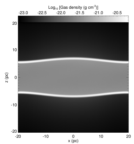
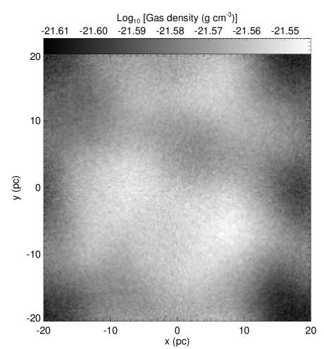
Figure 11: (a) Slice in the $x$-$z$ plane through the density field in $256^{3}$ zone run MS256-RT at a time $t=17.4\>{\rm Myr}$. The slice is centered on the midpoint of the simulation volume. (b) As (a), but for a slice in the $x$-$y$ plane. Note the change in density scale compared to figure (a).

Figure 12: Slice in the $x$-$z$ plane through the density field in $256^{3}$ zone run MS256-RT at a time $t=20.6\>{\rm Myr}$. The slice is centered on the midpoint of the simulation volume.

The morphology of the gas in run MS256 at an output time shortly before the Truelove criterion is violated is also sheet-like, as we can see from Figure 13. However, the width of the sheet in run MS256 is much smaller, and the density cross-section is rather different, with the maximum density being found at the midplane, rather than at the top and bottom edges. As we have already discussed, these differences stem from the differing dynamics of the flow: in this run, photoelectric heating by the ultraviolet background is initially uniform, and so there is no large scale temperature or pressure gradient. The fact that in both runs gravitational collapse produces a sheet-like structure is a consequence of the presence of the magnetic field, which strongly suppresses gas flow perpendicular to the field, but which does not affect flow in the $z$ direction, parallel to the field.

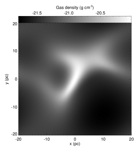
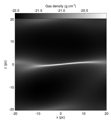
Figure 13: (a) Slice in the $x$-$y$ plane through the density field in $256^{3}$ zone run MS256 at a time $t=28.5\>{\rm Myr}$. The periodic boundary conditions employed in the simulation have allowed us to shift the image so that the densest region lies at the centre of the figure. (b) As (a), but for a slice in the $x$-$z$ plane.

The spatial distribution of $\rm{H}_{2}$ in these simulations is also of interest. In Figure 14 we show how the $\rm{H}_{2}$ fraction varies with position in run MS256-RT. Figure 15 gives the corresponding results for run MS256. In both runs, there is an obvious correlation between the gas density and the $\rm{H}_{2}$ fraction, with the largest molecular fractions being found in the densest gas. However, this correlation is much stronger in run MS256 than in run MS256-RT, because in the former run, the amount of shielding is purely a function of the local gas density, so $\rm{H}_{2}$ both forms faster and is photodissociated more slowly in denser gas. In run MS256-RT, the correlation between local gas density and photodissociation rate is much weaker (although not completely absent).

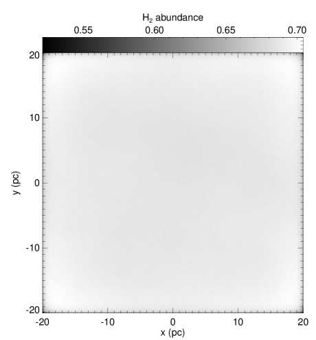
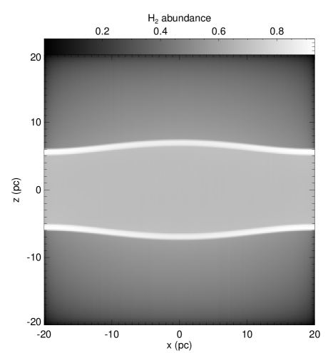
Figure 14: (a) Slice in the $x$-$y$ plane through $256^{3}$ zone run MS256-RT at time $t=17.4\>{\rm Myr}$ showing the spatial variation of the $\rm{H}_{2}$ fraction. The slice is centered on the midpoint of the simulation volume. (b) As (a), but for a slice in the $x$-$z$ plane.

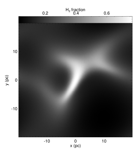
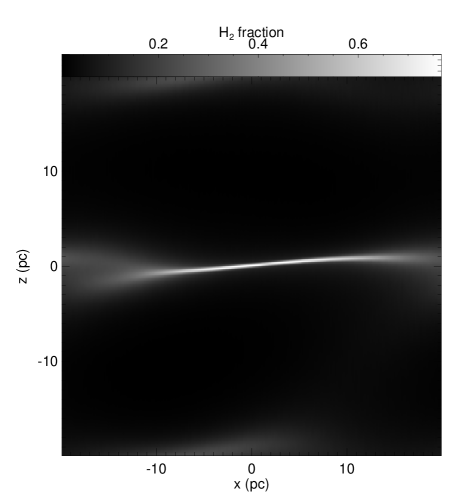
Figure 15: (a) Slice in the $x$-$y$ plane through $256^{3}$ zone run MS256 at time $t=28.5\>{\rm Myr}$ showing the spatial variation of the $\rm{H}_{2}$ fraction. The peak value in this slice is 0.77. (b) As (a), but for a slice in the $x$-$z$ plane.

To better quantify the relationship between gas density and $\rm{H}_{2}$ fraction, we examined how the mean $\rm{H}_{2}$ fraction varied as a function of $n$ in each simulation. To do this, we computed $x_{\rm{H}_{2}}$ and $n$ for each grid zone, and then binned the data by number density, using bins of width 0.05 dex. We then computed the mean and standard deviation for $x_{\rm{H}_{2}}$ for each bin. The resulting values are plotted is Figure 16a for run MS256-RT and Figure 16b for run MS256. Although the mean values that we compute here are volume weighted, we would not expect the mass weighted values to differ greatly, since the narrow width of our density bins means that there is little variation in the gas mass from zone to zone within a given bin.

Figure 16: (a) $\rm{H}_{2}$ fraction as a function of the number density of the gas (crosses) for $256^{3}$ zone run MS256-RT at time $t=17.4\>{\rm Myr}$. To compute these values, we binned the data by number density, using bins of width 0.05 dex, and computed the mean value of $x_{\rm{H}_{2}}$ for each bin. The standard deviation in the value of $x_{\rm{H}_{2}}$ in each bin is also indicated (where it exceeds the size of the symbol). (b) As (a), but for run MS256 at time $t=28.5\>{\rm Myr}$. In this figure, we also indicate the mean value of $x_{\rm H_{2},eq}$ in each bin (dotted line).

An immediately obvious feature of Figure 16a is the discontinuity at $n=100\>{\rm cm^{-3}}$. This feature is a result of the fact that some of the $\rm{H}_{2}$ that forms in the overdense regions bounding the collapsing slab is left behind by the collapse, and so finds itself ultimately in a region with $n<100\>{\rm cm^{-3}}$. In other words, most of the gas at $n<100\>{\rm cm^{-3}}$ did not form in situ, but instead formed at higher densities and has been transported to lower densities. On the other hand, gas with $n>100\>{\rm cm^{-3}}$ resides in the dense slab, and much of this gas has yet to be greatly affected by the collapse (as is apparent from Figure 14).

We do not see a comparable feature in Figure 16b. This is not unexpected, as the dynamics of the flow are quite different in this case, with collapse happening far more slowly. Moreover, the local shielding approximation used in run MS256 leads naturally to a tight relationship between density and $\rm{H}_{2}$ fraction at low densities, as the gas is close to photodissociation equilibrium. This can be seen clearly in Figure 16b if one compare the simulation results with the curve indicating how $x_{\rm H_{2},eq}$ varies with density. The latter curve was constructed by first computing $x_{\rm H_{2},eq}$ for each grid zone (assuming shielding to be described by our local shielding approximation) and then binning and averaging these values using the same procedure as for $x_{\rm{H}_{2}}$. Note that in run MS256-RT we expect $x_{\rm H_{2},eq}$ to vary with both density and with position within the simulation volume, and so we have not constructed a similar curve for this run.

It is also of interest to ask how the $\rm{H}_{2}$ mass is distributed as a function of density. The plots given above show how the $\rm{H}_{2}$ fraction varies with density, but contain no information on how much gas is to be found at any given density. This information is given by the mass-weighted density probability distribution function (PDF), which we have plotted for runs MS256-RT and MS256 in Figures 17a and 17b respectively.

Figure 17: (a) Mass-weighted density PDF, $p_{m}(n)$, in $256^{3}$ zone run MS256-RT at times $t=17.4\>{\rm Myr}$ (solid line) and $t=20.6\>{\rm Myr}$ (dotted line). Note that gas at $n>5500\>{\rm cm^{-3}}$ is not properly resolved by the code, and so the gas distribution at $t=20.6\>{\rm Myr}$ may not be quantitatively accurate (although it should be qualitatively correct). (b) As (a), but for run MS256 at output times $t=28.5\>{\rm Myr}$ (solid line) and $t=31.7\>{\rm Myr}$ (dotted line).

Figure 17 demonstrates that in both runs, much of the gas remains close to the initial density. In run MS256-RT there is also a substantial amount of gas at $n>1000\>{\rm cm^{-3}}$, corresponding to gas associated with the overdensities bounding the collapsing slab. In run MS256, this feature is absent, but there is nevertheless a high density tail, extending up to $n\simeq 4000\>{\rm cm^{-3}}$. In run MS256-RT, about 30% of the total $\rm{H}_{2}$ mass is associated with the relatively unperturbed gas within the slab, with the other 70% being associated with the overdense, collapsing gas (see Figure 18). On the other hand, in run MS256, most of the $\rm{H}_{2}$ is located at densities close to the initial gas density; indeed, only half of the total amount of $\rm{H}_{2}$ is found at $n>100\>{\rm cm^{-3}}$.

Figure 18: (a) Cumulative mass distribution of $\rm{H}_{2}$ with $n$ in $256^{3}$ zone run MS256-RT at times $t=17.4\>{\rm Myr}$ (solid line) and $t=20.6\>{\rm Myr}$ (dotted line). (b) As (a), but for run MS256 at output times $t=28.5\>{\rm Myr}$ (solid line) and $t=31.7\>{\rm Myr}$ (dotted line).

However, as the gas continues to gravitationally collapse, we expect both the PDF and the cumulative mass distribution of $\rm{H}_{2}$ to alter greatly, as we know already that most of the mass and most of the $\rm{H}_{2}$ will ultimately be located in dense, unresolved gas. This is borne out by the results from the end of the simulations which are also plotted in Figures 17 and 18 for runs MS256-RT and MS256.

5.4 Gas temperature: evolution and distribution

As we have previously noted, the cooling time of the gas in our simulations is much shorter than the dynamical timescale. Therefore, the gas very quickly cools to the thermal equilibrium temperature (which for a gas density of $100\>{\rm cm^{-3}}$ is approximately $65\>{\rm K}$, if we use our local shielding approximation) regardless of the initial temperature of the cloud. This is clearly illustrated in Figure 19, where we plot the evolution with time of the minimum and maximum gas temperatures $T_{\rm min}$ and $T_{\rm max}$ in run MS256 (which has an initial gas temperature $T_{\rm i}=1000\>{\rm K}$) and run MS256-T100 (which has $T_{\rm i}=100{\rm K}$ but is otherwise identical to run MS256). Following an initial period of cooling that lasts for approximately $0.05\>{\rm Myr}$, the behaviour of the two runs becomes essentially identical. We see a similarly rapid initial phase of cooling in runs performed using the six-ray shielding approximation.

Figure 19: (a) Evolution with time of the minimum and maximum gas temperatures, $T_{\rm min}$ and $T_{\rm max}$, in $256^{3}$ zone runs MS256 (solid lines) and MS256-T100 (dashed lines), which were performed with initial temperatures of 1000 K and 100 K respectively. (b) Evolution with time of $T_{\rm min}$ and $T_{\rm max}$ in $256^{3}$ zone run MS256-RT.

In run MS256, the temperature distribution following the initial cooling phase is almost uniform, and remains so until the runaway gravitational collapse of the gas begins at $t\sim 20\>{\rm Myr}$. On the other hand, in run MS256-RT we see that even at early times there is a temperature difference of approximately 20 K between $T_{\rm min}$ and $T_{\rm max}$. This temperature differential is a result of the fact that gas at the center of the box is more shielded from photoelectric heating than gas at the edge, and, as we have already discussed, this gives rise to a pressure gradient that drives the subsequent gas flow.

In both runs, we find tight correlations between the gas density and the temperature, as we demonstrate in Figure 20. In run MS256-RT, we see that there is a discontinuity at $n=100\>{\rm cm^{-3}}$. Gas at densities $n>100\>{\rm cm^{-3}}$ is located within the collapsing slab, and so is shielded from the ultraviolet background by the gas in the overdense regions that bound the slab. On the other hand, gas at $n<100{\rm cm^{-3}}$ is located either above or below the slab and so only receives the benefit of this shielding in one direction. Since the contribution from the lightly shielded direction dominates, the result is that the photoelectric heating rate is considerably higher in this gas than in the dense gas in the slab, and so consequently $T_{\rm eq}$ is also higher. No comparable effect is seen in run MS256, as this is a consequence of the non-local nature of the dust shielding and so is not captured by the local shielding approximation.

Figure 20: (a) Mean gas temperature $T$ plotted as a function of the number density $n$ in $256^{3}$ zone run MS256-RT at time $t=17.4\>{\rm Myr}$. The data were binned as in Figure 16 above. The standard deviation in each bin is also indicated whenever it is larger than the size of the symbols used in the plot. (b) As (a), but for run MS256 at time $t=28.5\>{\rm Myr}$.

We have also examined whether one can usefully describe the behaviour of gas in these simulations using a polytropic equation of state. In other words, if we write the gas pressure as a polynomial function of density:

$$p=K\rho^{\gamma_{\rm eff}},$$ (61)

then what functional form must $\gamma_{\rm eff}$ have if this relation is to accurately describe the gas? If $\gamma_{\rm eff}$ is a constant, independent of the density, then the gas is a simple polytrope. Even if $\gamma_{\rm eff}$ is not constant, however, this description can be useful provided that $\gamma_{\rm eff}$ varies smoothly and simply with $\rho$.

Figure 21: (a) Value of $\gamma_{\rm eff}$ as a function of $n$ in $256^{3}$ zone run MS256-RT at time $t=17.4\>{\rm Myr}$. The data were binned as indicated in the text. (b) As (a), but for run MS256 at time $t=28.5\>{\rm Myr}$. Note the difference in the vertical scale compared to Figure 21a.

To investigate how $\gamma_{\rm eff}$ varies as a function of density at late times in each run, we computed the thermal pressure $p$ for each grid zone and then binned the data with density just as we did for the temperature above. We then used the resulting curve, together with the fact that

$$\gamma_{\rm eff}=\frac{{\rm d}\ln p}{{\rm d}\ln\rho}$$ (62)

to compute $\gamma_{\rm eff}$ as a function of density. The values we obtained for runs MS256-RT and MS256 are plotted in Figures 21a and 21b respectively.

Figure 21a demonstrates clearly that the gas in run MS256-RT is not well described by a polytropic equation of state. The prominent feature at $n\sim 100\>{\rm cm^{-3}}$ is a consequence of the discontinuity in the temperature curve at this density and should perhaps be disregarded (since one might still hope to use a polytropic description for the gas within and without the slab, even if the polytropic index for one differs from that for the other). However, from the figure it is clear that even at densities $n\gg 100\>{\rm cm^{-3}}$ and $n\ll 100\>{\rm cm^{-3}}$ a polytropic equation of state is not really appropriate, as there is considerable variation in $\gamma_{\rm eff}$ with $n$. Nevertheless, it is clear that the equation of state of the gas is softer than isothermal, considerably so at low densities.

In run MS256, the polytropic approximation fares much better. Although the gas is not a polytrope, since $\gamma_{\rm eff}$ varies with density, the rate of change of $\gamma_{\rm eff}$ is typically small. For the range of gas densities covered by our simulations, $\gamma_{\rm eff}\sim 0.7$–$0.8$, and so for many applications, treating the gas as a simple polytrope with a constant polytropic exponent that is within this range of values may be a reasonable approximation. We hypothesize that the polytropic description does much better in this case because when we use the local shielding approximation, all of the heating and cooling terms in the energy equation become smooth functions of density. This is not the case in the six-ray runs, as the non-local shielding disrupts the simple relationship between density and photoelectric heating rate.

It is also interesting to examine how the values of $\gamma_{\rm eff}$ derived here compare with previous suggestions in the literature. Our values are significantly smaller than those derived by Spaans & Silk (2000) from their numerical models of solar metallicity gas with this range of densities. However, the values found in run MS256 are only slightly smaller than the value of $\gamma_{\rm eff}=0.725$ derived by Jappsen et al. (2005) from a synthesis of a variety of observational and theoretical sources. In run MS256-RT, the value of $\gamma_{\rm eff}$ at low densities is considerably smaller still, but at higher densities there is better agreement. Nevertheless, it is important to bear in mind that our treatment of the gas chemistry remains highly approximate, and that this, plus the crude nature of our shielding approximations, will limit the accuracy with which we can model the gas temperature. It is therefore unclear how seriously we should take the differences between our results and those of Spaans & Silk (2000) or Jappsen et al. (2005). It would be interesting to revisit this point in the future with simulations that include far more of the relevant carbon and oxygen chemistry and a better treatment of the photoelectric heating.

Finally, we have investigated how the current uncertainty in the value of the cosmic ray ionization rate, discussed previously in § 2.2, affects the temperature evolution of the gas in our simulations. To do this, we performed a run, designated MS256-CR, with the same input parameters as run MS256, but taking a large value of $\zeta=10^{-15}\>{\rm s^{-1}}$ for the cosmic ray ionization rate. This value lies at the high end of current determinations (see e.g. McCall et al., 2003) and so this run and run MS256 should bracket the true behaviour. We compare the evolution of $T_{\rm min}$ and $T_{\rm max}$ in these two runs in Figure 22. We see from the figure that prior to the onset of runaway gravitational collapse, the effect of the higher cosmic ray ionization rate is to increase both $T_{\rm min}$ and $T_{\rm max}$ by about 20 K. However, once collapse begins, the difference between the runs is quickly erased.

The higher temperatures resulting from the higher ionization rate have some influence on the $\rm{H}_{2}$ formation rate. At early times, the net effect is small: the higher gas temperature leads to a slightly higher rate coefficient for $\rm{H}_{2}$ formation, and so to a higher $\rm{H}_{2}$ abundance, but the difference is at the level of about 10%. At late times, once gravitational collapse is well underway, the numbers reported in Table 5 suggest a rather more substantial difference between the runs. However, most of this difference is illusory, and is a consequence of the fact that the higher temperature of the gas in run MS256-CR is matched by a higher Jeans mass, allowing us to resolve the collapse for about 0.5 Myr longer. We therefore resolve more of the $\rm{H}_{2}$ formation that occurs during this run.

We also briefly investigated the effects of using a higher value of $\zeta$ in combination with our six-ray approximation. However, low resolution test runs suggested that the differences were no larger than the differences between runs MS256 and MS256-CR, so we did not pursue this line of investigation further.

Figure 22: Evolution with time of the minimum and maximum gas temperatures, $T_{\rm min}$ and $T_{\rm max}$, in $256^{3}$ zone runs MS256 (solid lines) and MS256-CR (dashed lines), which were performed with cosmic ray ionization rates $\zeta=10^{-17}\>{\rm s^{-1}}$ and $\zeta=10^{-15}\>{\rm s^{-1}}$ respectively.

5.5 Sensitivity to variations of the input parameters

Having explored in some detail the formation and distribution of $\rm{H}_{2}$ in our standard runs, and the thermal behaviour of the gas, it is now time to turn our attention to examining what happens when our input parameters are varied from their standard values. Therefore, in § 5.5.1–5.5.4 below, we examine the effects of varying the box size $L$, the initial perturbation amplitude $\delta$, the initial magnetic field strength $B_{\rm i}$ and the initial density $n_{\rm i}$, while holding the other parameters constant.

5.5.1 Box size

By varying the size of the box while keeping the density of gas within it fixed, we can alter the number of Jeans masses of gas which the box contains and so make the gas either more stable against gravitational collapse (if we decrease $L$) or less stable against collapse (if we increase $L$). If the results of our fiducial simulations are to be considered to be properly representative of the behaviour of real gas, then we should ensure that they are insensitive to small changes in $L$. We therefore performed several additional simulations with our standard set of input parameters, but using different values for $L$. Specifically, we performed four additional $256^{3}$ runs using the local shielding approximation, with $L=20$, 30, 50 and $60\>{\rm pc}$ respectively, and two additional runs using the six-ray approximation, with $L=20$ and $60\>{\rm pc}$ respectively. The results of these runs are plotted in Figure 23, along with the results from runs MS256 and MS256-RT for comparison.

Figure 23: (a) Evolution of $\langle x_{\rm{H}_{2}}\rangle_{\rm M}$ with time in a set of $256^{3}$ zone runs in which $L$ was varied from 20 pc to 60 pc. The three lines in the upper left represent runs MS256-RT-L20 (solid line), MS256-RT (dashed line) and MS256-RT-L60 (dot-dashed line). The five lines in the bottom right represent runs MS256-L20 (lower solid line), MS256-L30 (dashed line), MS256 (dot-dashed line), MS256-L50 (dotted line) and MS256-L60 (upper solid line). (b) As (a), but for the maximum gas density, $\rho_{\rm max}$.

We see that in the runs using the local shielding approximation, increasing $L$ at fixed numerical resolution increases the value of $\langle x_{\rm{H}_{2}}\rangle_{\rm M}$ at all times. This is easy to understand as in these runs, the amount of shielding is proportional to the grid zone size $\Delta x$, and if we increase $L$ while keeping the numerical resolution fixed, then we increase $\Delta x$. It is also apparent that in these runs the rapid increase in $\langle x_{\rm{H}_{2}}\rangle_{\rm M}$ that is caused by the runaway collapse of the gas occurs earlier in runs with a larger value of $L$. Figure 23b demonstrates that this is because runaway gravitational collapse occurs at progressively earlier times as $L$ is increased and at later times as $L$ is decreased. This is a straightforward consequence of the presence of an increased number of Jeans masses in the larger simulations compared to the smaller ones. However, it should be noted that the changes to $L$ change the collapse time of the gas by no more than 20%. Therefore, while magnetic and thermal pressure are clearly playing some role in retarding the collapse of the gas in our fiducial simulations, the effect is not so large as to render the results of these runs unrepresentative of the general case, particularly given the level of approximation to which we are working.

In the runs using the six-ray approximation, we see much less sensitivity to the box size, which again is not unexpected, given that the shielding in these runs is not directly dependent on $\Delta x$. The main effect that is apparent is that $\rm{H}_{2}$ forms slightly more efficiently at early times and considerably more efficiently at late times in runs with a smaller $L$. This appears to be a consequence of the pressure-driven dynamics of the flow, which we have already discussed in some detail in previous sections. In runs with a smaller $L$ it takes less time for the overdense gas layers to propagate to the center of the box, and so therefore it also takes less time for the gas to reach a state of runaway gravitational collapse, as can be seen clearly in Figure 23b. The more rapid density evolution in runs with smaller $L$ leads to a more rapid growth of $\rm{H}_{2}$. Nevertheless, the difference between the runs remains relatively small, suggesting again that our fiducial simulation is adequately representative of the general case.

5.5.2 Initial perturbation amplitude

Since we use periodic boundary conditions in our simulations, a perfectly uniform distribution of gas will be in dynamical equilibrium (albeit an unstable equilibrium on scales larger than the Jeans length) and so will not collapse. To provoke collapse, it is necessary to perturb the distribution. In our simulations of turbulent gas, described in paper II, large perturbations are rapidly created by the motion of the gas. Similarly, in the runs described here which used the six-ray shielding approximation, the pressure gradient caused by the non-uniform photoelectric heating drives a flow that creates density perturbations large enough to trigger gravitational collapse. However, in the runs we performed that used the local shielding approximation, it was necessary to add some form of initial perturbation by hand. Our technique for doing so has already been described, but it is important to understand to what extent our results depend on our choice of $\delta$, the maximum amplitude of the initial random perturbations. Specifically, we would like to know whether the long delay before runaway gravitational collapse begins in earnest in our simulations is a consequence of our choice of a small value for $\delta$. Therefore, we have run several simulations in which we have varied $\delta$ while keeping the other parameters fixed at their fiducial values.

The growth of $\langle x_{\rm{H}_{2}}\rangle_{\rm M}$ with time in $256^{3}$ zone runs with $\delta=0.1$, 0.5 and 1.00, as well as in run MS256 is shown in Figure 24. Clearly, increasing $\delta$ does decrease the time that elapses before runaway collapse occurs, as can also be seen from the results summarized in Table 5. Nevertheless, the time required to form significant quantities of $\rm{H}_{2}$ remains long even in the $\delta=1.00$ case, and while we could reduce the timescale even further by considering even larger inhomogeneities, at this point we would essentially be considering a collection of smaller, denser clouds, rather than a single cloud with a well-defined initial density. Therefore, although the timescale for collapse in these runs does depend on the initial density structure of our cloud, we can nevertheless be certain that it is of the order of 20 Myr or more for an approximately uniform cloud initially at rest.

We also investigated the sensitivity of runs that use our six-ray approximation to variations in $\delta$, since these runs are also seeded with small perturbations to the initially uniform density. As expected, these runs show essentially no sensitivity to $\delta$: the aforementioned pressure-driven effects dominate.

Figure 24: Evolution of $\langle x_{\rm{H}_{2}}\rangle_{\rm M}$ with time in a set of $256^{3}$ zone runs in which the maximum amplitude of the initial density perturbations, $\delta$, was varied. Results are plotted for runs MS256-RT and MS256-RT-d100 (solid and dashed lines in the upper left) as well as for runs MS256 (solid line), MS256-d10 (dashed line), MS256-d50 (dot-dashed line) and MS256-d100 (dotted line). The first pair of runs have $\delta=0.05$ and 1.0 respectively; the latter four have $\delta=0.05$, 0.1, 0.5 and 1.0 respectively.

5.5.3 Initial magnetic field strength

In order to explore how our results depend on the strength of the initial magnetic field, we performed several sets of runs in which we varied the strength of the field but kept all of the other input parameters the same as in our fiducial runs. Specifically, we performed two additional runs using the six-ray shielding approximation: one with an initial field strength $B_{\rm i,fid}=23.4\>\mu{\rm G}$, corresponding to a mass-to-flux ratio of two, in units of the critical value, and one with a field strength of zero, i.e. a purely hydrodynamical run. The evolution with time of $\langle x_{\rm{H}_{2}}\rangle_{\rm M}$ in these runs is plotted in Figure 25a, along with the corresponding values from run MS256-RT. We see that at $t>14\>{\rm Myr}$, the $\rm{H}_{2}$ fraction rises more rapidly in our hydrodynamical run than in our MHD runs, and also that the behaviour of the latter runs is essentially indistinguishable. Figure 25b, which shows the evolution with time of $\rho_{\rm max}$ in these three runs, demonstrates that difference in behaviour between the run with $B=0$ and the runs with $B\neq 0$ is caused by the fact that gravitational collapse occurs more rapidly in the former run than in the latter runs. This is a simple consequence of the fact that in the absence of the magnetic field, gas can flow freely in every direction, allowing the cloud to collapse along all three of its axes at once, while when a magnetic field is present, the gas flow is channeled primarily along the field lines, leading to collapse along only one axis. This also explains why our results are not particularly sensitive to the strength of the field, when one is present, as this will have no effect on the velocity of the flow parallel to the field lines.

Figure 25: (a) Evolution of $\langle x_{\rm{H}_{2}}\rangle_{\rm M}$ with time in a set of $256^{3}$ zone runs in which the strength of the initial magnetic field was varied. Results are plotted for seven runs. Three of these runs used the six-ray shielding approximation: runs HS256-RT (upper solid line), MS256-RT (upper dashed line) and MS256-RT-Bx4 (upper dot-dashed line), which had initial magnetic field strengths $B_{\rm i}=0.0$, 5.85 and $23.4\>\mu{\rm G}$ respectively. The other four runs used the local shielding approximation: runs HS256 (lower solid line), MS256 (lower dashed line), MS256-Bx2 (lower dot-dashed line) and MS256-Bx4 (lower dotted line), which had initial magnetic field strengths $B_{\rm i}=0.0$, 5.85, 11.7 and $23.4\>\mu{\rm G}$ respectively. In the magnetized runs, there is so little sensitivity to $B_{\rm i}$ that the lines are hard to distinguish from each other in the plot. On the other hand, in the $B_{\rm i}=0$ runs we see a significant difference in behaviour. (b) As (a), but for the maximum gas density $\rho_{\rm max}$.

We also examined the sensitivity of the results from the local shielding approximation simulations to the value of $B_{\rm i}$, using values of 0.0, $11.7\>\mu{\rm G}$ and $23.4\>\mu{\rm G}$, and found very similar results: collapse occurs faster and $\rm{H}_{2}$ forms more quickly in the complete absence of a magnetic field, but if a field is present then the timescales for either are not very sensitive to its strength.

5.5.4 Initial density

A final interesting topic to examine is the sensitivity of our results to the initial density of the gas. For instance, if we reduce the initial number density $n_{\rm i}$ from its fiducial value of $100\>{\rm cm^{-3}}$, which is on the high side for the CNM, to $30\>{\rm cm^{-3}}$ or $10\>{\rm cm^{-3}}$, what effect will this have on the timescale for $\rm{H}_{2}$ formation? Obviously, if we reduced $n_{\rm i}$ but kept $L$ constant, then we would reduce the amount of gas in our simulation volume and thereby alter how well the gas could resist gravitational collapse, just as we did when we reduced $L$ while keeping $n_{\rm i}$ constant. Therefore, to examine the effect of changing the density without significantly affecting the gravitational stability of the gas, we must increase $L$ at the same time that we decrease $n_{\rm i}$. Similarly, if we decrease $n_{\rm i}$ and increase $L$, we must also alter $B_{\rm i}$ if we wish to keep the mass-to-flux ratio constant, and hence ensure that the field cannot completely prevent the gas from collapsing.

We therefore performed three simulations with lower initial densities than in our fiducial simulations. In run MS256-RT-n10, we set $n_{\rm i}=10\>{\rm cm^{-3}}$ and used our six-ray shielding approximation. In runs MS256-n10 and MS256-n30, we set $n_{\rm i}=10$ and $30\>{\rm cm^{-3}}$ respectively, and used our local shielding approximation. In all three cases, the box size and magnetic field strength were adjusted so as to keep the number of Jeans masses in the simulation volume and the mass-to-flux ratio approximately the same as in our fiducial runs (see Table 4 for the values used). The evolution of $\langle x_{\rm{H}_{2}}\rangle_{\rm M}$ in these simulations, as well as in runs MS256 and MS256-RT for comparison, is plotted in Figure 26a. In Figure 26b, we show a similar plot for $\rho_{\rm max}$

Figure 26: (a) Evolution of $\langle x_{\rm{H}_{2}}\rangle_{\rm M}$ with time in a set of $256^{3}$ runs in which the initial gas density was varied. Results are plotted for runs MS256-RT (lefthand solid line), MS256-RT-n10 (lefthand dashed line), MS256 (righthand solid line), MS256-n30 (righthand dashed line) and MS256-n10 (dot-dashed line). Note that $L$ and $B_{\rm i}$ were varied in these runs so as to keep the number of Jeans masses in the simulation volume and the mass-to-flux ratio approximately constant. (b) As (a), but for $\rho_{\rm max}$.

Comparison of the evolution of $\langle x_{\rm{H}_{2}}\rangle_{\rm M}$ in the various runs (see Figure 26a) demonstrates that the reduction in $n_{\rm i}$ has a huge effect on the evolution of $\langle x_{\rm{H}_{2}}\rangle_{\rm M}$ at early times in runs performed using the local shielding approximation. This is a consequence of the dramatic reduction in $x_{\rm H_{2},eq}$ in these runs, which decreases from $\sim 0.1$ in run MS256 to $\sim 4\times 10^{-5}$ in run MS256-n30 and to $\sim 7\times 10^{-6}$ in run MS256-n10. Substantial quantities of $\rm{H}_{2}$ are produced in run MS256-n30 only once the gravitational collapse of the gas is well underway and the density in the collapsing gas has become high enough to allow for effective self-shielding on small scales. Since the reduction in $n_{\rm i}$ from $100\>{\rm cm^{-3}}$ to $30\>{\rm cm^{-3}}$ more than doubles the time required for the gas to collapse, this means that we do not see significant $\rm{H}_{2}$ formation before $t\sim 40\>{\rm Myr}$. In run MS256-n10, substantial quantities of $\rm{H}_{2}$ are never produced, even after 100 Myr (although we suspect that if we were to run the simulation for considerably longer, we would see significant $\rm{H}_{2}$ formation, as the gas in this run has only just begun to collapse at the point when the simulation is ended).

In run MS256-RT-n10, the effect of the reduced density is less pronounced, but is significant nonetheless. The reduction of $n_{\rm i}$ by an order of magnitude leads to a reduction in $\langle x_{\rm{H}_{2}}\rangle_{\rm M}$ by roughly a factor of seven at early times. The reduction in $n_{\rm i}$ again leads to an increase in the time required for gravitational collapse to occur, and the gas in run MT256-RT-n10 does not become dominated by $\rm{H}_{2}$ until collapse occurs at $t\sim 50\>{\rm Myr}$.

In practice, of course, we do not expect the gravitational collapse of gas clouds with mean densities of 10 or $30\>{\rm cm^{-3}}$ to take quite as long as these simulations suggest, as the use of periodic boundary conditions to treat real clouds with these densities, and with the sizes considered here, is unlikely to be a good approximation – there is simply too much inhomogeneity in the ISM on these scales. Nevertheless, even if we were to disable the periodic boundary conditions and to treat the gas as an isolated cloud in free-fall collapse (i.e. if we could ignore its thermal and magnetic energy content), then we would still expect gravitational collapse, together with the associated $\rm{H}_{2}$ formation, to occur on a timescale of the order of 10 Myr or more. We show in paper II that the results of turbulent simulations with the same mean density are dramatically different.

6 Summary

In this paper, we have discussed in detail how we have modified the ZEUS-MP hydrodynamical code to allow us to simulate the formation and destruction of $\rm{H}_{2}$ in the ISM. We have used two different approaches for modeling the shielding of $\rm{H}_{2}$ against photodissociation. The first of these is a local shielding approximation, novel to this work, which is computationally efficient and which has the advantage of being biased in a known way: it will always underestimate the amount of shielding, and so we will overestimate the photodissociation rate of $\rm{H}_{2}$. The second approach that we have used is our so-called six-ray approximation, in which we compute $\rm{H}_{2}$ and dust column densities only along the three coordinate axes of the simulation volume. This approach is similar to one used previously by Nelson & Langer (1997, 1999) and by Yoshida et al. (2003), but we believe that this is the first time that it has been applied in grid-based simulations of this scale. This approximation does a much better job of capturing the shielding due to dust, but will tend to overestimate the amount of $\rm{H}_{2}$ self-shielding once the flow velocities become supersonic. For the simulations presented in this paper, it proves to be the better choice, but for the simulations of turbulent gas presented in paper II, the local shielding approximation proves to be more useful.

Our modifications to ZEUS-MP also include a detailed treatment of the thermal behaviour of the gas. By computing the effects of the most important heating and cooling processes active in the ISM, we are able to follow the thermal evolution of the gas with far more accuracy than if we relied upon a description in terms of a simple equation of state, whether isothermal or polytropic. In dense gas, our accuracy is limited by our inability to fully resolve the cooling length of the gas, with the result that we will tend to overproduce warm gas. However, the impact of this on the simulations presented in this paper appears to be small.

In § 3, we discussed how the modified code was tested, and presented the results of a test designed to reproduce the Wolfire et al. (2003) analysis of the thermal equilibrium state of the neutral atomic ISM. Although we do not reproduce their results exactly – most likely due to the fact that the chemical network used in our simulations is very much simpler than that adopted in their analysis – we do find qualitatively similar behaviour. Moreover, a quantitative comparison of the two sets of results suggests that at most densities, our value for the equilibrium gas temperature is accurate to within 50% or better; only for gas at densities $n\sim 1\>{\rm cm^{-3}}$, which lies in the middle of the thermally unstable regime, do we find larger errors, and even here we are accurate to within a factor of two.

Although our main goal in making these modifications was to study $\rm{H}_{2}$ formation in turbulent gas (with results that we report on in paper II), we also applied our modified hydrodynamical code to the problem of $\rm{H}_{2}$ formation in gravitationally collapsing gas without turbulence, starting from initial conditions in which the gas was smoothly distributed and initially at rest. We showed that with these initial conditions and an assumed mean density $n_{\rm i}=100\>{\rm cm^{-3}}$, gravitational collapse occurs on a timescale $t_{\rm coll}>t_{\rm ff}$. The precise value of $t_{\rm coll}$ depends on our choice of shielding approximation (as this significantly affects the pressure balance of the gas), and is also sensitive to the size of the simulation volume, the strength of the magnetic field, and in some circumstances to the size of the initial density inhomogeneities. Our use of periodic boundary conditions probably artificially stabilizes the gas to some extent, but even if these were not used, we would still expect collapse to take at least one free-fall time (which for our standard initial density $n_{\rm i}$ is approximately $5\>{\rm Myr}$), and in fact probably significantly longer, since the thermal pressure of the gas is never negligible.

In the simulations that we ran that used the local shielding approximation, we found that $\rm{H}_{2}$ formation occurred in two phases. During the first phase, which had a timescale of 5–$10\>{\rm Myr}$, $\langle x_{\rm{H}_{2}}\rangle_{\rm M}$ grew slowly until it reached a small limiting value, set by the fact that the gas had reached photodissociation equilibrium. Owing to our approximate treatment of $\rm{H}_{2}$ shielding, this limiting value was resolution dependent (and was smaller in higher resolution simulations), but even in our lowest resolution, $64^{3}$ zone simulations, it corresponded to no more than about 25% of the gas being molecular. The second, rapid phase of $\rm{H}_{2}$ formation was triggered by the runaway gravitational collapse of the gas, as the increased density boosted the $\rm{H}_{2}$ formation rate while also increasing the amount of shielding against UV photodissociation. By the end of the simulations, between 50 and 100% of the gas had become molecular, with most of the $\rm{H}_{2}$ having being formed during this collapse phase. Therefore, in these simulations, gravitational collapse drives $\rm{H}_{2}$ formation.

In the simulations that we ran that used the six-ray approximation, the situation was somewhat different. In these runs, the amount of shielding in most of the box was considerably higher, and so the gas generally did not reach photodissociation equilibrium until very late times. Therefore, in these runs $\rm{H}_{2}$ formation was reasonably efficient even in the absence of dynamical effects. However, we have seen that in these runs the fact that the gas in the center is shielded more than the gas at the edges leads to the development of a significant temperature gradient and associated pressure gradient. This drives a flow of gas towards the center of the box, and the presence of a dynamically significant magnetic field causes this flow to be oriented in a direction parallel to the magnetic field lines. The resulting pressure-driven compression is ultimately responsible for triggering runaway gravitational collapse. Once this runaway collapse begins, we see a distinct acceleration in the rate of $\rm{H}_{2}$ formation, and so even in these simulations it is true to say that gravitational collapse plays an important role in driving $\rm{H}_{2}$ formation. These results should be compared with the results from simulations of supersonically turbulent gas that we present in paper II. They demonstrate that once a sufficiently high mean density is reached, whether through gravitational instability or other means, the turbulent compressions alone lead to substantial $\rm{H}_{2}$ formation, with gravitational collapse subsequently playing only a minor role.

We have also examined the spatial distribution of the $\rm{H}_{2}$ produced in our simulations. We have shown that by the end of the simulation, most of the $\rm{H}_{2}$ is to be found in dense gas, with at least 50% in gas denser than $5000\>{\rm cm^{-3}}$. Moreover, since the initial distributions of the gas and the magnetic field are nearly uniform, and since the subsequent dynamical evolution proceeds smoothly, the final spatial distribution is highly ordered. Most of the $\rm{H}_{2}$, and, indeed, most of the gas, are found in a thin, dense sheet oriented perpendicularly to the direction of the magnetic field. Visually, this distribution looks quite unlike that of the molecular gas in real molecular clouds, suggesting that more small-scale power is required in either the initial density distribution or velocity distribution (or both) in order to produce realistic-looking clouds.

Finally, we briefly examined the thermal behaviour of gas in our simulations, and showed that, as expected, most of the gas is in thermal equilibrium, owing to the short cooling times at the simulated gas densities. However, the gas is not isothermal, nor is it describable as a simple polytrope: while we can describe the relationship between density and temperature with a function of the form

$$T\propto n^{\gamma-1},$$ (63)

the polytropic exponent $\gamma$ is not constant, but varies with density as shown in Figure 21. In runs performed using the local shielding approximation, $\gamma_{\rm eff}\sim 0.7$–$0.8$ over the range of densities covered by our simulations, but in runs that used the six-ray approximation, we found a much wider range of $\gamma_{\rm eff}$. We conclude that while there may be some applications for which treating the gas as a simple polytrope with a constant polytropic exponent is a reasonable approximation, this approach is probably not valid in the general case.

Obviously, we do not claim that the results of the study presented in this paper are directly applicable to the real ISM: we have investigated a rather simplified dynamical situation, which is missing one of the main physical ingredients present in the real ISM, namely supersonic turbulence. However, we believe that this study is interesting for the light it sheds on the rate at which molecular clouds will form in the absence of turbulence: as we have seen, in this case substantial quantities of $\rm{H}_{2}$ are formed only on timescales $t>t_{\rm ff}$, consistent with a cloud formation timescale of at least 5–$10\>{\rm Myr}$. As we shall see in paper II, the behaviour of supersonically turbulent gas is very different.

Table 1: The set of chemical reactions that make up our model of non-equilibrium hydrogen chemistry.

Reaction	Reference
1. $\rm{H}+\rm{H}+{\rm grain}\rightarrow\rm{H}_{2}+{\rm grain}$	Hollenbach & McKee (1979)
2. $\rm{H}_{2}+\rm{H}\rightarrow 3\rm{H}$	Mac Low & Shull (1986) (low density),
	Lepp & Shull (1983) (high density)
3. $\rm{H}_{2}+\rm{H}_{2}\rightarrow 2\rm{H}+\rm{H}_{2}$	Martin, Keogh & Mandy (1998) (low density),
	Shapiro & Kang (1987) (high density)
4. $\rm{H}_{2}+\gamma\rightarrow 2\rm{H}$	See § 2.2.1
5. $\rm{H}+{\rm c.r.}\rightarrow\rm{H}^{+}+\rm{e}$	See § 2.2
6. $\rm{H}+\rm{e}\rightarrow\rm{H}^{+}+2\rm{e}$	Abel et al. (1997)
7. $\rm{H}^{+}+\rm{e}\rightarrow\rm{H}+\gamma$	Ferland et al. (1992)
8. $\rm{H}^{+}+\rm{e}+{\rm grain}\rightarrow\rm{H}+{\rm grain}$	Weingartner & Draine (2001)

Table 2: Processes included in our thermal model.

Process	References
Cooling:
C ii fine structure lines	Atomic data – Silva & Viegas (2002)
	Collisional rates ($\rm{H}_{2}$) – Flower & Launay (1977)
	Collisional rates ($\rm{H}$, $T<2000\>{\rm K}$) – Hollenbach & McKee (1989)
	Collisional rates ($\rm{H}$, $T>2000\>{\rm K}$) – Keenan et al. (1986)
	Collisional rates (${\rm e^{-}}$) – Wilson & Bell (2002)
O i fine structure lines	Atomic data – Silva & Viegas (2002)
	Collisional rates ($\rm{H}$, $\rm{H}_{2}$) – Flower, priv. comm.
	Collisional rates (${\rm e^{-}}$) – Bell, Berrington & Thomas (1998)
	Collisional rates ($\rm{H}^{+}$) – Pequignot (1990, 1996)
Si ii fine structure lines	Atomic data – Silva & Viegas (2002)
	Collisional rates ($\rm{H}$) – Roueff (1990)
	Collisional rates (${\rm e^{-}}$) – Dufton & Kingston (1991)
$\rm{H}_{2}$ rovibrational lines	Le Bourlot, Pineau des Forêts & Flower (1999)
Gas-grain energy transfer1	Hollenbach & McKee (1989)
Recombination on grains	Wolfire et al. (2003)
Atomic resonance lines	Sutherland & Dopita (1993)
$\rm{H}$ collisional ionization	Abel et al. (1997)
$\rm{H}_{2}$ collisional dissociation	See Table 1
Heating:
Photoelectric effect	Bakes & Tielens (1994); Wolfire et al. (2003)
$\rm{H}_{2}$ photodissociation	Black & Dalgarno (1977)
UV pumping of $\rm{H}_{2}$	Burton, Hollenbach & Tielens (1990)
$\rm{H}_{2}$ formation on dust grains	Hollenbach & McKee (1989)
Cosmic ray ionization	Goldsmith & Langer (1978)

Note. — 1: If $T_{\rm gas}<T_{\rm grain}$, the net flow of energy is from the grains to the gas, leading to heating instead of cooling.

Table 3: The number density at which the Truelove criterion is violated, $n_{\rm max}$, computed for gas in thermal and chemical equilibrium for various different box sizes and numerical resolutions.

Resolution	Box size (pc)	Zone size (pc)	$n_{\rm max}\>\left({\rm cm}^{-3}\right)$
	20	0.31	$2.0\times 10^{3}$
$64^{3}$	40	0.62	$8.0\times 10^{2}$
	60	0.94	$4.9\times 10^{2}$
	20	0.16	$5.4\times 10^{3}$
$128^{3}$	40	0.31	$2.0\times 10^{3}$
	60	0.47	$1.2\times 10^{3}$
	20	0.078	$1.5\times 10^{4}$
$256^{3}$	40	0.16	$5.4\times 10^{3}$
	60	0.23	$3.0\times 10^{3}$
	20	0.039	$5.6\times 10^{4}$
$512^{3}$	40	0.078	$1.5\times 10^{4}$
	60	0.12	$8.2\times 10^{3}$

Table 4: Input parameters used for our runs

Run	$L$ (pc)	$\delta$	$n_{\rm i}$ ($\rm{cm^{-3}}$)	$T_{\rm i}$ (K)	$B_{\rm i}$ ($\mu$G)	Notes
MS64	40	0.05	100	1000	5.85
MS128	40	0.05	100	1000	5.85
MS256	40	0.05	100	1000	5.85
MS64-RT	40	0.05	100	1000	5.85
MS128-RT	40	0.05	100	1000	5.85
MS256-RT	40	0.05	100	1000	5.85
MS64-ng	40	0.05	100	1000	5.85	1
MS128-ng	40	0.05	100	1000	5.85	1
MS256-ng	40	0.05	100	1000	5.85	1
MS256-RT-ng	40	0.05	100	1000	5.85	1
MS64-nr	40	0.05	100	1000	5.85	2
MS128-nr	40	0.05	100	1000	5.85	2
MS256-nr	40	0.05	100	1000	5.85	2
MS256-T100	40	0.05	100	100	5.85
MS256-CR	40	0.05	100	1000	5.85	3
MS256-L20	20	0.05	100	1000	5.85
MS256-RT-L20	20	0.05	100	1000	5.85
MS256-L30	30	0.05	100	1000	5.85
MS256-L50	50	0.05	100	1000	5.85
MS256-L60	60	0.05	100	1000	5.85
MS256-RT-L60	60	0.05	100	1000	5.85
MS256-Bx2	40	0.05	100	1000	11.7
MS256-Bx4	40	0.05	100	1000	23.4
MS256-RT-Bx4	40	0.05	100	1000	23.4
HS256	40	0.05	100	1000	0.0
HS256-RT	40	0.05	100	1000	0.0
MS256-d10	40	0.10	100	1000	5.85
MS256-d50	40	0.50	100	1000	5.85
MS256-d100	40	1.00	100	1000	5.85
MS256-RT-d100	40	1.00	100	1000	5.85
MS256-n10	85	0.05	10	1000	1.24
MS256-RT-n10	85	0.05	10	1000	1.24
MS256-n30	60	0.05	30	1000	2.63

Note. — 1: runs with self-gravity disabled; 2: runs with $\chi=0.0$; 3: run with a higher cosmic ray ionization rate, $\zeta=10^{-15}\>{\rm s^{-1}}$.

Table 5: $t_{\rm res}$, $t_{\rm f}$, and associated values of $\langle x_{\rm{H}_{2}}\rangle_{\rm M}$ for all runs in Table 4.

Run	$t_{\rm res}$ (Myr)	$\langle x_{\rm{H}_{2}}\rangle_{\rm M}(t_{\rm res})$	$t_{\rm f}$ (Myr)	$\langle x_{\rm{H}_{2}}\rangle_{\rm M}(t_{\rm f})$
MS64	21.3	0.30	27.3	0.89
MS128	26.5	0.34	31.1	0.93
MS256	29.5	0.21	31.7	0.50
MS64-RT	15.0	0.65	22.1	0.99
MS128-RT	16.9	0.74	20.9	0.99
MS256-RT	18.4	0.89	20.6	0.99
MS64-ng	—	—	31.7	0.26
MS128-ng	—	—	31.7	0.13
MS256-ng	—	—	31.7	$6.4\times 10^{-2}$
MS256-RT-ng	—	—	19.9	0.73
MS64-nr	18.3	0.70	29.6	0.99
MS128-nr	22.1	0.76	28.9	0.98
MS256-nr	26.6	0.83	31.7	0.96
MS256-T100	28.9	0.23	31.7	0.62
MS256-CR	30.0	0.42	31.7	0.76
MS256-L20	—	—	31.7	$7.4\times 10^{-2}$
MS256-RT-L20	17.2	0.96	20.0	0.99
MS256-L30	31.3	0.42	31.7	0.48
MS256-L50	27.7	0.20	30.8	0.71
MS256-L60	26.7	0.20	29.9	0.70
MS256-RT-L60	17.8	0.76	22.1	0.98
MS256-Bx2	29.8	0.25	31.7	0.50
MS256-Bx4	29.2	0.27	31.7	0.62
MS256-RT-Bx4	18.7	0.92	19.0	0.96
HS256	23.9	0.10	25.2	0.21
HS256-RT	13.1	0.60	18.2	0.97
MS256-d10	27.1	0.22	30.5	0.68
MS256-d50	22.9	0.20	25.8	0.64
MS256-d100	21.0	0.19	23.7	0.59
MS256-RT-d100	17.1	0.80	20.2	0.99
MS256-n10	—	—	95.1	$8.7\times 10^{-6}$
MS256-RT-n10	—	—	53.0	0.91
MS256-n30	58.1	0.26	64.1	0.70

Note. — $t_{\rm res}$ is the time at which the Truelove criterion is first violated during the course of the run; when no value is given, this indicates that the criterion was never violated. $t_{\rm f}$ is the time at which the simulation was stopped.

References

- Abel et al. (1997) Abel, T., Anninos, P., Zhang, Y., & Norman, M. L. 1997, New Astron., 2, 181
- Bakes & Tielens (1994) Bakes, E. L. O., & Tielens, A. G. G. M. 1994, ApJ, 427, 822
- Ballesteros-Paredes, Hartmann & Vázquez-Semadeni (1999) Ballesteros-Paredes, J., Hartmann, L., & Vázquez-Semadeni, E. 1999, ApJ, 527, 285
- Balsara et al. (2004) Balsara, D. S., Kim, J., Mac Low, M.-M., & Mathews, G. J. 2004, ApJ, 617, 339
- Beck (2001) Beck, R. 2001, Space Science Reviews, 99, 243
- Bell, Berrington & Thomas (1998) Bell, K. L., Berrington K. A., & Thomas, M. R. J. 1998, MNRAS, 293, L83
- Bergin et al. (2004) Bergin, E. A., Hartmann, L. W., Raymond, J. C., & Ballesteros-Paredes, J. 2004, ApJ, 612, 921
- Bergin et al. (1999) Bergin, E. A., Plume, R., Williams, J. P., & Myers, P. C. 1999, ApJ, 512, 724
- Bertoldi (1989) Bertoldi, F. 1989, ApJ, 346, 735
- Black & Dalgarno (1977) Black, J. H., & Dalgarno, A. 1977, ApJS, 34, 405
- Blitz et al. (2006) Blitz, L., Fukui, Y., Kawamura, A., Leroy, A., Mizuno, N., & Rosolowsky, E. 2006, to appear in Protostars and Planets V; astro-ph/0602600
- Burton, Hollenbach & Tielens (1990) Burton, M. G., Hollenbach, D. J., & Tielens, A. G. G. M. 1990, ApJ, 365, 620
- Cardelli, Clayton & Mathis (1989) Cardelli, J. A., Clayton, G. C., & Mathis, J. S. 1989, ApJ, 345, 245
- Caselli et al. (1998) Caselli, P., Walmsley, C. M., Terzieva, R., & Herbst, E. 1998 ApJ, 499, 234
- Cazaux & Tielens (2004) Cazaux, S., & Tielens, A. G. G. M. 2004, ApJ, 604, 222
- Colella & Woodward (1984) Colella, P., & Woodward, P. R. 1984, J. Comp. Phys., 54, 174
- Crutcher (1999) Crutcher, R. M. 1999, ApJ, 520, 706
- Crutcher et al. (2004) Crutcher, R. M., Nutter, D. J., Ward-Thompson, D., & Kirk, J. M. 2004, ApJ, 600, 279
- de Avillez (2000) de Avillez, M. A. 2000, MNRAS, 315, 479
- de Avillez & Breitschwerdt (2004) de Avillez, M. A., & Breitschwerdt, D. 2004, A&A, 425, 899
- Draine (1978) Draine, B. T. 1978, ApJS, 36, 595
- Draine & Bertoldi (1996) Draine, B. T., & Bertoldi, F. 1996, ApJ, 468, 269
- Dufton & Kingston (1991) Dufton, P. L., & Kingston, A. E. 1991, MNRAS, 248, 827
- Duley & Williams (1993) Duley, W. W., & Williams, D. A. 1993, MNRAS, 260, 37
- Elmegreen (1990) Elmegreen, B. G. 1990, in ASP Conf. Ser. 12, The evolution of the interstellar medium, ed. L. Blitz, (San Francisco: ASP), 247
- Elmegreen (2000) Elmegreen, B. G. 2000, ApJ, 530, 277
- Falgarone et al. (1998) Falgarone, E., Panis, J.-F., Heithausen, A., Pérault, M., Stutzki, J., Puget, J.-L., & Bensch, F. 1998, A&A, 331, 669
- Falle (2002) Falle, S. A. E. G. 2002, ApJ, 577, L123
- Ferland et al. (1992) Ferland, G. J., Peterson, B. M., Horne, K., Welsh, W. F., & Nahar, S. N. 1992, ApJ, 387, 95
- Fiedler (1997) Fiedler, R. A. 1997, in Proceedings of the 1997 ACM/IEEE conference on Supercomputing, Conference on High Performance Networking and Computing, (New York: ACM Press), 1, http://doi.acm.org/10.1145/509593.509598
- Field (1965) Field, G. B. 1965, ApJ, 142, 531
- Flower & Launay (1977) Flower, D. R., & Launay, J. M. 1977, J. Phys. B, 10, 3673
- Frigo & Johnson (1998) Frigo, M., & Johnson, S. G. 1998, in Proc. 1998 IEEE Intl. Conf. Acoustics Speech and Signal Processing, 3, 1381
- Fukui et al. (1999) Fukui, Y., et al., 1999, PASJ, 51, 745
- Glover (2003) Glover, S. 2003, ApJ, 584, 331
- Glover & Mac Low (2006) Glover, S. C. O., & Mac Low, M.-M. 2006, ApJ, submitted; astro-ph/0605121 (paper II)
- Goldsmith & Langer (1978) Goldsmith, P. F., & Langer, W. D. 1978, ApJ, 222, 881
- Gould & Salpeter (1963) Gould, R. J., & Salpeter, E. E. 1963, ApJ, 138, 393
- Habing (1968) Habing, H. J. 1968, Bull. Astron. Inst. Netherlands, 19, 421
- Hartmann, Ballesteros-Paredes & Bergin (2001) Hartmann, L., Ballesteros-Paredes, J., & Bergin, E. A. 2001, ApJ, 562, 852
- Hawley & Stone (1995) Hawley, J. F., & Stone, J. M. 1995, Comp. Phys. Comm., 89, 127
- Hayes et al. (2006) Hayes, J. C., Norman, M. L., Fiedler, R. A., Bordner, J. O., Li, P. S., Clark, S. E., ud-Doula, A., & Mac Low, M.-M. 2006, ApJS, 165, 188
- Heiles & Crutcher (2005) Heiles, C., & Crutcher, R. 2005, in Lecture Notes in Physics 664, Cosmic magnetic fields, eds. R. Wielebinski & R. Beck, (Berlin: Springer), 137
- Hennebelle & Pérault (1999) Hennebelle, P., & Pérault, M. 1999, A&A, 351, 309
- Hennebelle & Pérault (2000) Hennebelle, P., & Pérault, M. 2000, A&A, 359, 1124
- Hollenbach & McKee (1979) Hollenbach, D., & McKee, C. F. 1979, ApJS, 41, 555
- Hollenbach & McKee (1989) Hollenbach, D., & McKee, C. F. 1989, ApJ, 342, 306
- Hollenbach & Salpeter (1970) Hollenbach, D., & Salpeter, E. E. 1970, J. Chem. Phys., 53, 79
- Hollenbach & Salpeter (1971) Hollenbach, D., & Salpeter, E. E. 1971, ApJ, 163, 155
- Jappsen et al. (2005) Jappsen, A.-K., Klessen, R. S., Larson, R. B., Li, Y., & Mac Low, M.-M. 2005, A&A, 435, 611
- Joung & Mac Low (2006) Joung, M. K.R., & Mac Low, M.-M. 2006, ApJ, submitted; astro-ph/0601005
- Jura (1974) Jura, M. 1974, ApJ, 191, 375
- Katz et al. (1999) Katz, N., Furman, I., Biham, O., Pirronello, V., & Vidali, G. 1999, ApJ, 522, 305
- Keenan et al. (1986) Keenan, F. P., Lennon, D. J., Johnson, C. T., & Kingston, A. E. 1986, MNRAS, 220, 571
- Kennicutt (1989) Kennicutt, R. C. 1989, ApJ, 344, 685
- Kessel-Deynet & Burkert (2003) Kessel-Deynet, O., & Burkert, A. 2003, MNRAS, 338, 545
- Kim, Ostriker & Stone (2002) Kim, W.-T., Ostriker, E. C., & Stone, J. M. 2002, ApJ, 581, 1080
- Korpi et al. (1999) Korpi, M. J., Brandenburg, A., Shukurov, A., Tuominen, I., & Nordlund, Å. 1999, ApJ, 514, L99
- Koyama & Inutsuka (2000) Koyama, H., & Inutsuka, S. 2000, ApJ, 532, 980
- Koyama & Inutsuka (2002) Koyama, H., & Inutsuka, S. 2002, ApJ, 564, L97
- Koyama & Inutsuka (2004) Koyama, H., & Inutsuka, S. 2004, ApJ, 602, L25
- Kravtsov (2003) Kravtsov, A. V. 2003, ApJ, 590, L1
- Kritsuk & Norman (2002a) Kritsuk, A. G., & Norman, M. L. 2002a, ApJ, 569, L127
- Kritsuk & Norman (2002b) Kritsuk, A. G., & Norman, M. L. 2002b, ApJ, 580, 51
- Kritsuk & Norman (2004) Kritsuk, A. G., & Norman, M. L. 2004, ApJ, 601, L55
- Krumholz, Matzner & McKee (2006) Krumholz, M. R., Matzner, C. D., & McKee, C. F. 2006, astro-ph/0608471
- Larson (1985) Larson, R. B. 1985, MNRAS, 214, 379
- Lazarian & Pogosyan (2000) Lazarian, A., & Pogosyan, D. 2000, ApJ, 537, 720
- Le Bourlot, Pineau des Forêts & Flower (1999) Le Bourlot, J., Pineau des Forêts, G., & Flower, D. R. 1999, MNRAS, 305, 802
- Le Petit, Roueff & Herbst (2004) Le Petit, F., Roueff, E., & Herbst, E. 2004, A&A, 417, 993
- Lepp & Shull (1983) Lepp, S., & Shull, J. M. 1983, ApJ, 270, 578
- Le Teuff, Millar & Markwick (2000) Le Teuff, Y. H., Millar, T. J., & Markwick, A. J. 2000, A&AS, 146, 157
- Li, Mac Low & Klessen (2005) Li, Y., Mac Low, M.-M., & Klessen, R. S. 2005, ApJ, 626, 823
- Liszt (2003) Liszt, H. 2003, A&A, 398, 621
- Mac Low (1999) Mac Low, M.-M. 1999, ApJ, 524, 169
- Mac Low & Klessen (2004) Mac Low, M.-M., & Klessen, R. S. 2004, Rev. Mod. Phys., 76, 125
- Mac Low & Shull (1986) Mac Low, M.-M., & Shull, J. M. 1986, ApJ, 302, 585
- Martin, Keogh & Mandy (1998) Martin, P. G., Keogh W. J., & Mandy, M. E. 1998, ApJ, 499, 793
- Martin, Schwarz & Mandy (1996) Martin, P. G., Schwarz, D. H., & Mandy, M. E. 1996, ApJ, 461, 265
- Matzner (2002) Matzner, C. D. 2002, ApJ, 566, 302
- McCall et al. (2003) McCall, B. J., et al. 2003, Nature, 422, 500
- Nakano & Nakamura (1978) Nakano, T., & Nakamura, T. 1978, PASJ, 30, 671
- Nelson & Langer (1997) Nelson, R. P., & Langer, W. D. 1997, ApJ, 482, 796
- Nelson & Langer (1999) Nelson, R. P., & Langer, W. D. 1999, ApJ, 524, 923
- Neufeld & Kaufman (1993) Neufeld, D. A., & Kaufman, M. J. 1993, ApJ, 418, 263
- Neufeld, Lepp & Melnick (1995) Neufeld, D. A., Lepp, S., & Melnick, G. J. 1995, ApJS, 100, 132
- Norman (2000) Norman, M. L. 2000, RevMexAA, 9, 66
- O’Neill, Viti & Williams (2002) O’Neill, P. T., Viti, S., & Williams, D. A. 2002, A&A, 388, 346
- Ossenkopf (1997) Ossenkopf, V. 1997, New Astronomy, 2, 365
- Padoan & Scalo (2005) Padoan, P., & Scalo, J. 2005, ApJ, 624, L97
- Parker (1953) Parker, E. N. 1953, ApJ, 117, 431
- Parker (1966) Parker, E. N. 1966, ApJ, 145, 811
- Pavlovski et al. (2002) Pavlovski, G., Smith, M. D., Mac Low, M.-M., & Rosen, A. 2002, MNRAS, 337, 477
- Pequignot (1990) Pequignot, D. 1990, A&A, 231, 499
- Pequignot (1996) Pequignot, D. 1996, A&A, 313, 1026
- Pringle, Allen & Lubow (2001) Pringle, J. E., Allen, R. J., & Lubow, S. H. 2001, MNRAS, 327, 663
- Roser et al. (2003) Roser, J. E., Swords, S., Vidali, G., Manicò, G., & Pirronello, V. 2003, ApJ, 596, L55
- Roueff (1990) Roueff, E. 1990, A&A, 234, 567
- Sanders, Solomon & Scoville (1984) Sanders, D. B., Solomon, P. M., & Scoville, N. Z. 1984, ApJ, 276, 182
- Sandford, Whitaker & Klein (1982) Sandford, M. T., II, Whitaker, R. W., & Klein, R. I. 1982, ApJ, 260, 183
- Sandford, Whitaker & Klein (1984) Sandford, M. T., II, Whitaker, R. W., & Klein, R. I. 1984, ApJ, 282, 178
- Sembach et al. (2000) Sembach, K. R., Howk, J. C., Ryans, R. S. I., & Keenan, F. P. 2000, ApJ, 528, 310
- Shapiro & Kang (1987) Shapiro, P. R., & Kang, H. 1987, ApJ, 318, 32
- Silva & Viegas (2002) Silva, A. I., & Viegas, S. M. 2002, MNRAS, 329, 135
- Slyz et al. (2005) Slyz, A. D., Devriendt, J. E. G., Bryan, G., & Silk, J. 2005, MNRAS, 356, 737
- Smith & Rosen (2003) Smith, M. D., & Rosen, A. 2003, MNRAS, 339, 133
- Sobolev (1957) Sobolev, V. V. 1957, Sv. Ast., 1, 678
- Sod (1978) Sod, G. A. 1978, J. Comp. Phys., 27, 1
- Spaans & Silk (2000) Spaans, M., & Silk, J. 2000, ApJ, 538, 115
- Stone & Norman (1992a) Stone, J. M., & Norman, M. L. 1992a, ApJS, 80, 753
- Stone & Norman (1992b) Stone, J. M., & Norman, M. L. 1992b, ApJS, 80, 791
- Stone, Ostriker & Gammie (1998) Stone, J. M., Ostriker, E. C., & Gammie, C. F. 1998 ApJ, 508, L99
- Sutherland & Dopita (1993) Sutherland, R. S., & Dopita, M. A. 1993, ApJS, 88, 253
- Suttner et al. (1997) Suttner, G., Smith, M. D., Yorke, H. W., & Zinnecker, H. 1997, A&A, 318, 595
- van der Tak & van Dishoeck (2000) van der Tak, F. F. S., & van Dishoeck, E. F. 2000, A&A, 358, 79
- Truelove et al. (1997) Truelove, J. K., Klein, R. I., McKee, C. F., Holliman, J. H., Howell, L. H., & Greenough, J. A. 1997, ApJ, 489, L179
- Wada (2001) Wada, K. 2001., ApJ, 559, L41
- Weingartner & Draine (2001) Weingartner, J. C., & Draine, B. T. 2001, ApJ, 563, 842
- Wiklind (2004) Wiklind, T. 2004, in Carnegie Observatories Astrophysics Series, Vol. 4: Origin and Evolution of the Elements, eds. A. McWilliam and M. Rauch, (Cambridge: Cambridge Univ. Press.), 354
- Wilson & Bell (2002) Wilson, N. J., & Bell, K. L. 2002, MNRAS, 337, 1027
- Wolfire et al. (1995) Wolfire, M. G., Hollenbach, D., McKee, C. F., Tielens, A. G. G. M., & Bakes, E. L. O. 1995, ApJ, 443, 152
- Wolfire et al. (2003) Wolfire, M. G., McKee, C. F., Hollenbach, D., & Tielens, A. G. G. M. 2003, ApJ, 587, 278
- Yoshida et al. (2003) Yoshida, N., Abel, T., Hernquist, L., & Sugiyama, N. 2003, ApJ, 592, 645