The Kinematic and Plasma Properties of X-ray Knots in Cassiopeia A from the Chandra HETGS

Abstract

We present high-resolution X-ray spectra from the young supernova remnant Cas A using a 70-ks observation taken by the Chandra High Energy Transmission Grating Spectrometer (HETGS). Line emission, dominated by Si and S ions, is used for high-resolution spectral analysis of many bright, narrow regions of Cas A to examine their kinematics and plasma state. These data allow a 3D reconstruction using the unprecedented X-ray kinematic results: we derive unambiguous Doppler shifts for these selected regions, with values ranging between $-2500$ and $+4000$ km s^-1 and the typical velocity error less than 200 km s^-1. Plasma diagnostics of these regions, derived from line ratios of resolved He-like triplet lines and H-like lines of Si, indicate temperatures largely around 1 keV, which we model as O-rich reverse-shocked ejecta. The ionization age also does not vary considerably over these regions of the remnant. The gratings analysis was complemented by the non-dispersed spectra from the same dataset, which provided information on emission measure and elemental abundances for the selected Cas A regions. The derived electron density of X-ray emitting ejecta varies from 20 to 200 cm^-3. The measured abundances of Mg, Si, S and Ca are consistent with O being the dominant element in the Cas A plasma. With a diameter of 5′, Cas A is the largest source observed with the HETGS to date. We, therefore, describe the technique we use and some of the challenges we face in the HETGS data reduction from such an extended, complex object.

1 Introduction

Cassiopeia A (Cas A, G111.7–2.1) is the youngest Galactic supernova remnant (SNR), believed to be a product of a SN explosion in $\sim 1670$ (e.g. Thorstensen et al., 2001; Fesen et al., 2006). The SNR is the brightest object in the radio band, and is very bright in the X-ray band, providing a suitable target for detailed studies across a wide range of wavelengths. Cas A shows a wealth of phenomena important for studying the SN progenitor, its explosion mechanism, the early evolution of SNRs, and their impact on the interstellar medium.

The remnant appears as a bright, clumpy ring of emission with a diameter of around 3′  associated with the SNR ejecta, while the fainter emission from the SNR forward shock forms a filamentary ring with a diameter of 5′. The almost perfectly circular appearance of the SNR is disrupted by the clear extension in the NE region of the SNR, called the jet, and a less obvious one in the SW called the counter-jet (e.g Fesen & Gunderson, 1996; Hwang et al., 2000).

Many of Cas A’s bright knots have been identified as shocked ejecta, still clearly visible due to the young age of the SNR. Observations in the optical band provided the first insights into the kinematics and chemical composition of these ejecta (e.g. Minkowski, 1959; Peimbert & van den Bergh, 1971; Chevalier & Kirshner, 1978). The optical-emitting ejecta have been classified into two main groups: the fast-moving knots (FMKs), moving with speeds from 4000 km s^-1 up to 15,000 km s^-1, and the slow-moving quasi-stationary floculi (QFS), moving with speeds less than 300 km s^-1 (Kamper & van den Bergh, 1976). The emission from FMKs, believed to be ejecta, is H-deficient (from the lack of H$\alpha$ emission) and dominated by forbidden O and S emission (e.g. Fesen et al., 2001). This lack of hydrogen in FMKs suggests that Cas A was a Type Ib supernova produced by the core-collapse of a Wolf-Rayet star (e.g. Woosley et al., 1993). The emission from QFSs is rich in N, which is the reason these knots are believed to originate from the circumstellar envelope released by the progenitor star and subsequently shocked (or “over-run”).

While the available kinematic information from the optical observations of Cas A is based on observations of thousands of individual knots, X-ray observations are more dynamically important because X-rays probe a much larger fraction of the ejecta mass (more than 4$M_{\odot}$) than does the optical emission (accounted for less than 0.1$M_{\odot}$). Kinematics in the X-ray band have been studied using radial velocities (Markert et al., 1983; Holt et al., 1994; Hwang et al., 2001; Willingale et al., 2002) and proper motion (Vink et al., 1998; DeLaney & Rudnick, 2003; DeLaney et al., 2004), but there is still a need for high-resolution spatial and spectral observations that will match the quality of results provided in the optical band. Here we present observations of Cas A with the Chandra High Energy Transmission Grating Spectrometer (HETGS). Cas A is one of the rare extended objects viable for grating observations due to its bright emission lines, narrow bright filaments and small bright clumps that standout well against the continuum emission.

2 Observations and Data Analysis

Cas A was observed with the HETGS on board the Chandra X-ray Observatory in May 2001 as part of the HETG guaranteed time observation program (ObsID 1046). The exposure was 70 ks, the roll angle was 86° West to North and the aim point was at ${\rm RA}={23}^{\rm h}{23}^{\rm m}{29}^{\rm s}$, ${\rm Dec.}={+58}^{\circ}{48}\arcmin{59}\farcs$6. The HETGS consists of two grating arms with different dispersion directions: 1) the medium-energy grating (MEG) arm which covers an energy range of 0.4-5.0 keV and has FWHM of 0.023 Å, and 2) the high-energy grating (HEG) arm which covers 0.9-10.0 keV band and has FWHM of 0.012 Å (for more details see e.g. Canizares et al. 2005). The different dispersion directions and wavelength scales of the two arms provide a way to resolve potential spectral/spatial confusion problems (see Appendix A; also Dewey, 2002). The HETGS is used in conjunction with the Advanced CCD Imaging Spectrometer (ACIS-S). In addition to the dispersed images, a non-dispersed zeroth-order image from both gratings occupies the S3 chip at the aimpoint, while the dispersed photons are distributed across the entire S-array. The zeroth-order image, thus, has spatial and spectral resolution provided by the ACIS detector.

The Cas A HETGS event file was re-processed using the standard procedures in CIAO software version 3.2.2, employing the latest calibration files. Processing of the data included removal of the pipeline afterglow correction (a significant fraction of the rejected events was from the source), correctly assigning ACIS pulse heights to the events and filtering the data for energy, status, and grade. To retain more valid events, the removal of artifacts (destreaking) from the S4 chip was done by requiring more than 5 events in a row in order to destreak it.

The standard procedures in CIAO for gratings data assume that the source is point-like. We, therefore, used alternative software (written in IDL) that basically follows the steps of the CIAO threads for gratings spectra, but accounts for an extended, filament-like source during extraction of the PHA spectra and the corresponding spectral redistribution matrix files (RMFs). The RMFs are particularly important as they relate the photon energy scale to the detector dispersion scale of the gratings. We also used standard CIAO threads to create auxiliary response files (ARFs), which contain the information on telescopes effective area and the quantum efficiency as a function of energy averaged over time. The resulting ARFs were examined for bad columns, and the parts of the spectrum where the bad columns are present were ignored in the fitting procedure. Details of this “filament analysis” are presented in Appendix A.

For the zeroth-order data, we extracted spectra and corresponding ARFs and CCD RMFs with the standard CIAO thread acisspec. For the background spectra we tried using the emission-free region on the S3 chip, the SNR regions surrounding our bright knots, and the regions from the ACIS blank-sky event files. We found no difference when using any of these spectra, so we decided to use the ACIS blank-sky events. The background spectra are extracted with region sizes a factor of 2 larger than the source spectra. The zeroth-order model fits were carried out binning the data to contain a minimum of 25 counts per bin.

3 Results

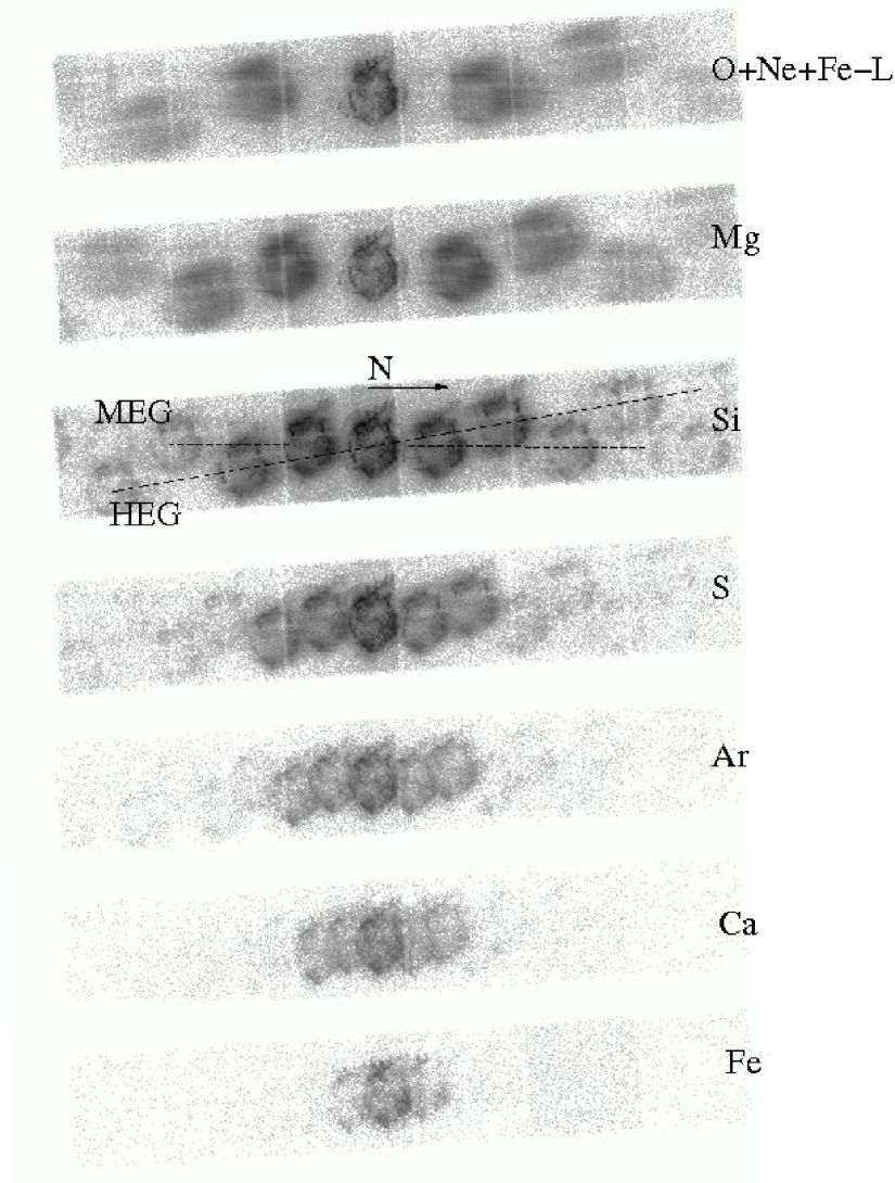
Figure 1: HETG data of Cas A: images of the different line bands. Grating dispersion axes and north direction are marked in the Si-band image. Note the smeared out dispersed-order images, especially in the O+Ne+Fe-L band, due to multiple lines and velocity shifts which, however, do not affect the central, zeroth-order image.

Figure 1 shows the non-dispersed (zeroth-order) image of Cas A at the center of each panel and dispersed images in different energy bands that contain predominately He- and H-like ions, and in the case of Fe also Li- and Be-like ions: O+Ne+Fe-L (0.65–1.2 keV), Mg (1.25–1.55 keV), Si (1.72–2.25 keV), S (2.28–2.93 keV), Ar (2.96–3.20 keV), Ca (3.75-4.00 keV) and Fe-K (6.30–6.85 keV). The Si-band image also indicates the two dispersion axes of the MEG and HEG, which are rotated against each other by $\sim 10\arcdeg$. The Cas A X-ray spectrum is dominated by Si and S lines and these bands produce the clearest dispersed images. The dispersion angle $\theta$ defines the location of the dispersed photon and varies nearly linearly with wavelength $\lambda$, $sin\theta=m\lambda/p$, where $m$ is the order of dispersion and $p$ is the period of the grating. Thus, the dispersed images in the longer wavelengths (O+Ne+Fe-L band) are spread out furthest across the spectroscopy CCD array, while in the shorter wavelength (Fe-K band) the images stay tight to the zeroth-order. Because of this, the longer-wavelength images are more sensitive to velocity gradients and distortions are more prominent, as indicated by the larger smearing seen in the top two panels. The O+Ne+Fe-L image is additionally confused due to the many lines in this band (e.g., Fe-L lines and the O Lyman series; see Bleeker et al., 2001), and a larger relative contribution by the continuum.

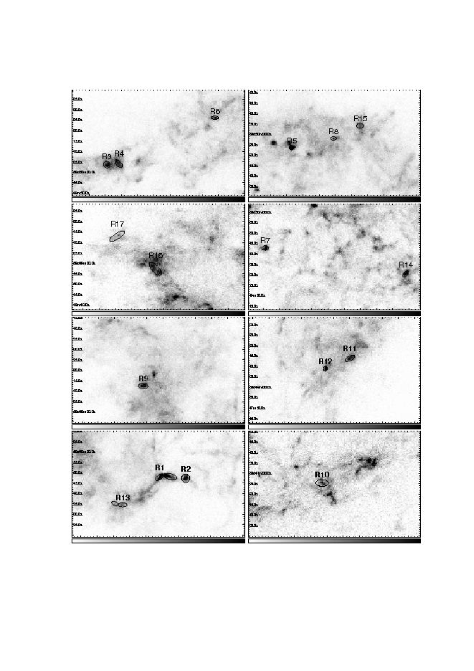
Figure 3: Close up of the regions used in the analysis of HETGS Cas A data. Note that the grayscale dynamic range is not the same for all the sub-plots. Some of the regions have been covered with two elliptical regions to follow the HETGS extraction path (see Appendix A).

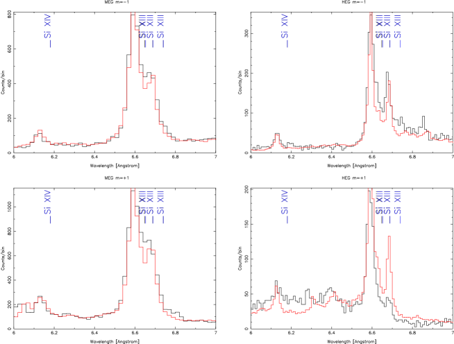
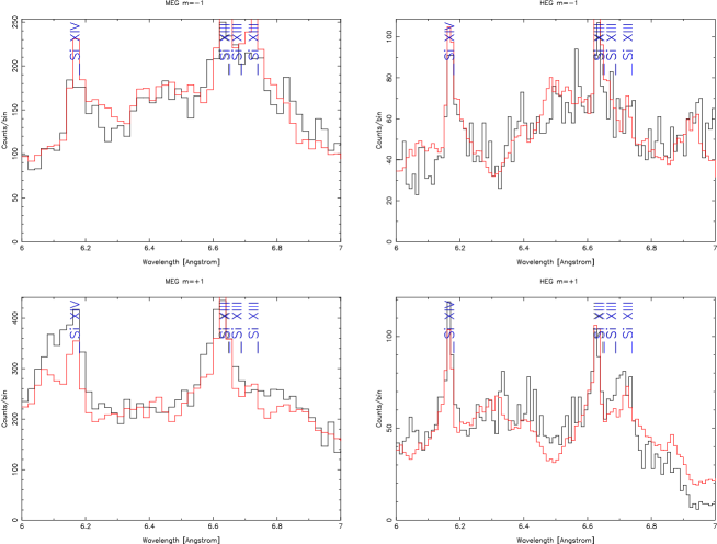
Figure 4: Examples of HETGS spectra of the Si band encompassing four Si lines used in Cas A analysis. The upper four panels show the MEG$\pm 1$ (left) and HEG$\pm 1$ (right) spectra from region R1. The model is plotted with the red line. The nominal positions of Si lines are marked at the top of each panel. For region R1 the observed lines are shifted to lower wavelength, so this region is an example of a blue-shifted region. The lower four panels similarly show the spectra from region R9; this region has a very high Si XIV to Si XIII ratio. Region R1 is also an example of a strong, clear line profile produced by a well isolated clump and little of velocity smearing, whereas from region R9 the line profiles are messy due to lower contrast between the clump and the surrounding medium and possible velocity smearing.

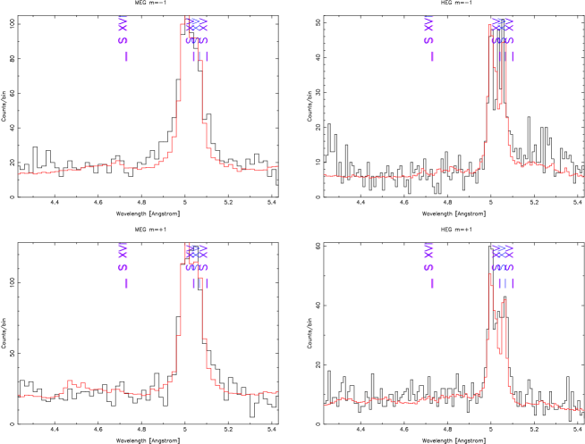
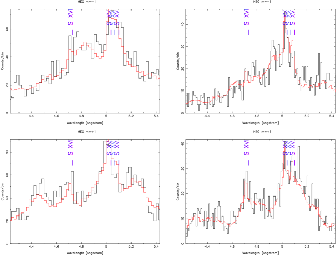
Figure 5: Examples of HETGS spectra of S band encompassing four S lines used in Cas A analysis. The upper four panels show the MEG$\pm 1$ (left) and HEG$\pm 1$ (right) spectra from region R1. The lower four panels similarly show the spectra from region R9. As in the previous plots, the model is plotted with a red line. The nominal positions of S lines are marked at the top of each panel.

Figure 2 shows the regions in the image of Cas A selected for this study. These regions have a morphology and brightness that allow the reliable measurement of line fluxes and centroids. They are spatially narrow along the dispersion direction (north-south) and sufficiently isolated above the local, extended background emission to provide a clear line profile. Figure 3 shows close-ups of these regions. For each region we concentrated on the four strongest dispersed spectra: the MEG +1 and $-1$ orders and the HEG +1 and $-1$ orders. Because of their dominant emission we use the He- and H-like transitions of Si and S lines for the analysis of velocity and plasma structure in Cas A. For typical SNR plasma densities the He-like triplet of the Si and S line shows strong forbidden ($f$) and resonance lines ($r$) and a comparatively weaker intercombination line ($i$). We, therefore, jointly fit our four HETG spectra (MEG$\pm 1$ and HEG$\pm 1$) with a model consisting of 4 Gaussians (representing 3 He-like lines and 1 H-like line for each element) and a constant that accounts for the continuum level (for more details see Appendix A). Figure 4 shows the four sets of Si spectra from region R1, the brightest of the 17 regions, and from region R9 which has the most prominent Si XIV line. Figure 5 shows similarly S spectra from these two regions. In the fit we allow only the centroid of the $r$-line to be a free parameter, while the other three centroids are tied to it, so the relative centroids are fixed, but the template is allowed to slide. We also assume that a single velocity is present in each Cas A region, so all 4 Gaussians have frozen narrow widths. In other words, if there is no velocity structure in a region, the chosen Gaussian width would be the narrowest profile for that spatial structure. In addition, the flux ratio of the $f$-line to the $i$-line (so-called R-ratio) for the Si triplet is tied to be 2.63, suitable for the very low density regime of the Cas A plasma (e.g. Porquet et al., 2001). Similarly, the $f$-line flux is tied to be 1.75 times the $i$-line flux for the S triplet (e.g. Pradhan, 1982).

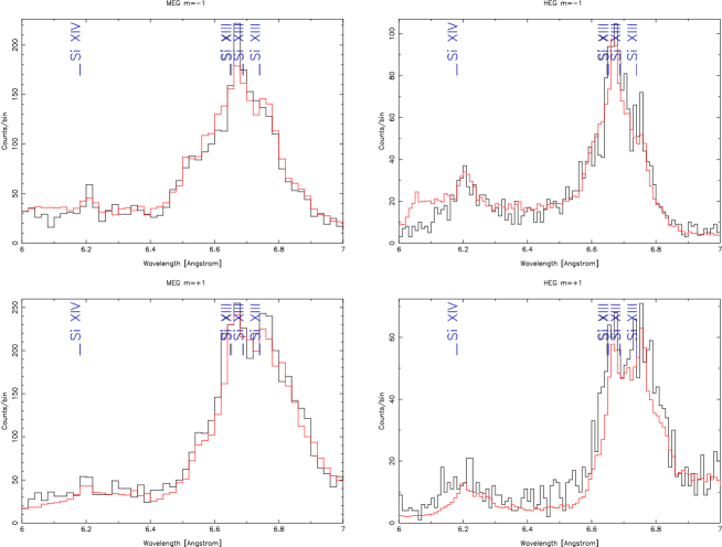
Figure 6: Example of velocity-smearing in region R15 due to a velocity gradient in the dispersion direction (see also Fig. 15(d)). Note that for both the MEG and HEG spectra the $-1$ order (upper plots) is narrower and more peaked than the +1 order (lower plots). As in previous plots, the model is plotted with a red line. The nominal positions of the Si lines are marked at the top of each panel.

To derive accurate Doppler shifts from measuring line centroids we used HEG and MEG spectra binned to 0.01 Å and 0.02 Å, respectively. Our Gaussian fits are not sensitive to measure velocity dispersion as done in the case of E0102–072 (Flanagan et al., 2004), where topographical changes in the dispersed image between positive and negative orders were used to determine intrinsic bulk motions. The RMFs we use in the fitting of Cas A HETG spectra only include broadening due to spatial structure and do not include any further velocity structure degrees of freedom in the quantitative fitting. But we can qualitatively distinguish regions with more or less velocity structure present. Among the line profiles from our 17 regions we find two qualitative types: 1) a narrow profile, where the $r$ and $f$ lines are clearly resolved and shifted due to the region’s bulk motion along the line of sight, and 2) a smeared profile, where one of the grating orders appears broadened due to high-velocity motions within the region relative to its center of mass that causes distortion of the dispersed images along the dispersion direction. For each region the type of the line profile is indicated in Table 1; Figure 4 shows an example of a double-peak profiles, and an example of a clearly smeared spectral profiles is shown in Figure 6.

3.1 Line Dynamics - Doppler Shift Measurement

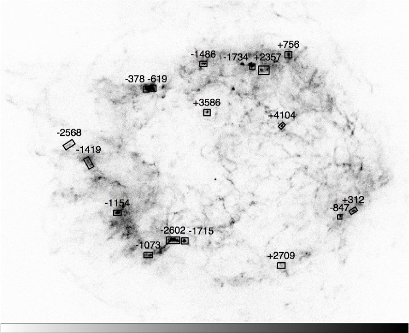
Figure 7: Doppler velocity values in  km s^-1 for individual Cas A regions. The south-east SNR regions measured here are all blue-shifted, while extreme red-shifts are seen in the north-west of the SNR.

Results of Si line measurements and derived Doppler shift values are summarized in Table 1. The spatial distribution of Doppler velocities is shown in Figure 7. Derived values range between $-2500$ km s^-1 to $+4000$ km s^-1. The measured velocity shifts for Si and S (not listed here) are similar (see Fig. 8). This is not surprising since they arise from the same nucleosynthesis layer, and have been found to have the same spatial distribution (Hwang et al., 2000; Willingale et al., 2002). The uncertainties in derived velocities depend, besides on the intrinsic energy resolution of the HETGS, on the number of counts detected in the line and the errors associated with estimates of the continuum contribution. For the Si line the statistical errors for the Doppler shift, based on fit confidence limits, range range within 200 km s^-1 for all regions except for regions R10 and R17 which have errors of 650 km s^-1 and 360 km s^-1, respectively.

The HETGS derived velocities of our 17 Cas A regions are combined with their spatial location on the sky to graphically indicate their 3D location and velocities, as shown in Figure 8. Our measured Doppler velocity is plotted on the y-axis and the x-axis value is the 2D sky radial displacement of the region from the expansion center of Cas A on the sky given by Reed et al. (1995). A factor of $0.032\arcsec\pm 0.002\arcsec$ per  km s^-1 is used to relate velocity to spatial location by minimizing (by eye) the shell width needed to enclose most of the data points (dotted lines.) The velocity center for the shells of +770 km s^-1 is taken from Reed et al. (1995). For a distance to Cas A of 3.4 kpc (Reed et al., 1995) our factor corresponds to a fractional expansion rate of $(0.19\pm 0.01)$ % per year. The forward shock location at 153″ and the mean reverse shock location at 95″, as determined by Gotthelf et al. (2001), is also indicated.

3.2 Line Diagnostics - Flux Ratio Measurements

One advantage of the high-resolution grating spectra of our Cas A regions over lower-resolution CCD data is that we can investigate the plasma state of individual regions using individual emission lines. The He-like K-shell lines, like those of Si and S present in Cas A, are the dominant ion species for each element over a wide range of temperature (e.g. Paerels & Kahn, 2003). From the He-like triplet, the ratio of the forbidden ($f$) and resonance ($r$) lines is a useful diagnostic for electron temperature (e.g., the G-ratio $=(f+i)/r$, Porquet et al., 2001), especially since the lines are from the same ion, which reduces dependence on the relative ionization fraction. Lines from different ions of the same element are also useful because they eliminate the impact of uncertainties in abundance, so e.g. the ratio of the H-like to He-like Si lines in conjuction with the G-ratio of the He-like lines can give an accurate measurement of the progression of plasma ionization.

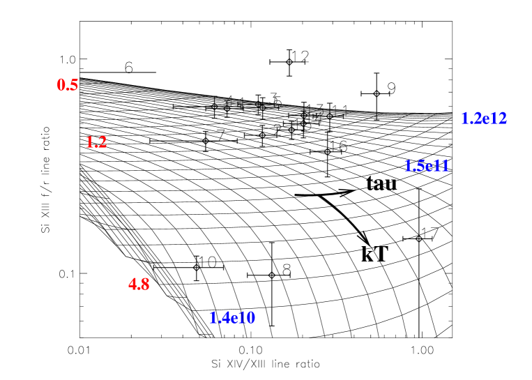
Figure 9: Si line ratios overlaid onto a NEI grid. Upper panel shows the full range of values for all the regions (region R6 is located off the graph), and the lower panel zooms in on the cluster of values in the upper region of the graph. Temperature, $kT_{e}$, increases along the lines which go generally from upper-left to lower right. Ionization time, $\tau$, increases along the lines which are nearly horizontal at left and move to the upper-right ending at the high-$\tau$ limiting asymptote. A few $kT$ values are labeled in red, while some $\tau$ values are labeled in blue.

To determine accurate Si line flux ratios from our data, we fixed the modelled line locations based on our nominal binning and fits described above, and then re-fitted HETG spectra using coarser-bin with modified errors. This procedure, described in Appendix A, is less sensitive to differences between the shape of the analysis RMF and the velocity-modified line shapes. The resulting Si $f/r$ and Si XIV/XIII line ratios are listed in Table 1. We also calculated the expected line ratios, employing the non-equilibrium ionization collisional plasma model with variable abundances, VNEI (Borkowski et al., 2001) in XSPEC with vneivers version 1.1, which uses updated calculations of ionization fractions from Mazzotta et al. (1998). We then used these model grids to map our measured line ratios to equivalent plasma temperature $kT_{e}$ and ionization timescale $\tau=n_{e}t$. Figure 9 shows the distribution of $kT_{e}$ and $\tau$ for the 17 Cas A regions. The point for region R6 falls outside the displayed ratio range because its Si XIV/XIII ratio has an extremely low value. The temperatures range between 0.4 to 5 keV, with the majority of regions having a temperature between 0.7 and 1.0 keV; the distribution of plasma temperature is shown more clearly in Figure 10. The ionization timescale ranges between $10^{10}$ and 4$\times 10^{11}$ cm^-3 s. The measured values for region R9 and R12 fall off of the grid in Figure 9 because of their extremely high $f/r$ line ratios. To assign $kT_{e}$ and $\tau$ values to region R9, we used the lower error limit which falls within the NEI grid. For region R12, we used a value within a 20–30% discrepancy of the lower limit. Thus, the derived values (e.g., $n_{e}$, $t_{\rm shock}$) for regions R6, R9 and R12 should be taken with some leeway.

3.3 Zeroth-order Spectra - Density and Abundance Measurements

In addition to the dispersed data, we also use the non-dispersed data (from the central ACIS chip seen in Fig. 1) to obtain information on the abundances and emission measure for the individual regions. Obtaining information on global plasma parameters such as electron density and elemental abundance requires comparing line to continuum in the spectra, and also knowing what are the contributions to the continuum. The dispersed spectra will have contribution from superimposed lines and continua from other image regions, although the superimposed lines would not have the right energies (see Appendix A for more details). Because of this confusion dispersed data are not reliable for measuring line to continuum ratio. Therefore, to determine these plasma parameters for each of the 17 regions, we fitted the non-dispersed zeroth-order spectra with a single VNEI plasma model (Borkowski et al., 2001), which allows for varying elemental abundances. In these fits we fixed the $kT_{e}$ and $\tau$ values for each region according to the values derived from HETG line ratios. Cas A spectra, even of isolated features, are very complex and four spectral components have been identified (e.g. DeLaney et al., 2004). These four spectral components are rarely present at the same location and most of DeLaney et al. (2004) knots show characteristics of a single type, with some showing mixed characteristics. To avoid complications due to varying column density ($N_{\rm H}$) and continuum levels we ignore the low-energy part of the spectrum and consider only the range between 1.1 and 8.0 keV encompassing K-shell lines of Mg, Si, S, Ar, Ca and Fe-K. An O-rich plasma is often employed when describing Cas A ejecta (e.g. Vink et al., 1999; Hughes et al., 2000; Laming & Hwang, 2003), since optical observations showed that ejecta in Cas A are deficient in H and rich in O and O-burning products (e.g. Chevalier & Kirshner, 1978). We, therefore, assume that O dominates the continuum emission, and that O provides many of the electrons instead of H and He, as in the typical solar abundance plasma. Thus, we fix the O abundance to be a factor of 1000 higher than the solar value. The results are, of course, not very sensitive to the exact O overabundance factor. We also fix $N_{\rm H}$ to 1.5$\times 10^{22}$ cm^-2, which is found to be an average value across the SNR (e.g. Vink et al., 1996; Willingale et al., 2002). In the fit we allowed the normalization and the abundances of Mg, Si, S and Ca to vary. The Ar line is not included in the VNEI model (vneivers version 1.1), so we use a Gaussian to model the Ar emission. The prominent Fe-K XXV line is only present in regions R9 and R16, which is not surprising since they are located in the area rich with Fe called the ”Fe cloud” (Hwang & Laming, 2003).

We tried different approaches for handling the red-shift parameter $z$ in fitting these CCD data. We first froze the $z$ values to those derived from the HETGS data, but the resulting fits were not acceptable, showing a clear mismatch between data and model line peaks. These offsets are likely ACIS gain uncertainties and other calibration errors in the CCD response. Reasonable fits were obtained by manually adjusting the $z$ values separately for each data set; the values used varied between $-0.005$ and $+0.035$.

Table 2 lists parameters measured from the zeroth-order spectral fits of the 17 regions. The first column lists the region emission volume $V_{R}$, which was taken to be a triaxial ellipsoid whose 2D-projected area corresponds to the spectral extraction region shown in Figure 3 with radii $a$ and $b$. For the third axis along the line of sight we take the average value of the two observed axes, $c=(a+b)/2$; the volume of the region is then:

$$V_{R}={4\over 3}\pi\ a\ b\ c.$$ (1)

The second column lists the normalization factor (“norm”) used in the VNEI model, e.g.,

$$X_{\rm norm}\ \equiv\ {{10^{-14}}\over{(4\pi d^{2})}}\ \int n_{e}n_{H}\ dV.$$ (2)

Note that the tabulated norm here assumes that the model oxygen abundance is set to 1000. The rest of the columns list the abundance ratios with respect to oxygen for the elements Mg, Si, S and Ca. Using the equations given in Appendix B we derive and tabulate in Table 3 some relevant physical parameters for the regions based on these fit results: the region’s electron density, the total mass of plasma in the region, the time-since-shocked for the region $t_{\rm shock}=\tau/n_{e}$, in units of years, and finally the fraction of oxygen by mass per region.

4 Discussion

4.1 Doppler measurements in Cas A

The measurement of Cas A Doppler shifts in the X-ray band was first conducted with the Einstein X-ray Observatory using the Focal Plane Crystal Spectrometer (FPCS) (Markert et al., 1983). The bulk velocities of two regions of Cas A, the SE and NW halves, were measured using the line centroids of the resolved Si and S triplets. These observations found a velocity broadening and asymmetry in the X-ray emitting material, with the NW region having more red-shifted emission, and the SE region of the remnant having more blue-shifted emission. Markert et al. (1983) suggested that the asymmetry could be the result of an inclined ring-like distribution of Cas A material, possibly influenced by the distribution of the mass-loss material of the progenitor. Our HETGS spectra of individual Cas A filaments reconfirms this global asymmetry trend. The SE regions of the SNR appear to be mostly blue-shifted and the regions in the NW have the extreme red-shifted values. The asymmetry was also found with moderate spectral resolution of ASCA (Holt et al., 1994). The ASCA observations provided a velocity map on the spatial scale of 1′ and were derived using the Si line centroids at the CCD resolution.

Doppler velocity maps with a much finer spatial resolution were produced using Chandra (Hwang et al., 2001) and XMM-Newton observations (Willingale et al., 2002). Hwang et al. (2001) used the Si XIII resonance (1.865 keV) and Si XIV Ly$\alpha$ (2.006 keV) line centroids to derive the velocity shifts on a 4″ spatial scale. While most of the SNR showed velocities between $-1500$ and $+1500$ km s^-1, extreme velocities of $-6000$ km s^-1 were found in the SE region, including the region of our R1, R2, R9 and R13 for which HETGS data imply velocities between $-2500$ and $-1000$ km s^-1. This discrepancy is not too surprising. Although Hwang et al. (2001) argued that they can ignore the ionization effects on the Si He$\alpha$ centroid to a reasonable approximation, they note that high spectral resolution measurements are more desirable to measure the energy shifts directly from resolved rather than blended lines. Indeed, their Chandra data do not resolve the Si XIII triplet, and even the Si XIV and Si XIII Ly$\alpha$ lines are not fully resolved, introducing some level of uncertainty in line centroid measurement. The most recent results from the 1 Ms Very Large Project (VLP) Chandra data show values more consistent with our HETGS data (Stage et al., 2006), but even here absolute gain calibration accuracies for the CCD may only be good to 0.5% or 1500 km s^-1.

XMM Doppler maps of Si, S and Fe lines by Willingale et al. (2002) show a smaller range in velocity than the Si velocity map of Hwang et al. (2001) and, thus, values that are at a glance closer to our values in Table 1. The XMM data have been binned to a $20\arcsec\times 20\arcsec$ spatial grid and the spectra were fit with two thermal NEI components representing the ejecta and the shocked component, each with a separate energy shift. The Doppler shift values derived in this way will depend on the ability of the NEI spectral model to predict the line blends combined with the uncertainties in the gain calibration of the detectors. In comparison to our results, it is obvious that some of the errors in their Doppler shift values are produced because of the spatial averaging over a variety of features with very different velocities. For example, in the NW region the Doppler velocity map of Willingale et al. (2002) has a smooth distribution of red-shifted values with a 1000 km s^-1 or so dispersion, whereas our regions R5 and R6 in that part of the SNR show significantly blue-shifted values of around $-1500$ km s^-1, as well as red-shifted velocities with 1000 km s^-1 difference between regions R8 and R15. Willingale et al. (2002) find that the velocity patterns for S are very similar to those for Si; our measured Si and S velocities agree with this. The Fe-K velocities, however, exhibit higher velocities than those of Si and S; this has also been found with the 1 Ms VLP Chandra observations of Cas A (Stage et al., 2006). Note that our two regions showing Fe-K emission, R9 and R16, are located in the middle (R9) and outside (R16) the range of other regions (see Fig. 8). Unfortunately, our HETGS data do not have enough counts in the Fe-K band to measure shifts in the Fe energy; deeper HETGS observations might yield Fe-K velocity measurements with 500 km s^-1 errors, provided the required narrow features are present.

Probably the best demonstration of the magnitude of the difference between the CCD and HETGS measured Doppler shifts is given by comparing the estimated shock expansion rate in Cas A. DeLaney & Rudnick (2003) derived forward shock expansion measurements of 0.21% per year using transverse velocity measurements of Cas A knots using Chandra CCD data. DeLaney et al. (2004) compared their transverse velocities (3100–3900 km s^-1) with that of Willingale et al. (2002) (1000–1500 km s^-1) and Hwang et al. (2001) (2000-3000 km s^-1) obtained from Doppler measurements using CCD spectra, and graciously ascribe mismatch to possible projection effects of the asymmetric remnant. However, our Doppler measurements imply an ejecta expansion of 0.19% per year, consistent with the DeLaney & Rudnick (2003) and DeLaney et al. (2004) value. This supports their suggestion that there might be a dynamic coupling between forward shock and ejecta, and they are both part of one homologously expanding structure. Note that Vink et al. (1998) derived an expansion rate of 0.2% per year by comparing the ROSAT and Einstein X-ray images from two different epochs.

The region R17 is the only region outside our reverse-shock/forward-shock range and its location at a large radius from the expansion center puts it outside the nominal forward shock 3D radius as seen in Figure 8. This is also a characteristic of the optical FMKs, which are found mostly in the NE part of the remnant, with many of them located along the jet. Our region R17 is located in the base of the jet region (see Fig. 2), and its velocity indicates that it indeed might be part of the jet feature.

4.2 Plasma properties

Beside the Doppler shifts, plasma temperature and ionization timescale are the two other plasma parameters derived directly from our HETGS analysis. Early observations of Cas A in X-rays identified two distinct plasma components — the cold component with temperature around 0.6 keV, and the hot component with temperature up to 4 keV (e.g. Becker et al., 1979), and they have been confirmed with newer observations (e.g. Vink et al., 1996; Willingale et al., 2002). The cooler component is associated with the reverse shock traveling through the expanding ejecta, and the hotter component is associated with the forward shock propagating into the circumstellar material. Plasma temperatures derived from our HETGS data have values mostly around 1 keV. Therefore, most of our regions have been heated up by a reverse shock propagating inward into the supernova ejecta. There is no significant pattern to the variation in the temperature across the SNR, as shown in Figure 10. The exceptions are regions R8, R10 and R17 which do have temperatures of 4–5 keV, several times higher than most other regions. Regions R8 and R10, which also share similar velocity, could, therefore, be associated with circumstellar material and the forward shock. Region R17 could be an X-ray counterpart of the optical FMKs found in Cas A jet. Willingale et al. (2002) derived a map of ionization timescale for the cool plasma component in Cas A, which shows some variation across the surface of the SNR, but most of the SNR has $\tau$ values larger than $10^{11}$  cm^-3 s. For our 17 regions we also find little variation, most of the regions have $\tau$ around a few $10^{11}$ cm^-3 s. The exception are, again, only regions R8 and R10, as shown in Figure 10, which have ionization timescale up to an order of magnitude smaller.

Information on density and abundances for the 17 Cas A regions is derived in conjunction with the zeroth-order data. The zeroth-order spectra are reasonably fit with a single VNEI model with fixed temperature and ionization timescale, certainly well enough for our primary purposes here to establish relative abundances. An example spectrum is given in Figure 11 for region R9. In the 1.1 and 8 keV range the spectrum shows a weak Mg lines, strong Si, S, Ar and Ca lines, and a weaker Fe-K line, and shows reasonable agreement between the data and the model for the continuum part of the spectrum. Note that a low-energy “up-turn” is also present due to emission from Fe-L lines and this part of the spectrum, below 1.1 keV, was not used in the fit. The Si XIII Ly$\beta$ line at 2.18 keV is generally under-fit in the spectra; this is likely due to several calibration issues each at the 10-20% level (e.g., Ir contamination is not included in the HRMA model, there are possible zeroth-order HETG calibration errors, CCD gain offsets are coupled with steep ARFs.) Future work using the higher-count Cas A VLP data set and including these calibration effects could usefully extract the He-like Ly$\beta$ line flux allowing associated diagnostic ratios (Porquet et al., 2001) and possibly indicating charge-exchange processes (Pepino et al., 2004).

Electron density for each of the regions, derived as described in Appendix B, is listed in Table 3. The $n_{e}$ ranges from around 20 to 200 cm^-3 and it seems to have higher values for the blue-shifted regions. A factor of 5 density difference has been suggested between the front and the back of Cas A (Reed et al., 1995). The time since individual Cas A regions have been shocked, given by $t_{\rm shock}=\tau/n_{e}$, is also listed in Table 3. These times vary significantly from region to region and it seems that the red-shifted regions have been shocked more recently compared to the regions on the front side which have generally larger $t_{\rm shock}$ values (regions R6, R9 and R12 have extreme values that should be taken with caution), as shown in Figure 12. However, these values could be the result of density differences between the front and the back side of the SNR. We do not find any correlation between $kT_{e}$ and $t_{\rm shock}$ or $n_{e}$ and $\tau$ that would indicate a possible electron-ion equilibration occurring in our 17 regions.

The other parameters listed in Table 3 are the total mass and the fraction of O mass per region. These values should be taken with caution, because we assumed in our fit that continuum is dominated by O. Note also that our total mass estimate does not include Fe or Ar since they are not included in our NEI model, so the $M_{\rm total}$ values could be somewhat modified when these are included. The O mass fraction ranges from 0.82 to 0.97, thus confirming that, under our assumptions, O is the dominant element in these Cas A ejecta features. Cas A is an O-rich SNR, as indicated by optical observations, and this leads to the further assumption that perhaps there is also a lot of O in the regions between the bright Si knots that we see. For example, Laming & Hwang (2003) estimate that a density enhancement of around 2 coupled with the presence of the Si-Ca metals would allow these knots to stand out even though surrounded with a pure oxygen plasma. This may be another reason that the O-band dispersed image appears so smeared out and that we do not detect clear O-lines in our HETGS data: there is O emission everywhere within the shocked ejecta region so we do not see discrete O filaments or clumps like those in the Si and S band images.

In order to test the suggestion by Laming & Hwang (2003) about the wide-spread presence of O emission, we make a few simple estimates. Table 3 shows the mass fraction of oxygen to be 0.82 in region R1. Under the assumption that the entire SNR volume within a radius of 100″ and 130″, for example, is filled with oxygen of the density projected for R1, the total mass of oxygen would amount to 85$M_{\odot}$. Earlier studies imply a mass of 4$M_{\odot}$ for the entire ejecta at most (e.g. Vink et al., 1996). Thus, our results seem to either overestimate the oxygen density or the density of that particular region is not representative for such a large volume. Even if we further assume that the density in R1 is enhanced with respect to the ambient medium by the factor of 2 to 5 (Reed et al., 1995), we would wind up with 40 to 16$M_{\odot}$ of oxygen under uniform conditions. Introducing a density gradient to the ejecta, such as a rise in density towards the center of the remnant, gives an increase of at least another factor of 2. Therefore, such simple estimates do not seem to support the Laming & Hwang (2003) assumption. Alternatively, Willingale et al. (2003) derived a filling fraction of 0.009 for the ejecta component by assuming a pressure equilibrium between hot and cool plasma components, which lead to an electron density range of 40–90 cm^-3, similar to our values. Adding such a factor to our estimate above would then allocate much of the metals and oxygen into spaghetti-like filaments requiring a total mass of order 1$M_{\odot}$. This value represents a more reasonable contribution to a total oxygen mass of 2.6$M_{\odot}$ suggested by Vink et al. (1996).

5 Summary

High-resolution HETGS observations from the young SNR Cas A yield unprecedented kinematical X-ray results for a few bright SNR regions. These observations show that high-resolution X-ray spectroscopy is catching up with that in optical, IR and UV bands in its ability to measure velocities and add a third dimension to the data. Unambiguous Doppler shifts are derived for these selected regions, with the SE region of the SNR showing mostly blue-shifted values reaching up to $-2500$ km s^-1, and the NW side of the SNR having extreme red-shifted values with up $+4000$ km s^-1. This global asymmetry is consistent with previous lower spatial or spectral resolution X-ray observations. From our Doppler measurements we derive ejecta expansion of 0.19% per year, supporting suggestion of DeLaney et al. (2004) that there might be a dynamic coupling between the forward shock, that is expanding at the same rate, and the ejecta.

Plasma diagnostics using resolved Si He-like triplet lines and Si H-like line shows that most of the selected regions in Cas A have temperatures around 1 keV, consistent with reverse-shocked ejecta. However, two regions, R8 and R10, with significantly different temperature of $\sim 4$ keV, might be part of the circumstellar material. Similarly, the ionization age does not vary considerably across the remnant, except for the two above mentioned regions, which have an order of magnitude lower ionization timescale. One of the regions, R17, is located outside the forward shock boundary and also has a high plasma temperature, both suggesting that this region is part of the Cas A NE jet feature.

The analysis of HETGS data was complemented by the non-dispersed CCD ACIS spectra from the same observation, which allowed us to derive the electron density of the X-ray emitting ejecta and the elemental abundances of Mg, Si, S and Ar in our 17 regions. The electron density varies from 20 to 200 cm^-3 and does not show any correlation with ionization timescale. The derived elemental abundances of Mg, Si, S and Ca are consistent with O being the dominant element in the Cas A plasma.

Appendix A Filament Analysis

A.1 Filament Analysis Scheme

The “filament analysis” we used for Cas A HETGS data is very similar to the standard analysis of dispersed grating data from a point source, in that it produces a one-dimensional PHA file with associated ARF and RMF for each grating and order. The two main additions to the standard processing that adapt it to extended, filament-like sources are described briefly below.

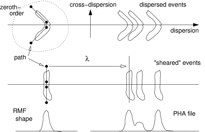
Figure 13: Filament analysis schematic. A path is defined and used to straighten a filament-like feature seen in zeroth-order. A ”shearing” process is carried out to translate each event location in the dispersion direction by an amount given by its cross-dispersion coordinate and the path. An effective RMF and corresponding PHA file are created and can be used in data analysis.

First, adjustments to the event locations are applied to effectively straighten the filament-like source perpendicular to dispersion while retaining wavelength accuracy; specifically, the following steps are carried out. The shape of the source in zeroth-order is manually traced by a piecewise-linear path that is saved as a set of vertices. The vertex locations are then transformed into coordinates aligned with the dispersion and cross-dispersion direction of the particular spectra (HEG or MEG) being extracted, see top diagram in Figure 13. Each event, in both the zeroth-order and the dispersed orders, is then translated along the grating dispersion direction by an amount equal and opposite to the path offset at that same cross-dispersion location. This ”shearing” causes the zeroth-order and any dispersed line-images of the feature of interest (FOI) to become narrower along the dispersion coordinate, see middle diagram of Figure 13. A PHA file of counts per dispersion bin is then created in the usual way by projecting the events along the dispersion axis, see bottom diagram Figure 13. Because the dispersed features are effectively narrowed, the ability to detect and resolve discrete lines from the feature is improved.

Second, a companion response matrix, RMF, is created based on the observed, sheared zeroth-order events. For each wavelength in the RMF, a subset of events are selected using the available non-dispersive energy reported by the CCD detector and the expected response histogram is created and stored with appropriate offsets in the RMF. Operationally this is similar to the effect of the rgsxsrc convolution model available in XSPEC for use with XMM-Newton Reflection Grating Spectrometer data.

This is just one approach to extended source grating analysis (Dewey, 2002) and has the advantage of producing familiar PHA files which can be analyzed with standard software like ISIS (Houck, 2002). Note, however, that it is fundamentally an approximation to a fully multi-dimensional, spatial-spectral method and so will necessarily have limitations; some of these are implicit in the considerations and techniques described in the following sections.

A.2 Treatment of Spectral Continua

In addition to line emission from the narrow FOI, there is also continuum emission from the feature, as well as line and continuum emission from other parts of the extended source. These give rise to a continuum component in the observed PHA spectrum which we discuss and estimate here.

The observed count rate at a given location on the detector is given by a 3D integral over the source flux as a function of wavelength and position on the sky (see eq.(49) in Davis, 2001). This integral includes the grating response function, which has the property that the location of a dispersed photon includes a continuous dependence on the photon’s wavelength. Thus, for a given position on the detector there is a set of sky locations and corresponding wavelengths which all contribute detected counts in this same location. This is in contrast to the point-source case where the point source introduces a delta function in the integral and preserves a one to one mapping of source wavelength to dispersed location in each grating-order. The continuum counts seen within a bin in the PHA distribution file will then consist of the sum over the spatial regions along the dispersion axis weighted by their flux at the grating-equation-allowed wavelengths. Equivalently, the resulting spectrum includes not only the true continuum from the FOI, but the overlapping, shifted spectra from all regions along the dispersion axis.

In practice, the integral may be effectively truncated, e.g., if the spatial extent of the source is moderate. In addition, even for very extended sources, the inherent energy resolution of the detector can be used to truncate the integral to a limited range in pulse-height, reducing the artificial continuum level. In this case, the observed continuum will be of order a factor of $R_{g}/R_{\rm CCD}$ greater than the true FOI continuum level, where $R_{g}$ and $R_{\rm CCD}$ are the effective resolving powers of the grating and order-sorting detector, respectively. Note that $R_{g}$ for a given feature varies like $1/E$ and $R_{\rm CCD}$ varies roughly like $\sqrt{E}$, where $E$ is the energy; thus, the $R_{g}/R_{\rm CCD}$ ratio varies approximately like $E^{-1.5}$ (or $\lambda^{1.5}$). This is a small variation, of order $\pm$12% over the 6–7 Å range for Si lines.

As a demonstration of this, a simple MARX simulation was made consisting of a $\approx 4.0\arcsec\times 10\arcsec$ rectangle emitting at 1.865 keV embedded in a disk of emission 100″ in radius having a uniform spectrum from 1.2 to 2.8 keV. Figure 14 shows the CCD spectrum extracted from the zeroth-order (e.g., the rectangular region) and the spectrum extracted from the MEG dispersed first order. The effective grating resolving power here is $R_{g}\approx 75$ based on the source full width. For the order-sorting effective resolving power, $R_{\rm CCD}$, the dispersed extraction was performed with a wide pulse-height selection including $\pm 0.15\lambda$, giving $R_{\rm CCD}\approx 3.3$, based on the energy full width. Together these give $R_{g}/R_{\rm CCD}\approx 23.$ In the simulation the equivalent width, EW, of the line is 21.4 keV for the zeroth-order case, and 1.29 keV in the dispersed case; the continuum level is, therefore, $\approx 17$ times larger in the dispersed data set, which is of the order expected from the simple estimate.

A.3 Velocity Effects and Fitting

The features we observe in Cas A show Doppler shifts of up to several thousand  km s^-1. For a simple bulk motion of the emitting region this just produces an overall Doppler shift to the line wavelength which can be readily measured using the filament analysis products. It is also possible that there are velocity variations within the filament itself and this can introduce some complications, especially when carrying out standard $\chi^{2}$-driven fitting.

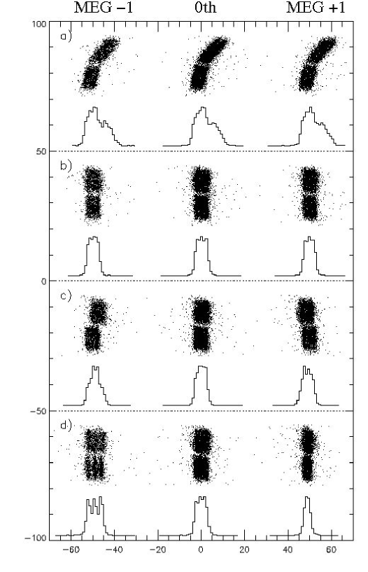
Figure 15: Velocity effects on dispersed line shapes. Each of the four panels here is from a simple MARX simulation and filament analysis, showing close-ups of the minus order (MEG $-1$), zeroth-order (0th), and plus-order (MEG +1) with event scatter-plots and 1D histograms. The top panel (a) shows the original, simulated filament without shearing applied. In (b) all events have been sheared using a simple path; the width of the feature has been narrowed to about 5 pixels wide. In (c) the upper-half of the feature is emitting at a wavelength blue-shifted by 1000 km s^-1 with respect to the lower half. The zeroth-order is unaffected, but the first orders are blurred equally by this velocity variation in the cross-dispersion direction. In (d) the source has a velocity variation along the dispersion direction with blue-shift values of: 0, -500, and -1000 km s^-1. In this case the effect is to broaden the minus order (showing the three individual line sources used to simulate the wide filament) and narrow the plus order to the point that it is actually narrower than the zeroth-order itself; the zeroth-order is unaffected.

In order to study these velocity effects, simple MARX simulations were carried out using a filament source (resembling our region R1) consisting of two sets, upper and lower, of three closely spaced (by precisely 1″) parallel line sources. The two sets were tilted and offset to produce a wide, kinky filament, shown in panel (a) in Figure 15. In the MEG simulations of panels (a) and (b) all the 6 line sources making up the filament all have the same wavelength. These two panels show how the shearing of the filament analysis improves the resolution of the dispersed spectra.

In simulation (c) the upper set of three lines have all been blue-shifted by 1000 km s^-1 demonstrating the effect of velocity variation along the filament. This causes the dispersed projections to be additionally blurred, having a FWHM larger than the (unaffected) zeroth-order. A similar result would arise for the case of turbulent velocity broadening where there would be a range of velocities in all parts of the emitting feature.

The simulation in panel (d) is perhaps the most pathological: here the velocity of the filament varies across the filament, along the dispersion direction. The zeroth-order continues to be unaffected by these velocity effects, and now not only do the the dispersed order projections differ from the zeroth-order, but they are different from each other as well (see HETGS observations of SNR E0102–072, Flanagan et al., 2004).

The effect of these velocity produced changes in the dispersed line profiles is that the RMF created from the zeroth-order is not a good match when there is velocity structure in the feature. For purposes of fitting the line location, the generally peaked nature of both the RMF and the dispersed line peaks leads to reasonable centroid fitting and confidence ranges; however, the formal $\chi^{2}$ values can be large.

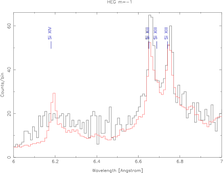
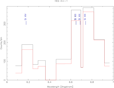
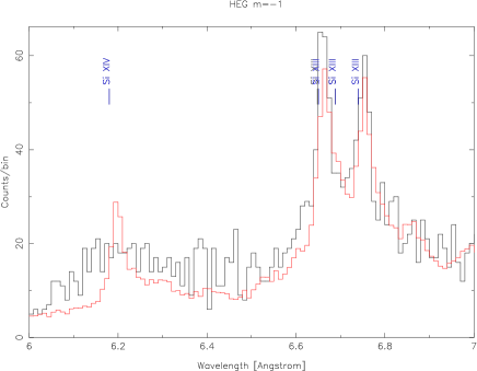
Figure 16: An example of coarse fitting to determine line fluxes. The top panel shows the data and model fit for the HEG m=$-1$ spectrum using our nominal binning; the HEG m=$+1$ and MEG m=$\pm 1$ spectra are simultaneously fit as well but not shown. This fitting allows the centroids to be accurately measured. In the middle panel the data and model (with line centroids fixed) are binned on a coarser custom grid that is aligned with the line locations. Using this coarse binning the spectra are jointly fit with a constant-percentage error term since systematic errors now dominate. In the bottom panel the coarse-fit model and data are shown on the nominal grid; note that the modelled lines have grown.

The mismatch of the zero-velocity line shape used in our RMFs is more problematic when measuring the line fluxes. To reduce these mismatch effects we can fix the line locations in the model at the centroid values determined in our nominal fitting and then rebin the data and model to a coarser grid. We use binning of order 10 bins, with bin boundaries located in the regions between the lines. In this way the total counts in a line region are compared between model and data while ignoring line shape differences. Because of the large number of counts in each coarse bin, the errors are now dominated by the approximations of our RMFs and systematic calibration errors between the 4 spectra we are jointly fitting, HEG m=$\pm 1$ and MEG m=$\pm 1$. In place of the usual statistical error, we assign a constant error value to the bins of each coarse spectrum with a value of 4% of the maximum counts in a bin of that spectrum. This produces fits in which the fluxes of the lines are better estimated, as we confirm by examining the fits when data and coarser-fit model are re-plotted to our nominal binning, as demonstrated in Figure 16.

Appendix B Converting VNEI Parameters to Physical Units

This appendix summarizes the conversion of model parameter values into physically meaningful plasma quantities, e.g., the electron density, $n_{e}$, and the mass of each element present, $M(Z)$. A variety of models in the XSPEC library, including the VNEI model we use in this work, digest the properties of the emitting plasma into a normalization factor, $X_{\rm norm}$, and a set of relative elemental abundances, $X_{A}(Z)$. In addition to these, two other source parameters are needed: the source distance,

$$d\ [{\rm cm}]=3.1\times 10^{21}\ d_{\rm kpc},$$ (B1)

and the volume of the emitting region,

$$V_{R}\ [{\rm cm^{3}}]=V_{\rm as3}\ (d{{\pi}\over{180}}{{1}\over{3600}})^{3}.$$ (B2)

For convenience the conversion from values in kpc, $d_{\rm kpc}$, and arcseconds³, $V_{\rm as3}$, are shown in these equations.

The actual number fraction of the element $Z$ in the plasma is then given by:

$$f(Z)=X_{A}(Z)\ A_{\rm model}(Z)\ /\ \sum X_{A}(Z)A_{\rm model}(Z),$$ (B3)

where $A_{\rm model}(Z)$ is the reference “solar” number abundance ratio assumed by the model; in our case these are the Anders & Grevesse (1989) values. The parameters, $X_{A}(Z)$, are the usual relative abundance values as input in XSPEC models.

Because we do not assume that hydrogen dominates the plasma, it is necessary for the electron density to be self-consistent with the densities and ionization states of the ions present. The ratio of electron $n_{e}$ to total ion density $n_{i}$ is then given by:

$$({{n_{e}}\over{n_{i}}})\ =\ \sum Q(Z)\ f(Z),$$ (B4)

where $Q(Z)$ is the average number of electrons stripped from the ions of element $Z$, in the range 0 to $Z$. Ideally $Q(Z)$ would be provided by the model; lacking direct access to it, however, we can make a simple approximation to the ionization state of the elements in our O-rich plasma by setting:

$$Q(Z)\ =\cases{Z,&if $Z\leq 9$;\cr Z-2,&for $10\leq Z\leq 16$;\cr Z-10,&if $Z\geq 17$.\cr}$$ (B5)

The electron density can then be calculated as:

$$n_{e}=\sqrt{X_{A}(Z=1)\ (n_{e}n_{H})\ ({{n_{e}}\over{n_{i}}})\ {{1}\over{f(Z=1)}}},$$ (B6)

where $n_{H}$ is the hydrogen density and $(n_{e}n_{H})$ is given by the usual normalization definition

$$(n_{e}n_{H})\ =\ 4\pi d^{2}\ {10^{14}}\ X_{\rm norm}/V_{R}.$$ (B7)

The $X_{A}(Z=1)$ factor is included in case the hydrogen model abundance is set to other than 1.0, e.g., to a small value like 1$\times 10^{-9}$ for a pure metal plasma. The density of element $Z$ is then given by

$$n(Z)\ =\ f(Z)\ n_{e}\ /\ ({{n_{e}}\over{n_{i}}}),$$ (B8)

and other quantities like the mass or mass fraction can be calculated in a straight forward way using the volume, $V$, and appropriate constants (1 amu = 1.66$\times 10^{-24}$ g and $M_{\odot}$= 2$\times 10^{33}$ g.)

Table 1: Measured and derived parameters for 17 Cas A regions from HEG+MEG spectral fits to Si lines: line velocities, plasma temperature $kT$, ionization timescale $\tau$, and Si line ratios, forbidden to recombination line ratio and XIV to XIII line ratio. We also list the type of line profile in the last column: ”n” indicates narrow, normal, double peaked Si XIII line profile produced by $r$ and $f$ lines, and “sm” indicates smeared line profile due to velocity gradient. Note that for the three regions given in parenthesis the Si ratios are not on the model grid (see Fig. 9) and so the $kT$ and $\tau$ values assigned are approximate.

Region	Velocity	$kT$	$\tau$	Si	Si	Line
	( km s-1)	(keV)	( cm-3 s)	(f/r)	(XIV/XIII)	profile
R1	$-2600\pm 70$	0.77${}^{+0.04}_{-0.04}$	2.1${}^{+2.1}_{-0.8}$$\times 10^{11}$	$0.59\pm 0.05$	$0.07\pm 0.02$	n
R2	$-1715\pm 80$	1.09${}^{+0.24}_{-0.05}$	1.1${}^{+0.4}_{-0.5}$$\times 10^{11}$	$0.44\pm 0.05$	$0.12\pm 0.02$	n
R3	$-380\pm 80$	0.74${}^{+0.07}_{-0.07}$	4.2${}^{+22}_{-2.9}$$\times 10^{11}$	$0.61\pm 0.06$	$0.12\pm 0.03$	n
R4	$-620\pm 150$	0.74${}^{+0.11}_{-0.10}$	2.1${}^{+5.8}_{-1.3}$$\times 10^{11}$	$0.60\pm 0.07$	$0.06\pm 0.03$	n
R5	$-1735\pm 118$	0.77${}^{+0.13}_{-0.07}$	3.6${}^{+5.7}_{-2.1}$$\times 10^{11}$	$0.59\pm 0.07$	$0.12\pm 0.03$	sm
(R6)	$-1490\pm 90$	0.43 ($<1.5$)	3.5$\times 10^{9}$ ($>2$$\times 10^{9}$)	$0.86\pm 0.10$	$0.001\pm 0.027$	sm
R7	$+3585\pm 135$	1.20${}^{+0.20}_{-0.16}$	4.9${}^{+4.3}_{-2.5}$$\times 10^{10}$	$0.41\pm 0.04$	$0.05\pm 0.03$	n
R8	$+2360\pm 140$	4.80${}^{+1.00}_{-1.1}$	2.2${}^{+0.6}_{-0.6}$$\times 10^{10}$	$0.10\pm 0.04$	$0.13\pm 0.04$	sm
(R9)	$-1150\pm 90$	$<1.30$	$>6$$\times 10^{11}$	$0.70\pm 0.17$	$0.54\pm 0.10$	sm?
R10	$+2700\pm 650$	4.30${}^{+0.50}_{-0.20}$	1.3${}^{+0.3}_{-0.5}$$\times 10^{10}$	$0.11\pm 0.01$	$0.05\pm 0.02$	sm
R11	$+310\pm 250$	0.99${}^{+0.06}_{-0.14}$	3.6${}^{+11}_{-1.8}$$\times 10^{11}$	$0.54\pm 0.08$	$0.29\pm 0.06$	n
(R12)	$-850\pm 85$	$>0.81$	$>2.6$$\times 10^{12}$	$0.97\pm 0.13$	$0.17\pm 0.04$	n
R13	$-1070\pm 140$	0.90${}^{+0.25}_{-0.13}$	3.6${}^{+11.3}_{-2.3}$$\times 10^{11}$	$0.54\pm 0.08$	$0.20\pm 0.04$	n
R14	$+4100\pm 170$	0.99${}^{+0.21}_{-0.09}$	2.4${}^{+2.1}_{-1.3}$$\times 10^{11}$	$0.50\pm 0.07$	$0.20\pm 0.05$	n
R15	$+760\pm 210$	1.00${}^{+0.20}_{-0.01}$	2.4${}^{+0.6}_{-1.4}$$\times 10^{11}$	$0.47\pm 0.04$	$0.17\pm 0.03$	sm
R16	$-1420\pm 220$	1.46${}^{+0.61}_{-0.26}$	1.2${}^{+1.0}_{-0.6}$$\times 10^{11}$	$0.37\pm 0.08$	$0.28\pm 0.06$	n
R17	$-2570\pm 360$	4.30${}^{+3.70}_{-1.40}$	7.3${}^{+4.4}_{-2.0}$$\times 10^{10}$	$0.14\pm 0.10$	$0.96\pm 0.18$	sm

Table 2: Emission volume for 17 Cas A regions, $V_{R}$, and measured parameters from VNEI fits to the zeroth-order spectra: VNEI normalisation factor, $X_{\rm norm}$, and elemental abundances with respect to oxygen (the abundance of O is taken to be 1000 its solar value). Note that zero abundance ratio values denote ratio values smaller than 0.01. As in Table 1, for the three regions given in parenthesis the accuracy of the derived values depends on the model assumed.

Region	$V_{R}$	$X_{\rm norm}$	Mg/O	Si/O	S/O	Ca/O
	($\times 10^{50}$ cm3)	($\times 10^{-5}$ cm-5)
R1	83	$6.4_{-0.8}^{+0.5}$	0.0	$1.5_{-0.1}^{+0.2}$	$2.6_{-0.1}^{+0.2}$	$1.8_{-0.7}^{+1.3}$
R2	44	$2.8_{-0.5}^{+0.3}$	$0.0$	$0.8_{-0.1}^{+0.1}$	$1.3_{-0.2}^{+0.2}$	$0.9_{-0.4}^{+0.8}$
R3	25	$6.6_{-0.6}^{+0.5}$	$0.04_{-0.03}^{+0.03}$	$0.5_{-0.1}^{+0.1}$	$0.6_{-0.1}^{+0.1}$	$0.7_{-0.5}^{+0.6}$
R4	28	$7.0_{-0.6}^{+0.5}$	$0.02_{-0.02}^{+0.02}$	$0.4_{-0.1}^{+0.1}$	$0.6_{-0.1}^{+0.1}$	$0.8_{-0.5}^{+0.6}$
R5	6	$3.8_{-0.5}^{+0.1}$	0.0	$0.5_{-0.1}^{+0.1}$	$0.8_{-0.1}^{+0.2}$	$0.4_{-0.3}^{+1.2}$
(R6)	10	$4.3_{-0.5}^{+0.4}$	0.0	$0.3_{-0.1}^{+0.1}$	$0.6_{-0.1}^{+0.1}$	$0.03_{-0.03}^{+0.04}$
R7	13	$0.9_{-0.1}^{+0.1}$	$0.1_{-0.1}^{+0.1}$	$0.8_{-0.1}^{+0.1}$	$1.5_{-0.2}^{+0.1}$	$2.2_{-0.9}^{+0.8}$
R8	7	$0.4_{-0.1}^{+0.1}$	$0.2_{-0.1}^{+0.1}$	$0.8_{-0.2}^{+0.3}$	$0.7_{-0.2}^{+0.3}$	$0.4_{-0.4}^{+0.8}$
(R9)	31	$2.4_{-0.4}^{+0.3}$	$0.3_{-0.1}^{+0.1}$	$0.7_{-0.1}^{+0.1}$	$0.9_{-0.1}^{+0.2}$	$0.5_{-0.3}^{+0.3}$
R10	65	$0.7_{-0.2}^{+0.1}$	$0.2_{-0.1}^{+0.1}$	$1.0_{-0.2}^{+0.3}$	$1.2_{-0.3}^{+0.4}$	$0.1_{-0.1}^{+0.3}$
R11	29	$2.9_{-0.3}^{+0.4}$	$0.1_{-0.3}^{+0.4}$	$0.3_{-0.1}^{+0.1}$	$0.5_{-0.1}^{+0.1}$	$0.1_{-0.1}^{+0.4}$
(R12)	5	$1.1_{-0.6}^{+0.2}$	0.0	$0.9_{-0.1}^{+0.6}$	$2.0_{-0.8}^{+1.6}$	0.0
R13	27	$2.8_{-0.5}^{+0.5}$	$0.05_{-0.05}^{+0.06}$	$0.5_{-0.1}^{+0.1}$	$1.1_{-0.2}^{+0.3}$	$1.1_{-0.7}^{+0.8}$
R14	14	$2.5_{-0.3}^{+0.4}$	$0.02_{-0.02}^{+0.04}$	$0.2_{-0.1}^{+0.1}$	$0.3_{-0.1}^{+0.1}$	$0.6_{-0.5}^{+0.6}$
R15	16	$2.5_{-0.4}^{+0.1}$	0.0	$0.4_{-0.1}^{+0.1}$	$0.5_{-0.1}^{+0.2}$	0.0
R16	109	$2.4_{-0.4}^{+0.3}$	$0.4_{-0.1}^{+0.1}$	$0.6_{-0.1}^{+0.1}$	$0.5_{-0.1}^{+0.1}$	$0.2_{-0.2}^{+0.3}$
R17	87	$0.4_{-0.1}^{+0.2}$	$0.7_{-0.2}^{+0.3}$	$0.6_{-0.1}^{+0.3}$	$0.5_{-0.1}^{+0.2}$	$0.2_{-0.2}^{+0.6}$

Table 3: Parameters derived from the zeroth order spectra for the 17 defined regions in Figure 2: electron density $n_{e}$, total ejecta mass $M_{\rm total}$, time since region was shocked $t_{\rm shock}$, and oxygen mass fraction $M_{\rm oxygen}$/$M_{\rm total}$. As in Table 1, for the three regions given in parenthesis the accuracy of the derived values depends on the model assumed.

Region	$n_{e}$	$M_{\rm total}$	$t_{\rm shock}$	$M_{\rm oxygen}$
	( cm-3)	($\times 10^{-3}$$M_{\odot}$)	(yr)	/$M_{\rm total}$
R1	93	1.3	71	0.82
R2	81	0.6	43	0.90
R3	161	0.7	83	0.94
R4	157	0.7	42	0.94
R5	235	0.3	48	0.93
(R6)	203	0.3	0.5	0.95
R7	82	0.2	19	0.88
R8	76	0.1	9	0.91
(R9)	89	0.5	$>$200	0.90
R10	32	0.4	13	0.88
R11	98	0.5	116	0.95
(R12)	140	0.1	$>$600	0.92
R13	101	0.5	112	0.92
R14	131	0.3	58	0.97
R15	123	0.3	62	0.96
R16	47	0.9	80	0.92
R17	23	0.3	101	0.90

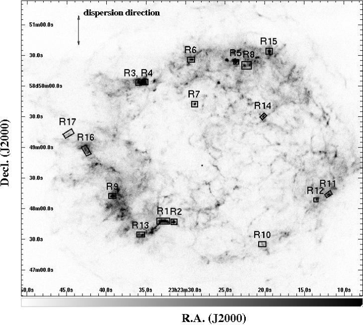
Figure 2: Zeroth-order Cas A image from this work. Regions used in the analysis of HETGS Cas A data. These regions are spatially narrow and they are isolated sufficiently above the local and extended background to provide a clear line profile for spectral fitting.

Figure 8: 3D Location and velocity of the regions. The line-of-sight velocity, as measured by Si lines and S lines, is plotted vs. the 2D projected distance on the sky from the nominal expansion center of Reed et al. (1995). The Si velocity values (diamonds) are given with 90% confidence error bars; the velocity values for S (stars) are given just for the best-fit value. An expansion rate of 0.19 % per year relates the velocity and distance scales (see text). The inner and outer solid lines indicate the locations of the reverse shock (95″) and the forward shock (153″) in year 2000 and centered on the Reed et al. (1995) velocity center (marked with triangle), ${\rm V_{center}}=+770$ km s^-1. Dotted lines at 102″ and 130″ are a guide to show the shell in which our regions generally lie. For reference, the location of the compact central object in Cas A (e.g. Chakrabarty et al., 2001) is also shown; its line-of-sight velocity is unknown.

Figure 10: Plot of plasma temperature $kT_{e}$ vs. ionization timescale $\tau=n_{e}t$ for 17 Cas A regions. The upper panel shows the full range of values, and the lower panel zooms in on the cluster of values. Three regions, R8, R10 and R17, show different properties from the rest. Region R6 is represented with two points, representing the mean value (lower left corner in the upper panel) and the upper limits (lower right corner in the upper panel).

Figure 11: The zeroth-order spectrum from region R9. The spectrum shows a good fit to the Mg, Si S, Ar and Ca lines and to the continuum part of the spectrum between 1.2 and 6 keV; Fe lines were not included in the fit and the part of the spectrum below 1.1 keV is not used in the fit.

Figure 12: The time-since-shocked in years is indicated for each region in a similar plot to Fig. 8. The red-shifted regions appear to have been shocked more recently compared to the regions on the front side which have longer $t_{\rm shock}$ values; the low Si XIV region, R6, with 0.5 yr is an exception.

Figure 14: Elevated continuum level in dispersed spectrum. The zeroth-order and MEG-first order spectra are shown for a simple MARX simulation of a monochromatic source embedded in a large region of continuum. The spectra are normalized to unit flux-in-the-line so that the equivalent widths, EW, of the lines serve as a measure of the continuum level. The EW for zeroth-order (left, dashed line) is 21.4 keV, whereas the dispersed spectrum has a reduced EW of 1.29 keV (right, dotted). Hence, relative to the line flux, the dispersed spectrum has an artificially higher continuum level due to overlapping continua from other locations along the dispersion axis.

References

- Anders & Grevesse (1989) Anders, E., & Grevesse, N. 1989, Geochimica et Cosmochimica Acta, 53, 197
- Becker et al. (1979) Becker, R. H., Smith, B. W., White, N. E., Holt, S. S., Boldt, E. A., Mushotzky, R. F., & Serlemitsos, P. J. 1979, ApJ, 234, L73
- Borkowski et al. (1996) Borkowski, K., Szymkowiak, A. E., Blondin, J. M., & Sarazin, C. L. 1996, ApJ, 466, 866
- Borkowski et al. (2001) Borkowski, K. J., Lyerly, W. J., & Reynolds, S. P. 2001, ApJ, 548, 820
- Bleeker et al. (2001) Bleeker, J. A. M., Willingale, R., van der Heyden, K., Dennerl, K., Kaastra, J. S., Aschenbach, B., & Vink, J. 2001, A&A, 365, L225
- Canizares et al. (2005) Canizares, C. R., et al. 2005, PASP, 117, 1144
- Chakrabarty et al. (2001) Chakrabarty, D., Pivovaroff, M. J., Hernquist, L. E., Heyl, J. S., & Narayan, R. 2001, ApJ, 548, 800
- Chevalier & Kirshner (1978) Chevalier, R. A., & Kirshner, R. P. 1978, ApJ, 219, 931
- Davis (2001) Davis, J. E., 2001, ApJ, 548, 1010.
- DeLaney & Rudnick (2003) DeLaney, T., & Rudnick, L. 2003, ApJ, 589, 818
- DeLaney et al. (2004) DeLaney, T., Rudnick, L., Fesen, R. A., Jones, T. W., Petre, R., & Morse, J. A. 2004, ApJ, 613, 343
- Dewey (2002) Dewey, D. 2002, High Resolution X-ray Spectroscopy with XMM-Newton and Chandra, Ed. Branduardi-Raymont, G., published electronically and stored on CD; http://www.mssl.ucl.ac.uk/g̃br/rgs_workshop/
- Fesen et al. (2006) Fesen, R. A., Hammell, M. C., Morse, J., Chevalier, R. A., Borkowski, K. J., Dopita, M. A., Gerardy, C. L., Lawrence, S. S., Raymond, J. C. & van den Bergh, S. 2006, ApJ, in press, (astro-ph/0603371)
- Fesen & Gunderson (1996) Fesen, R. A., & Gunderson, K. S. 1996, ApJ, 470, 967
- Fesen et al. (2001) Fesen, R. A., Morse, J. A., Chevalier, R. A., Borkowski, K. J., Gerardy, C. L., Lawrence, S. S., & van den Bergh, S. 2001, AJ, 122, 2644
- Flanagan et al. (2004) Flanagan, K. A., Canizares, C. R., Dewey, D., Houck, J. C., Fredericks, A. C., Schattenburg, M. L., Markert, T. H., & Davis, D. S. 2004, ApJ, 605, 230
- Gotthelf et al. (2001) Gotthelf, E. V., Koralesky, B., Rudnick, L., Jones, T. W., Hwang, U., & Petre, R. 2001, ApJ, 552, L39
- Holt et al. (1994) Holt, S. S., Gotthelf, E. V., Tsunemi, H., & Negoro, H. 1994, PASJ, 46, L151
- Houck (2002) Houck, J.C. 2002, High Resolution X-ray Spectroscopy with XMM-Newton and Chandra, Ed. Branduardi-Raymont, G., published electronically and stored on CD; http://www.mssl.ucl.ac.uk/g̃br/rgs_workshop/
- Hughes et al. (2000) Hughes, J. P., Rakowski, C. E., Burrows, D. N., & Slane, P. O. 2000, ApJ, 528, L109
- Hwang et al. (2000) Hwang, U., Holt, S. S., & Petre, R. 2000, ApJ, 537, L119
- Hwang et al. (2001) Hwang, U., Szymkowiak, A. E., Petre, R., & Holt, S. S. 2001, ApJ, 560, L175
- Hwang & Laming (2003) Hwang, U., & Laming, J. M. 2003, ApJ, 597, 362
- Hwang et al. (2004) Hwang, U., et al. 2004, ApJ, 615, L117
- Kamper & van den Bergh (1976) Kamper, K., & van den Bergh, S. 1976, PASP, 88, 587
- Laming & Hwang (2003) Laming, J. M., & Hwang, U. 2003, ApJ, 597, 347
- Lawrence et al. (1995) Lawrence, S. S., MacAlpine, G. M., Uomoto, A., Woodgate, B. E., Brown, L. W., Oliversen, R. J., Lowenthal, J. D., & Liu, C. 1995, AJ, 109, 2635
- Markert et al. (1983) Markert, T. H., Clark, G. W., Winkler, P. F., & Canizares, C. R. 1983, ApJ, 268, 134
- Mazzotta et al. (1998) Mazzotta, P., Mazzitelli, G., Colafrancesco, S., & Vittorio, N. 1998, A&AS, 133, 403
- Minkowski (1959) Minkowski, R. 1959, IAU Symp. 9: URSI Symp. 1: Paris Symposium on Radio Astronomy, 9, 315
- Paerels & Kahn (2003) Paerels, F. B. S., & Kahn, S. M. 2003, ARA&A, 41, 291
- Peimbert & van den Bergh (1971) Peimbert, M., & van den Bergh, S. 1971, ApJ, 167, 223
- Pepino et al. (2004) Pepino, R., Kharchenko, V., Dalgarno, A., & Lallement, R. 2004, ApJ, 617, 1347
- Porquet et al. (2001) Porquet, D., Mewe, R., Dubau, J., Raassen, A. J. J., & Kaastra, J. S. 2001, A&A, 376, 1113
- Pradhan (1982) Pradhan, A. K. 1982, ApJ, 263, 477
- Reed et al. (1995) Reed, J. E., Hester, J. J., Fabian, A. C., & Winkler, P. F. 1995, ApJ, 440, 706
- Stage et al. (2006) Stage, M. et al. 2006, in preparation
- Thorstensen et al. (2001) Thorstensen, J. R., Fesen, R. A., & van den Bergh, S. 2001, AJ, 122, 297
- Vink et al. (1996) Vink, J., Kaastra, J. S., & Bleeker, J. A. M. 1996, A&A, 307, L41
- Vink et al. (1998) Vink, J., Bloemen, H., Kaastra, J. S., & Bleeker, J. A. M. 1998, A&A, 339, 201
- Vink et al. (1999) Vink, J., Maccarone, M. C., Kaastra, J. S., Mineo, T., Bleeker, J. A. M., Preite-Martinez, A., & Bloemen, H. 1999, A&A, 344, 289
- Waldron & Cassinelli (2001) Waldron, W. L., & Cassinelli, J. P. 2001, ApJ, 548, L45
- Woosley et al. (1993) Woosley, S. E., Langer, N., & Weaver, T. A. 1993, ApJ, 411, 823
- Willingale et al. (2002) Willingale, R., Bleeker, J. A. M., van der Heyden, K. J., Kaastra, J. S., & Vink, J. 2002, A&A, 381, 1039
- Willingale et al. (2003) Willingale, R., Bleeker, J. A. M., van der Heyden, K. J., & Kaastra, J. S. 2003, A&A, 398, 1021