The Origin of the Bifurcation in the Sagittarius Stream

Abstract

The latest Sloan Digital Sky Survey data reveal a prominent bifurcation in the distribution of debris of the Sagittarius dwarf spheroidal (Sgr) beginning at a right ascension of $\alpha\approx 190^{\circ}$. Two branches of the stream (A and B) persist at roughly the same heliocentric distance over at least $50^{\circ}$ of arc. There is also evidence for a more distant structure (C) well behind the A branch. This paper provides the first explanation for the bifurcation. It is caused by the projection of the young leading (A) and old trailing (B) tidal arms of the Sgr, whilst the old leading arm (C) lies well behind A. This explanation is only possible if the halo is close to spherical, as the angular difference between the branches is a measure of the precession of the orbital plane.

1. Introduction

The disrupting Sagittarius dwarf spheroidal galaxy (Sgr) was discovered by Ibata, Gilmore & Irwin in 1994. It was soon realized that the Sgr provided a powerful tool for the study of the Galaxy (Ibata et al., 1997). The nucleus of the Sgr has survived for many orbits around the Galaxy, whilst its tidal tails have now been detected over a full $360^{\circ}$ on the Sky (see e.g. Totten & Irwin, 1998; Majewski et al., 2003; Belokurov et al., 2006). The disrupted fragments of the Sgr diffuse in the Galactic potential. As the pericenter of the Sgr’s orbit is $\sim 16$ kpc, whilst its apocenter is $\sim 60$ kpc, the debris provides a strong constraint on the Galaxy’s halo.

The morphology of the Sgr stream is known in detail in the Galactic southern hemisphere thanks to 2MASS (Majewski et al., 2003, 2004; Skrutskie et al., 2006). Newberg et al. (2002, 2003) made early detections of Sgr tidal debris in data from the Sloan Digital Sky Survey (SDSS, see Hogg et al., 2001; Stoughton et al., 2002; Smith et al., 2002; Pier et al., 2003; Ivezić et al., 2004; Gunn et al., 2006). Then, Belokurov et al. (2006) used a color cut to pick out the upper main sequence and turn-off stars in SDSS Data Release 5 (DR5, Adelman-McCarthy et al., 2006) belonging to the stream. In the Galactic northern hemisphere, they found a prominent bifurcation or branching in the stream, beginning at a right ascension $\alpha\approx 190^{\circ}$ (see the upper right panel of Figure 1). The lower and upper declination branches of the stream, labelled A and B, can be traced until right ascensions of at least $\alpha\approx 140^{\circ}$. Using the location of the subgiant branch as an estimator, the A and B branches are reckoned to be at similar distances. There is also evidence in the data of a fainter, still more distant stream (C) directly behind the A branch.

Belokurov et al.’s (2006) dataset is important for two reasons. First, it traces the Sgr stream around the North Galactic Cap, the very spot at which oblate and prolate dark halos give different predictions (e.g., Helmi, 2004a). Second, the debris in 2MASS is dynamically younger than that found in SDSS, so the SDSS data should give stronger constraints, as the stars have had longer to move in the Galactic potential.

Early explorations of the evolution of the Sgr suggested that the Galactic halo may be close to spherical (Ibata et al., 2001b; Majewski et al., 2003). For example, Johnston et al. (2005) showed that the precession apparent in Sgr debris in the 2MASS dataset strongly favored mildly oblate halos. However, Helmi (2004a) pointed out that many of the earlier datasets are restricted to stars that have only recently been torn off the Sgr and so have not diffused in the Galactic potential. In fact, Helmi (2004b) argued that the velocity measurements of 2MASS M giants in the leading arm favor strongly prolate halos and this was subsequently confirmed by Law et al. (2005). Hence, present studies of the disruption of the Sgr have reached an impasse, with different datasets pointing to dramatically different flattenings.

Here, our aim is to show how the newly discovered bifurcation arises. Using numerical simulations, we argue that the complex morphology of the Sgr stream uncovered by Belokurov et al. (2006) can only be reproduced if the Galaxy’s halo is close to spherical. Although our models do not resolve the contradiction between the precession rate and the velocities in the leading arm, they do provide a new and powerful argument in favor of an almost spherical Galaxy halo.

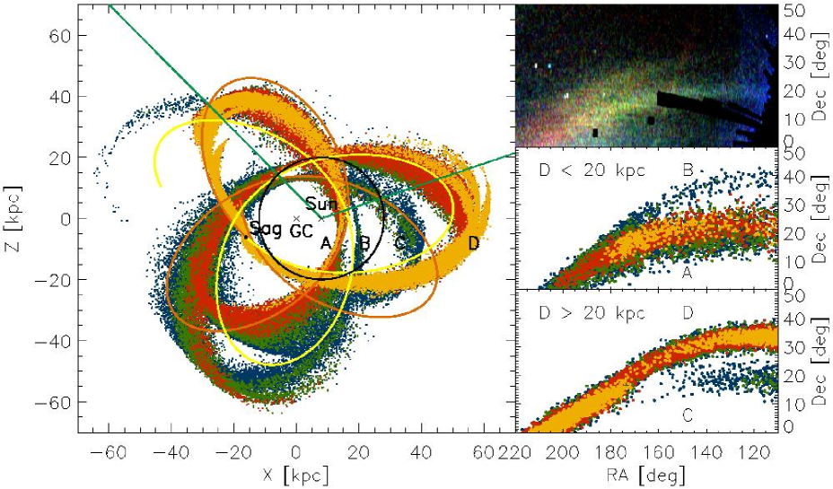
Figure 1.— Left: Simulation showing the tails of the Sgr dSph. Particles are color-coded according to when they were lost (gold: $<4$ Gyr ago, red: between $4$ and $5.7$ Gyr, green: between $5.7$ and $7.4$ Gyr and blue $>7.4$ Gyr ago). The yellow (orange) curves show the past (future) behavior of the Sgr’s orbit over 2 Gyr. The orbital period is 0.7 Gyr. The positions of the Galactic centre (GC), the Sun, and Sagittarius (Sag) are marked. The green lines show the right ascension range $110^{\circ}<\alpha<220^{\circ}$, which corresponds to the SDSS data analyzed by Belokurov et al. (2006). The 4 streams are marked A (young leading arm), B (old trailing arm), C (old leading arm) and D (young trailing arm). The circle gives the distance cut-off at 20 kpc. Upper Right: The SDSS data from Belokurov et al. (2006), with stars color-coded according to magnitude. Middle and Lower Right: Scatter plots in right ascension and declination of the tidal debris. Only particles within (beyond) a heliocentric distance of $20$ kpc are plotted in the middle (lower) panels. The black squares show the field locations of Belokurov et al. (2006). In the middle panel, streams A and B are clearly visible. The upper arm is the old trailing material, while the lower arm is the young leading material. In the lower panel, the old leading material is in the lower and the young trailing material in the upper branch. [The simulation uses a Miyamoto-Nagai disk and logarithmic halo with $q_{\phi}=1.05$, together with the set d of proper motions. The mass of Sgr is $10^{8}M_{\odot}$]

Table 1 Sets of proper motions used in the simulations.

Label	$\mu_{\alpha}\cos\delta$	$\mu_{\delta}$	$v_{\rm rad}$	Remarks
	(in mas yr-1)	(in mas yr-1)	(in km s-1)
a	-2.65	-0.88	137	HST measurement (Ibata et al 2001b)
b	-2.8	-1.4	137	Schmidt plates measurement (Irwin et al. 1996)
c	-2.9	-1.5	137	$<1\sigma$ variation of Schmidt plates
d	-3.02	-1.49	137	Simulation fit from Law et al. (2005)
e	-3.05	1.28	137	$5\sigma$ variation of HST values

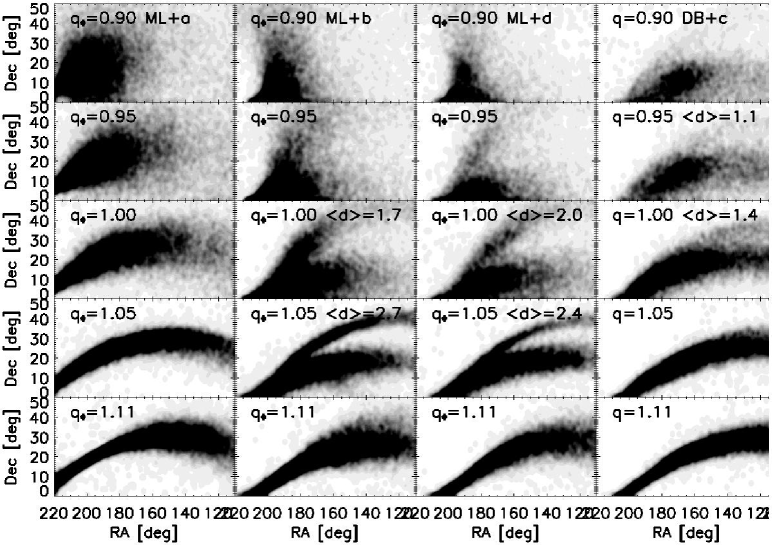
Figure 2.— The projected density of the young leading and old trailing tidal debris of the Sgr in a sequence of simulations with different halo flattenings, proper motions and Galaxy models. The key at the top of each column has the following significance: ML means Miyamoto-Nagai disk and logarithmic halo models, DB means the Dehnen & Binney models, whilst a, b, c, d or e refers to the choice of proper motions. The panels in a given column differ only in the flattening of the halo, with $q_{\phi}$ for the ML models and $q$ for the DB models recorded in the upper left corner. The mass of the Sgr is $10^{8}M_{\odot}$. Note that the particles in the simulation represent both stars and dark matter.

2. The Significance of the Bifurcation

The results of a typical simulation of the tidal disruption of the Sgr in a nearly spherical potential are shown in Fig. 1. We will give the details of the simulation set-up shortly, but at the moment our aim is to gain a qualitative understanding of why the bifurcation occurs. The particles in Fig. 1 are color-coded according to when they were torn off the Sgr. In the direction of the SDSS DR5 data – namely, the opening angle defined by the green lines – there are 4 distinct streams of material. They are the young leading arm (labelled A), the old trailing arm (B), the old leading arm (C) and the young trailing arm (D). Here, old and young indicate when the stars were torn off. 3 out of the 4 streams are identified in the SDSS DR5 dataset. Stars belonging to the D stream are more difficult to detect as they occur in DR5 primarily in the range $180^{\circ}\mathrel{\hbox to0.0pt{\lower 3.0pt\hbox{$\sim$}\hss}\raise 2.0pt\hbox{$<$}}\alpha\mathrel{\hbox to0.0pt{\lower 3.0pt\hbox{$\sim$}\hss}\raise 2.0pt\hbox{$<$}}220^{\circ}$, where they are not easy to untangle from the other streams. The simulation data are separated according to heliocentric distance and then projected onto the sky as viewed from the Sun, as shown in the lower right panels of Fig. 1. The young leading arm provides branch A and the old trailing arm branch B of the bifurcated stream of Belokurov et al. (2006). These two narrow branches are at similar heliocentric distances, as required to match the data. The material in these branches is about two revolutions apart in orbital phase. For the material beyond 20 kpc, the older leading material is in the lower declination branch, while the younger trailing material is in the upper. The old leading arm (C) provides the more distant and fainter stream detected by Belokurov et al. (2006) behind the A branch. The young trailing arm (D) lies behind the B branch and so is not the structure seen by Belokurov et al. (2006).

The Sun lies roughly in the orbital plane of the Sgr. If the potential were exactly spherical, the debris of the Sgr would lie in a single plane and no bifurcation would exist. Any asphericity (whether intrinsic to the halo or produced by the bulge and disk) causes the orbital plane to precess and therefore the planes of the 4 arms to be slightly different. The positional difference between branches A and B is a direct measure of the precession over two orbital revolutions and hence the asphericity of the potential. The facts that (i) branches A and B are so close in projection and (ii) branch C lies behind branch A suggest that the precession is small, and that the potential is close to spherical. If the halo is too oblate or prolate, then debris is scattered over a wide range of locations and does not lie in thin, almost overlapping streams on the sky. To back up this qualitative argument, let us now describe a suite of simulations developed to measure the properties of the bifurcation as a function of halo flattening, Sgr mass and proper motion.

Table 2 The Strength and Range of the Bifurcation in Nearly Spherical Haloes

Logarithmic Halo
$Q_{\phi}$	$q_{\phi}$	a	b	c	d	e
0.92	1.0	–	1.7	1.9	2.0	1.5
		–	$170^{\circ}$	$180^{\circ}$	$190^{\circ}$	$160^{\circ}$
0.95	1.05	–	2.7	2.3	2.4	1.7
		–	$190^{\circ}$	$190^{\circ}$	$170^{\circ}$	$150^{\circ}$

Dehnen & Binney Models
$Q_{\phi}$	$q$	a	b	c	d	e
0.95	0.95	–	1.1	1.1	–	–
		–	$160^{\circ}$	$150^{\circ}$	–	–
0.97	1.0	–	1.4	1.4	–	–
		–	$130^{\circ}$	$150^{\circ}$	–

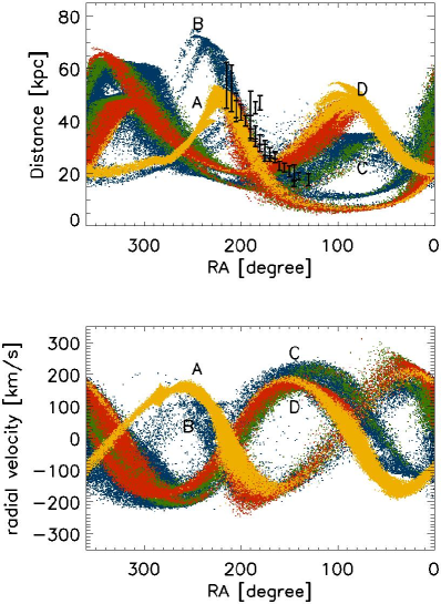
Figure 3.— Plots of the heliocentric distance and velocity versus right ascension for the same model as in Figure 1. Again, particles are color-coded according to when they were lost (gold: $<4$ Gyr ago, red: between $4$ and $5.7$ Gyr, green: between $5.7$ and $7.4$ Gyr and blue $>7.4$ Gyr ago). The datapoints give the heliocentric distances to the streams, as derived from fitting the subgiant branch described in Belokurov et al. (2006). Note that the distances to the A and B streams are too small for right ascensions $\alpha\mathrel{\hbox to0.0pt{\lower 3.0pt\hbox{$\sim$}\hss}\raise 2.0pt\hbox{$<$}}190^{\circ}$.

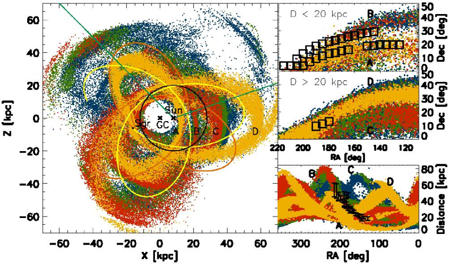
Figure 4.— As Figure 1, but now the mass of the Sgr has been increased to $5\times 10^{8}M_{\odot}$. A bifurcation is visible in the right-hand panels, but it is less dramatic than in the data.

3. Simulations

3.1. Set-up

The present position of the Sgr dSph is ($\alpha,\delta)=(283.7^{\circ},-30.5^{\circ}$), while its heliocentric distance is $25\pm 2$ kpc and radial velocity is $137\ {\rm kms}^{-1}$  (Ibata et al., 1997). Listed in Table 1 are two measurements of the proper motion of the Sgr, the first from Irwin et al. (1996) using Schmidt plates and the second from Ibata et al. (2001b) using HST data. Dinescu et al.’s (2005) recent measurement agrees with that of Irwin et al. (1996) within the errors. Given a choice of proper motions, we integrate back in time for $10$ Gyr adopting a potential for the Galaxy. At the final position, we insert a Plummer sphere containing $10^{6}$ particles with a scalelength of $350$ pc. We investigate models with a total mass of between $10^{8}$ and $10^{9}$ M_⊙. The particles are integrated forward using the particle-mesh N-Body code Superbox (Fellhauer et al., 2000) until the position today is reached again.

While the present position of the Sgr is unchanged in all our simulations, the range of proper motions recorded in Table 1 is investigated. For the Galactic potential, we use one of two possibilities. In the first (denoted by ML), the halo is represented by a logarithmic potential of the form

$$\Phi_{\rm halo}(r) = \frac{v_{0}^{2}}{2}\ln\left(R^{2}+z^{2}q_{\Phi}^{-2}+d^{2}\right),$$ (1)

with $v_{0}=186$ km s^-1 and $d=12$ kpc (where $R$ and $z$ are cylindrical coordinates). The parameter $q_{\Phi}$ is the axis ratio of the equipotentials. It controls whether the halo is spherical ($q_{\Phi}=1$), oblate ($q_{\Phi}<1$) or prolate ($q_{\Phi}>1$). In general, $q_{\Phi}$ is of course not the same as the axis ratio in the density $q$, which varies with radius for the logarithmic potential (see e.g., Evans 1993). The disc is represented by a Miyamoto-Nagai potential:

$$\Phi_{\rm disc}(R,z) = \frac{GM_{\rm d}}{\sqrt{R^{2}+\left(b+\sqrt{z^{2}+c^{2}}\right)^{2}}},$$ (2)

with $M_{\rm d}=10^{11}$ M_⊙, $b=6.5$ kpc and $c=0.26$ kpc. Finally, the bulge is modelled as a Hernquist potential

$$\Phi_{\rm bulge}(r) = \frac{GM_{\rm b}}{r+a},$$ (3)

using $M_{\rm b}=3.4\times 10^{10}$ M_⊙ and $a=0.7$ kpc. The superposition of these components gives quite a good representation of the Milky Way. The circular speed at the solar radius is $\sim 220$ km s^-1. The major advantage is the analytical accessibility of all quantities (forces, densities, and so on). Hence, this model has been very widely used – in particular, in many previous investigations of the Sgr stream (e.g. Helmi, 2004a, b; Johnston et al., 2005; Law et al., 2005).

In the second (denoted by DB), we use the Galactic potential suggested by Dehnen & Binney (1998). It consists of three disc components, namely the ISM, the thin and the thick disc, each of the form

$$\rho_{\rm disc}(R,z) = \frac{\Sigma_{\rm d}}{2z_{\rm d}}\exp\left(-\frac{R_{\rm m}}{R}-\frac{R}{R_{\rm d}}-\frac{|z|}{z_{\rm d}}\right).$$ (4)

With $R_{\rm m}=0$, equation (4) describes a standard double exponential disc with scale-length $R_{\rm d}$, scale-height $z_{\rm d}$ and central surface-density $\Sigma_{\rm d}$. For the stellar disks $R_{\rm m}$ is set to zero, while for the ISM disc, we allow for a central depression by setting $R_{\rm m}=4$ kpc. Furthermore, the halo and the bulge are represented by two spherical density distributions of the form

$$\rho_{\rm S}(R,z) = \rho_{0}\left(\frac{m}{r_{0}}\right)^{-\gamma}\left(1+\frac{m}{r_{0}}\right)^{\gamma-\beta}\exp\left(-\frac{m^{2}}{r_{\rm t}^{2}}\right),$$ (5)

where $m^{2}=R^{2}+z^{2}q^{-2}$ and $q$ is the axis ratio in the density. We choose the parameters according to the best-fit model 4 in Dehnen & Binney (1998). This provides a better representation of the Galaxy, but at somewhat greater computational cost.

3.2. Results

Snapshots of the distribution of tidal debris around the North Galactic Cap for some typical simulations are shown in Figure 2. We quickly see that most of the models do not look at all like the data. Only haloes close to spherical provide bifurcated streams. The simulated streams in moderately and strongly oblate or prolate haloes do not bifurcate.

To proceed further, we need to develop an objective criterion for identifying the bifurcation. We use a Marquand-Levenberg routine to fit a single Gaussian and two Gaussians to the declination distribution in the young leading and old trailing tidal debris. Models for which a single Gaussian is everywhere preferred (as judged by the $\Delta\chi^{2}$) are unacceptable, as they do not show two identifiable streams. If two Gaussians are a better fit than a single, then the ratio $d$ of the distance between the two peaks to the sum of the dispersions of each peak is computed as a function of right ascension. We refer to the mean value of this parameter, taken over all right ascensions $110^{\circ}\leq\alpha\leq 220^{\circ}$, as the strength of the bifurcation, $\langle d\rangle$. The onset of the bifurcation $\alpha_{0}$ is taken to be the right ascension when $d=1.5$. Applying this algorithm to Belokurov et al.’s (2006) dataset, the bifurcation has strength $\langle d\rangle\approx 1.7$ and begins at a right ascension $\alpha_{0}\approx 190^{\circ}$. For a range of simulations, the same quantities are recorded in Table 2. Both Galaxy models contain a flattened disk and bulge, so the model parameters ($q_{\phi}$ and $q$) are not a reliable guide to the overall flattening of the potential. Rather, we give in Table 2 the axis ratio of the equipotentials $Q_{\phi}$ at the mean of the pericentric and apocentric distances of the Sgr’s orbit.

There are a number of interesting conclusions from the Table. First, very few models actually give bifurcations at all. Of the 80 models tested, only 10 give bifurcated streams. A bifurcation occurs if the axis ratio of the potential $Q_{\phi}$ lies in the range $0.92\lesssim Q_{\phi}\lesssim 0.97$. The best overall match to the data is given by simulations using the Miyamoto-Nagai disk and logarithmic halo with $q_{\phi}=1$, together with sets c or d of proper motions. They reproduce the strength and the location of the bifurcation reasonably well. Second, if we use the proper motions measured by HST (set a, derived by Ibata et al., 2001b), we do not obtain bifurcated streams, whatever the halo flattening. The precession is controlled not just by the flattening of the potential, but also by the eccentricity of the orbit, and hence the proper motions. Sets b and c of proper motions, with values close to those derived from Schmidt plates (Irwin et al., 1996), provide much better fits. Third, Helmi (2004b) has claimed that strongly prolate haloes with $q\approx 1.65$ give the best fit to the 2MASS data on the right ascension, declination, heliocentric distance and radial velocity of the tidal debris. Such strongly prolate models do not match the bifurcated stream in the SDSS dataset. In fact, the claims of prolateness rely heavily on their choice of Galactic potential (Miyamoto-Nagai disk and logarithmic halo) and are not reproduced with the Dehnen & Binney models. The Miyamoto-Nagai disk declines like a power-law, rather than an exponential, and so it is reasonable to interpret the finding of prolateness or stretching of the halo as compensation for deficiencies in the disk model. Similarly, although some of the nominally prolate halo models ($q_{\phi}>1$) in Table 2 provide matches to the bifurcation data, the equipotentials are mildly oblate ($Q_{\phi}<1$) at the radii probed by Sgr’s orbit.

Nearly spherical models can reproduce the projected density of the Sgr stream around the Northern Galactic Cap. However, as is traditional in this area, our simulations do not fit all the data! For example, there is a mismatch of $\sim 20^{\circ}$ in the right ascension of the beginning of the C stream (c.f., the upper and lower right panels of Figure 1). Figure 3 shows the heliocentric distances and velocities of stream A and B for the simulation of Figure 1, together with the heliocentric distances derived by Belokurov et al. (2006) from subgiant branch fitting. The heliocentric distances of the simulated streams are within the observational error bars over the range of right ascensions $\alpha\gtrsim 190^{\circ}$, but they are too small for $\alpha\lesssim 190^{\circ}$. In common with other simulations in oblate haloes (see e.g., Johnston et al., 2005), the radial velocities of 2MASS M giants in the leading arm are also not matched. Possible causes of these discrepancies are discussed shortly.

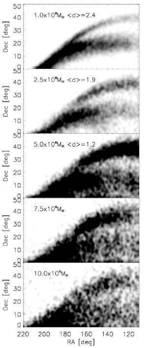
Figure 5.— A sequence of simulations differing only in the mass of the Sgr dSph at the beginning of our 10 Gyr simulations. This is marked in the top left-hand corner and varies from $2.5\times 10^{8}{{\rm M}_{\odot}}$ (top panel) to $10^{9}{{\rm M}_{\odot}}$ (bottom panel). If there is a bifurcation, then strength $\langle d\rangle$ is also recorded. The Galactic model is a Miyamoto-Nagai disk and logarithmic halo with $q_{\phi}=1.05$, while proper motion set d is used.

Table 3 Properties of the Models of the Sgr dSph.

Initial Mass	Final Mass	Final Velocity	Final Crossing
(in $10^{8}\,{{\rm M}_{\odot}}$)	(in $10^{8}\,{{\rm M}_{\odot}}$)	Dispersion (in km s-1)	Time (in Myr)
1.	0.5	19.	59
2.5	1.9	30.	38
5.	3.4	36.	46
7.5	5.7	44.	37
10	8.0	50.	32

The existence of the bifurcation also constrains the mass of the Sgr. For example, Figure 4 shows a simulation identical to that of Figure 1, but with the initial mass of the Sgr increased to $5\times 10^{8}M_{\odot}$. The more massive the Sgr, the greater its internal velocity dispersion. This has two consequences – the tidal arms are broader and they diffuse away from the Sgr’s orbital path more quickly. The overall effect is that debris is scattered over a wider range of locations. As the subpanels on the right hand side show, the bifurcation persists but is less dramatic than in the data, whilst the A and B streams are no longer as collimated as in the data. The run of heliocentric distances with right ascensions, however, is a somewhat better match. Figure 5 shows a sequence of simulations with Sgr masses between $10^{8}{{\rm M}_{\odot}}$ and $10^{9}{{\rm M}_{\odot}}$, while the Galactic potential is kept fixed as a Miyamoto-Nagai disk and logarithmic halo with $q_{\phi}=1.05$. The bifurcation blurs with increasing mass. Quantitively, the strength of the bifurcation $\langle d\rangle$ falls from 2.4 when the Sgr’s mass is $10^{8}{{\rm M}_{\odot}}$ to 1.9 at $2.5\times 10^{8}{{\rm M}_{\odot}}$ and to 1.2 at $5\times 10^{8}{{\rm M}_{\odot}}$. Once the Sgr mass rises much above $5\times 10^{8}{{\rm M}_{\odot}}$, there is no visible bifurcation. High mass models are disfavored until it has been demonstrated that the tidal streams of stars can remain as highly collimated as in the data. In Table 3, we give the properties of the Sgr remnant at the end of our simulations. Of course, our simulations show both dark matter particles and stars, whereas the observable today is the luminous matter left in the Sgr dSph. The mass loss of the Sgr is mainly affected by its orbit and hence the choice of proper motion together with the choice of Galactic potential. Since these are uncertain, we also give in Table 3 the internal crossing times at the virial radius and the three dimensional velocity dispersion, which governs the broadening of the tails.

Our overall picture gives three predictions. First, a second wrap of branch D may be detectable in the 2MASS data, closer than that already reported by Majewski et al. (2003). Secondly, the dynamically older B stream should have a larger velocity dispersion than the younger A stream. The mean velocities of branches A and B probably differ by $\sim 15$ kms^-1, though this may be hard to measure as it may be less than the stream’s internal dispersions. Thirdly, if our current ideas on the star formation history of the Sgr are correct (e.g., Grebel, 2000), then there may be a difference in the stellar populations of the streams. Stream A may contain evidence for a younger population that is not present in stream B.

4. Conclusions

The Sgr stream, as seen by the Sloan Digital Sky Survey (Belokurov et al. 2006), is composed of two branches (A and B) at about the same heliocentric distance visibly diverging at right ascensions $\alpha\approx 190^{\circ}$ to give a bifurcation, together with a third stream (C) aligned with the A branch, but well behind it. This complex and intricate morphology throws down an enormous challenge to modellers.

Here, we have given a physical picture of how this structure may arise. The bifurcation is caused by a projection of the young leading (A) and the old trailing (B) tidal arms of the Sgr, while the old leading arm (C) lies well behind A. The bifurcation between A and B, and the positioning of C behind A, can only be reproduced in simulations of the disruption of the Sgr if the halo is nearly spherical. Simulations in either moderately or strongly oblate or prolate haloes fail these tests by a wide margin. In particular, the bifurcation only exists if the axis ratio of the potential $Q_{\phi}$ at the radii sampled by the Sgr’s orbit lies in the range $0.92\lesssim Q_{\phi}\lesssim 0.97$. The physical explanation of this is easy to provide. The material in the A and B branches is about two revolutions apart in orbital phase. The angular difference on the sky between the A and B branches is therefore a direct measure of the precession of the orbital plane of the Sgr over two revolutions. As the angular difference is small, so the precession of the orbital plane is small, and so the potential muss to be close to spherical. If the potential is moderately prolate or oblate, debris is scattered over a much wider range of locations. The path from observation to theoretical conclusion is surprisingly direct and independent of detailed modelling.

The bifurcation also provides a strong constraint on the mass of the Sgr and its debris. If this is much larger than $5\times 10^{8}{{\rm M}_{\odot}}$, then the tidal streams are too diffuse to give a clear bifurcation. This also is easy to understand. As the internal velocity dispersion increases with progenitor mass, so the streams become broader and diffuse more quickly in the Galactic potential. The A and B branches do not then have the highly collimated appearance seen in the data.

Our simulations – like all other simulations of the disruption of the Sgr in the literature – do not agree with all the data. In particular, the detailed distances to the A, B and C streams given in Belokurov et al. (2006) are not reproduced over the full range of right ascension. Although this is a defect, the limitations of the commonly-used methodology for Sgr disruption simulations also need to be acknowledged. The underlying assumption is that the Galactic potential is static and unevolving over up to 10 Gyr timescales. This is clearly incorrect – the Milky Way is believed to have accreted $30\%$ of its mass over the last 5 Gyr (see e.g., van den Bosch, 2002; Neistein et al., 2006). Simulations typically show that the last major merger take place at about a redshift $z=1$, roughly 8 Gyrs ago (Navarro, Frenk & White, 1995). Although most of the mass will have accreted in the outer parts of the Galaxy, the Sgr’s orbit extends out to $\sim 60$ kpc and will surely been affected by this rearrangement. The formation of the Galactic bar has been dated to between 5 and 8 Gyr ago (see e.g., Sevenster, 1999a, b), and so bar-driven evolution of the inner Galaxy will also have caused substantial changes. The effects of time evolution are of much greater importance for the SDSS dataset than for the 2MASS dataset, which is restricted to dynamically younger material.

The strength of the argument presented in this paper is that it relies on the gross morphological features of the Sgr stream. To reproduce the detailed positions and velocities of stars in the A, B and C branches may well require a clearer understand of Galactic evolution. However, the existence of a bifurcation in nearly spherical potentials is a robust result. To challenge the main conclusion of this paper requires the devising of an alternative explanation of the existence of two streams that are closely matched in distance over a $\sim 50^{\circ}$ arc. In this respect, our argument compares favourably with other methods of determination of halo shape using methods such as the flaring of the neutral gas layer (e.g. Olling & Merrifield, 2000) or the stellar kinematics of halo stars (e.g., van der Marel, 1991). These are afflicted by systematic uncertainties regarding the contribution of the cosmic ray pressure or the orientation of the stellar velocity ellipsoid, for example. In contrast, the bifurcation in the Sgr stream is a clean, simple and direct test.

References

- Adelman-McCarthy et al. (2006) Adelman-McCarthy, J. K., et al. 2006, ApJS, 162, 38
- Belokurov et al. (2006) Belokurov V., et al. 2006, ApJ, 642, L37
- Dehnen & Binney (1998) Dehnen W., Binney J., 1998, MNRAS, 294, 429
- Dinescu et al. (2005) Dinescu D. I., Girard T. M., van Altena W. F., & López C. E. 2005, ApJ, 618, L25
- Evans (1993) Evans N.W., 1993, MNRAS, 260, 191
- Fellhauer et al. (2000) Fellhauer, M., Kroupa, P., Baumgardt, H., Bien, R., Boily, C.M., Spurzem, R., & Wassmer, N., 2000, New Ast., 5, 305
- Grebel (2000) Grebel, E. K. 2000, Bulletin of the American Astronomical Society, 32, 698
- Gunn et al. (2006) Gunn, J.E. et al. 2006, ApJ, in press
- Helmi (2004a) Helmi A. 2004a, MNRAS, 351, 643
- Helmi (2004b) Helmi A. 2004b, ApJ, 610, L97
- Hogg et al. (2001) Hogg, D.W., Finkbeiner, D.P., Schlegel, D.J., Gunn, J.E. 2001, AJ, 122, 2129
- Ibata et al. (1994) Ibata, R. A., Gilmore, G., & Irwin, M. J. 1994, Nature, 370, 194
- Ibata et al. (1997) Ibata R. A., Wyse R. F. G., Gilmore G., Irwin M. J., Suntzeff N. B. 1997, AJ, 113, 634
- Ibata et al. (2001a) Ibata R., Irwin M., Lewis G.F., & Stolte A. 2001a, ApJ, 547, 133L
- Ibata et al. (2001b) Ibata R., Lewis G.F., Irwin M., Totten E., & Quinn T. 2001b, ApJ, 551, 294
- Irwin et al. (1996) Irwin, M., Ibata, R., Gilmore, G., Wyse, R., & Suntzeff, N. 1996, ASP Conf. Ser. 92: Formation of the Galactic Halo…Inside and Out, 92, 84
- Ivezić et al. (2004) Ivezić, Ž. et al., AN, 325, 583
- Johnston et al. (2005) Johnston K.V., Law D.R., & Majewski S.R. 2005, ApJ, 619, 800
- Law et al. (2005) Law D.R., Johnston K.V., & Majewski S.R. 2005, ApJ, 619, 807
- Majewski et al. (2003) Majewski S.R., Skrutskie M.F., Weinberg M.D., & Ostheimer J.C. 2003, ApJ, 599, 1082
- Majewski et al. (2004) Majewski S.R., et al. 2004, AJ, 128, 245
- Navarro, Frenk & White (1995) Navarro J., Frenk C.S., White S.D.M., 1995, MNRAS, 275, 56
- Neistein et al. (2006) Neisetin E., van den Bosch F., Dekel A., 2006, MNRAS, in press (astro-ph/0605045)
- Newberg et al. (2002) Newberg H.J., et al. 2002, ApJ, 569, 245
- Newberg et al. (2003) Newberg H.J., et al. 2003, ApJ, 596, L191
- Olling & Merrifield (2000) Olling R.P., Merrifield M., 2000, MNRAS, 311, 361
- Pier et al. (2003) Pier, J.R., Munn, J.A., Hindsley, R.B, Hennessy, G.S., Kent, S.M., Lupton, R.H., Ivezic, Z. 2003, AJ, 125, 1559
- Sevenster (1999a) Sevenster M., 1999a, MNRAS, 310, 629
- Sevenster (1999b) Sevenster M., 1999b, ApSS, 265, 377
- Skrutskie et al. (2006) Skrutskie M.F., et al. 2006, AJ, 131, 1163
- Smith et al. (2002) Smith, J. A., et al. 2002, AJ, 123, 2121
- Stoughton et al. (2002) Stoughton, C. et al. 2002, AJ, 123, 485
- Totten & Irwin (1998) Totten, E. J., & Irwin, M. J. 1998, MNRAS, 294, 1
- van den Bosch (2002) van den Bosch, F., 2002, MNRAS, 331, 98
- van der Marel (1991) van der Marel, R. P. 1991, MNRAS, 248, 515