Swift observations of the 2006 outburst of the recurrent nova RS Ophiuchi:
I. Early X-ray emission from the shocked ejecta and red giant wind

Abstract

RS Ophiuchi began its latest outburst on 2006 February 12. Previous outbursts have indicated that high velocity ejecta interact with a pre-existing red giant wind, setting up shock systems analogous to those seen in Supernova Remnants. However, in the previous outburst in 1985, X-ray observations did not commence until $55$ days after the initial explosion. Here we report on Swift observations covering the first month of the 2006 outburst with the Burst Alert (BAT) and X-ray Telescope (XRT) instruments. RS Oph was clearly detected in the BAT 14-25 keV band from $t=0$ to $t\sim 6$ days. XRT observationsfrom 0.3-10 keV, started at 3.17 days after outburst. The rapidly evolving XRT spectra clearly show the presence of both line and continuum emission which can be fitted by thermal emission from hot gas whose characteristic temperature, overlying absorbing column, $[N_{H}]_{W}$, and resulting unabsorbed total flux decline monotonically after the first few days. Derived shock velocities are in good agreement with those found from observations at other wavelengths. Similarly, $[N_{H}]_{W}$ is in accord with that expected from the red giant wind ahead of the forward shock. We confirm the basic models of the 1985 outburst and conclude that standard Phase I remnant evolution terminated by $t\sim 10$ days and the remnant then rapidly evolved to display behaviour characteristic of Phase III. Around $t=26$ days however, a new, luminous and highly variable soft X-ray source began to appear whose origin will be explored in a subsequent paper.

1 Introduction

RS Ophiuchi (catalog ) is a Symbiotic Recurrent Nova (RN) which had previously undergone recorded outbursts in 1898, 1933, 1958, 1967 and 1985 (see Rosino, 1987; Rosino & Iijima, 1987), with a possible additional outburst in 1907 (Schaeffer, 2004). On 2006 February 12.83UT it was observed to be undergoing a further eruption (Hirosawa, 2006), reaching magnitude V=4.5 at this time. For the purposes of this paper, we define this as $t=t_{0}$. The optical light curve then continued a rapid decline, consistent with that seen in previous outbursts (Rosino (1987), AAVSO).

The RS Oph binary system comprises a red giant star in a $455.72\pm 0.83$ day orbit with a white dwarf (WD) of mass near the Chandrasekhar limit (see Dobrzycka & Kenyon, 1994; Shore et al., 1996; Fekel et al., 2000). Accretion of hydrogen-rich material from the red giant onto the WD surface leads to the conditions for a thermonuclear runaway (TNR) in a similar fashion to that for Classical Novae (CNe). The much shorter inter-outburst period for this type of RN compared to CNe is thought to be due to a combination of the high WD mass and a supposed high accretion rate (e.g. Starrfield et al., 1985; Yaron et al., 2005). Such models lead to the ejection of somewhat lower masses at higher velocities than those for CN models (typically 5000 km s^-1 and $10^{-8}-10^{-6}$M_⊙ respectively for RNe). Spectroscopy of RS Oph has indeed shown H$\alpha$ line emission with FWHM $=3930$ km s^-1 and FWZI $=7540$ km s^-1 on 2006 February 14.2 ($t=1.37$ days, Buil (2006)). Superimposed on the broad line is an intense and narrow double-peaked structure.

Unlike CNe, where the mass donor is a low-mass main-sequence star, the presence of the red giant in the RS Oph system means that the high velocity ejecta run into a dense circumstellar medium in the form of the red giant wind, setting up a shock system with gas temperatures $\sim 2.2\times 10^{8}$K for $v_{S}=4000$ km s^-1, where $v_{S}$ is the velocity of the forward shock running into the pre-existing wind (see below). Evidence for the presence of such high temperature material in outbursts prior to 1985 came from observations of coronal lines in optical spectra (Rosino, 1987) and the expected deceleration was evidenced by the narrowing of the initially broad emission lines (Snijders, 1987; Shore et al., 1996). The superimposed narrow lines are then from emission and absorption in the red giant wind ahead of the forward shock.

The interstellar absorbing column, $N_{H}=(2.4\pm 0.6)\times 10^{21}$ cm^-2, was determined from HI 21cm measurements (Hjellming et al., 1986) and is consistent with the visual extinction ($E(B-V)=0.7\pm 0.1$) determined from IUE observations in 1985 (Snijders, 1987). These quantities, together with the observed versus theoretical bolometric luminosity and apparent brightness of the red giant, are all consistent with a distance to RS Oph of $1.6\pm 0.3$ kpc (Bode, 1987).

EXOSAT observations in 1985 (Mason et al., 1987) from $t=55-251$ days post-outburst showed that RS Oph was initially an intense, then a rapidly declining soft X-ray source. Bode & Kahn (1985) formulated an analytical model of the evolution of the outburst based on the X-ray emission observed by EXOSAT at 55 days, the rapidly increasing radio emission from $t=18$ days (Padin et al., 1985) and parameters of the red giant wind derived from optical observations. They concluded that RS Oph evolved like a Supernova Remnant (SNR), but on timescales around $10^{5}$ times faster (see below). Subsequently, O’Brien & Kahn (1987) and O’Brien et al. (1992) constructed detailed analytical and numerical models of the interaction of the ejecta with the circumstellar medium which led to consistent estimates of the outburst energy and ejected mass of $1.1\times 10^{43}$ erg and $1.1\times 10^{-6}$ M_⊙ respectively, with the ratio of mass loss rate to outflow speed in the red giant wind being estimated as $6\times 10^{12}$ g cm^-1, compatible with that from isolated red giants. Perhaps not surprisingly, this relatively simple model failed to agree fully with the observed spectral evolution of the X-ray emission. In particular, it was difficult to reconcile both the low-energy and higher energy behaviour of the emission (see also Itoh & Hachisu (1990) who primarily explored the interaction of shells from two separate outbursts).

2 Swift Observations

Swift (Gehrels et al., 2004) is a multiwavelength mission primarily designed to detect gamma-ray bursts (GRBs). However the wide-field, hard X-ray Burst Alert Telescope (BAT, used for the detection of GRBs, Barthelmy et al. (2005)), and the X-ray telescope (XRT, used for their follow-up, Burrows et al. (2005)), are proving to be invaluable tools for sky monitoring and for observations of variable astrophysical objects such as novae.

2.1 BAT Observations

While awaiting GRBs, BAT normally operates in ‘survey mode’ in which spectral and imaging information is available with a time resolution which is typically 300s. A given part of the sky usually falls within the 1.4 sr BAT field of view many times per day. For example, 64 observations of RS Oph, totalling more than 9 hours, are available in the period 3 days either side of the optical detection of the outburst.

We have analysed all such data from $t=-20$ to +20 days using version 2.3 of the Swift software. Standard filtering was used to remove data affected by bad quality, high background rates, source occultations, etc. Two non-standard programs were used for the overlaying of images and for the extraction of source count rates while allowing for the presence of strong sources in the field of view. The latter allows for the intensity of all sources in the field of view to be fitted simultaneously, along with detector background models. It was used to calculate weighted means of the estimated intensity at the position of RS Oph in 4 broad bands (14-25, 25-50, 50-100 and 100-190 keV).

A clear detection of the source was made in the 14-25 keV band during the first 3 days from $t_{0}$ (Figure 1). In an overlay of images formed from the corresponding data, standard software (batcelldetect) finds a $9.9\sigma$ source within 2.5 arc minutes of the position of RS Oph as the only unidentified source above $5\sigma$, confirming the reality of this detection. There are tantalising hints of emission in this same band in the preceding few days, and also a weak detection in the 25-50 keV band immediately following the outburst, but these should be treated with caution and their evaluation awaits a more detailed analysis.

Standard software for spectral analysis was used. Spectra with 2 keV bins were extracted for each interval over which the pointing was unchanged (averaging 840 s). Systematic errors were taken into account and XSPEC Version 11.3.2 was used to fit models simultaneously to all the observations covering $\sim$1 day. The signal to noise ratio was never good enough to justify models with multiple free parameters and so only the normalisation was fitted.

Unfortunately, due to a BAT reboot, no data are available at the time of the first XRT observation discussed below, and when data again became available the source was comparatively weak. We have fitted the BAT 14-50 keV spectra with the simple spectral models found using the XRT data as detailed below. Satisfactory $\chi^{2}$ values were always found and allowing for the fact that BAT data are averages, and centered on slightly different times, the measured fluxes are consistent with extrapolations of the corresponding XRT spectra.

The RXTE All-sky Monitor observed the direction of RS Oph at several times during the period 2006 February 12-18 ($t\sim$0 to 5 days). Little or nothing is detected in band $a$ (1.3-3 keV) while in band $b$ (3-5 keV), and more particularly in band $c$ (5-12 keV), an increasing flux is seen. The fluxes are initially lower than expected from a model based on the first XRT observation, scaled to match the BAT data, but they reach the expected level by about February 15. This is consistent with an initially very high, but decreasing, absorption column. Sokoloski et al. (2006) have published an analysis of RXTE PCA observations starting from $t=3.1$ days The hard X-ray light curve implied by their results is consistent with Figure 1, although the BAT observations extend higher in energy and the XRT data described below provide better low energy coverage and energy resolution below 10 keV.

2.2 XRT Observations

Table 1 gives details of the Swift XRT observations carried out over the first 26 days following the outburst. These began at $t=3.17$ days (Bode et al., 2006; Bode, 2006) and continued at a frequency which has given excellent temporal coverage. This means that the observations began much earlier in the evolution of the outburst, and we were able to follow it in much more temporal and spectral detail, than was the case for the EXOSAT observations in 1985.

Swift software version 2.3 was used to process the data from the XRT. Source spectra were extracted from the cleaned Windowed Timing mode event-lists, using a box region of 60x20 pixels (1 pixel = 2.36 arcsec); the same region was then offset from the source to obtain a background spectrum. During some of the observations the source was positioned over the bad CCD columns (Abbey et al., 2006, caused by a micrometeorite impact on 2005-05-27) and we corrected for the fractional loss of the PSF incurred when calculating the count rate and flux.

Grade 0-2 events were chosen for the spectral analysis. The ftool xrtmkarf was used to generate suitable ancillary response function files and these were used in conjunction with the most up-to-date response matrix (swxwt0to2$\_$20010101v007.rmf).

All spectra were grouped to a minimum of 20 counts per bin in order to facilitate the use of the $\chi^{2}$ statistic in XSPEC, the results of which are discussed below. All fits included an energy scale offset that was allowed to vary between -0.1 and 0 keV to account for possible CCD bias measurement uncertanties. Errors are given at the 90 per cent level (e.g., $\Delta\chi^{2}$ = 2.7 for one degree of freedom).

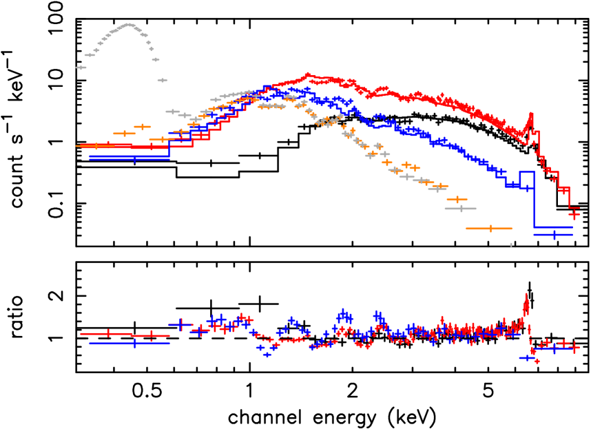
Figure 2: Selected Swift XRT spectra of RS Ophiuchi. Shown are data from $t=$ days 3.17 (black), 5.03 (red), 13.6 (blue), 25.99 (orange), and 29 (grey). The mekal, optically thin, collisionally-ionized plasma emission model fits shown are for days 3.17, 5.03 and 13.6, with their residuals plotted in the bottom panel.

Figure 2 shows a sample of the resulting spectra at selected epochs and Table 1 gives further information, including the results of the model fits described below. The initial count rate at $t=3.17$ days doubled in less than two days to peak at around 30 counts s^-1, then fell again until the emergence of a new soft component beginning at Observation 8 ($t=26$ days) which dominated the XRT spectrum by Observation 9 (Osborne et al., 2006a, $t=29$ days) - see Figure 2. The gross evolution of the spectrum was a progressive softening during the period of these X-ray observations.

3 Phases of Remnant Evolution

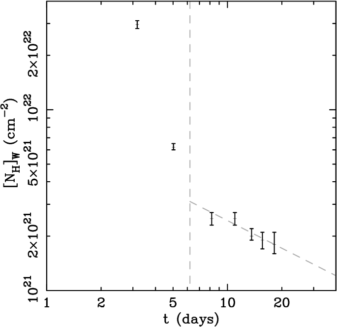
Figure 3: Temporal behaviour of the overlying absorbing column in the red giant wind, $[N_{H}]_{W}$, net of the assumed interstellar column of $2.4\times 10^{21}$ cm^-2, derived from the XRT spectral fits. A vertical dashed line on this Figure (and Figure 4) indicates the expected end of Phase I development. The diagonal dashed line is a power-law of index $\alpha=0.5$ . Note that Observation 8 is not shown as $[N_{H}]_{W}$ was fixed at the value derived for Observation 7 (see text for details).

In the earliest phase of the outburst, the ejecta from the WD surface are expected to traverse the binary system on a timescale $t\sim 2$d for $v_{ej}=3000$ km s^-1 (Dobrzycka & Kenyon, 1994; Fekel et al., 2000). Subsequent to this, using models previously applied to the evolution of SNR, Bode & Kahn (1985) found that Phase I (where the ejecta were still important in supplying energy to the shocked stellar wind) ended in the first few days after the 1985 outburst. Indeed, using the parameters derived by O’Brien et al. (1992) in Equations 5 and 9 of Bode & Kahn (1985), we derive $t\simeq 6.2$d for the duration of Phase I (see Figures 3 and 4). Thereafter, the remnant evolution can be well modelled by the instantaneous release of energy at a point. The Bode & Kahn (1985) analytical model of the 1985 outburst led to the conclusion that at the time the EXOSAT observations began ($t=55$d), the remnant was in the transition between Phase II (where a blast wave is being driven into the wind and is so hot as to be effectively adiabatic) and Phase III (where the shocked material is well cooled by radiation). Initially, a double shock system is established, with the forward shock being driven into the stellar wind and a reverse shock being driven into the otherwise unshocked ejecta. In Phase II, the Primakoff similarity solution for this type of explosion into an $r^{-2}$ density distribution (where $r$ is the radial distance from the site of the explosion) gives

$$r_{s}=at^{2/3}$$ (1)

where $r_{s}$ is the shock radius and $a$ is a parameter which is a function of the energy $E$ communicated by the ejecta to the shocked wind, the mass loss rate in the red giant wind $\dot{M}$ and the red giant wind velocity $u$. Similarly, in Phase III,

$$r_{s}=bt^{1/2}.$$ (2)

For a strong shock, the post-shock temperature $T_{s}$ is given by

$$T_{s}=\frac{3}{16}\frac{\bar{m}v_{s}^{2}}{k}$$ (3)

where $k$ is Boltzmann’s constant and $\bar{m}=10^{-24}$ g is the mean particle mass, including electrons.

The O’Brien et al. (1992) analytical models found good fits to the evolution of the remnant up to around $t=70$ days after outburst when there was a significant decline in soft X-ray flux. This was explored in terms of numerical models of the forward shock running off the end of the red giant wind re-established between the 1967 and 1985 outbursts, as suggested by Mason et al. (1987). However, O’Brien et al. (1992) noted that discrepancies between the observed X-ray and models, particularly evident at low energies, could be explained by a contribution from unveiling of the central nuclear burning source (see below). The final EXOSAT observation on day 251 was proposed as being consistent with low luminosity remnant nuclear burning on the WD surface (Mason et al., 1987).

4 Interpreting the Observations of the 2006 Outburst

In the 2006 outburst, the Swift XRT observations reported here started towards the end of the period in which Bode & Kahn (1985) concluded that the reverse shock running into the ejecta may still be important (Phase I), then cover the period of the expected Phase I/II transition and extend into that of Phase II/III.

From Table 1 and Figure 2 it can be seen that until around $t=26$ days (Observation 8) the observed X-ray flux at first rose rapidly, then gradually declined, becoming progressively softer with time. However, as noted above, an excess at energies below around 0.7 keV was evident from $t\sim 26$d onwards and this varied dramatically thereafter (Osborne et al., 2006b). A fuller exploration of the evolution of the soft component will be given in Osborne et al. (2006c).

Extensive model fitting of the early XRT results has been undertaken. The presence of obvious line emission, both in the XRT spectrum and from a higher resolution Chandra X-ray observation on 2006 February 26 (Ness et al., 2006), strongly suggested that models of emission from a high temperature thermal plasma were most appropriate. Our first order approach has therefore been to fit a single temperature mekal model to the emission using XSPEC, yielding both line and continuum radiation, with the thermal bremsstrahlung contribution being increasingly dominant at higher temperatures.

Up to and including Observation 7 at $t=18.17$ days, the fit was performed over the whole 0.3 - 10 keV range of the XRT data. After this date, only data for $E>$0.7 keV were used in order to separate out emission from the additional, highly variable, soft component seen after this time. We have constrained the interstellar column to be $[N_{H}]_{IS}=(2.4\pm 0.6)\times 10^{21}$ cm^-2 throughout (Hjellming et al., 1986) but we let the additional column from the overlying red giant wind, $[N_{H}]_{W}$, be a free parameter up to and including Observation 7. $[N_{H}]_{W}$ was then fixed at $1.8\times 10^{21}$ cm^-2 thereafter as the new soft X-ray emission component began to dominate the emission at low energies. Spectral fits at several epochs using a solar abundance model are shown in Figure 2. We note that elemental abundance enhancements were required by Bode & Kahn (1985) in their model and also by Snijders (1987) and (Shore et al., 1996) from IUE observations of the 1985 outburst. However, we choose solar abundances until we have performed detailed analyses of the evolution of the shell (as described further in the Discussion section below). We also note that these single temperature fits, as may be reasonably expected, fail to reproduce all of the spectral detail and should not be overly interpreted at this stage.

In the first three epochs, (Observations 1, 2a and 2b) the Fe K line was clearly detected at around 6.7 keV, as expected for the fitted plasma temperatures. In the first two epochs, there was also obvious excess emission at lower energies in the line compared to the single temperature mekal model fit. This could be characterised by an additional line at 6.4 keV which suggests X-ray reflection from a cold (or moderately ionised) gas as seen in some AGN and magnetic CVs (Beardmore et al., 1995; Done et al., 1995). We consider scattering in the red giant wind more likely in this case, a situation well documented in a number of supergiant X-ray binaries (e.g. van der Meer (2005) and references therein). The equivalent width of this line ($\sim 70$ eV in Observation 2a) is consistent with fluorescent emission by the surrounding gas with a column density $\sim 6\times 10^{22}$ cm^-2 (Makashima, 1985).

Figures 3 and 4 illustrate the results for important parameters derived from the fits. For example, Figure 3 shows a monotonic decline in $[N_{H}]_{W}$ with time, in a manner qualitatively expected as the forward shock traverses the overlying wind. The forward shock velocity, $v_{s}$, has been derived from the best fit plasma temperature and Equation 3 above. It can also immediately be seen that the implied shock velocities are of the same order as those derived spectroscopically (Buil, 2006; Evans et al., 2006; Ness et al., 2006). The unabsorbed X-ray flux, $F_{unabs}$, shows an initial rise to a peak at around $t=5$d (with $L_{X}\approx 1.2\times 10^{36}$ erg s^-1 between 0.3 and 10 keV at $d=1.6$ kpc) followed again by a subsequent decline.

We can also undertake a more quantitative exploration of the basic model from these results in combination with VLBA observations obtained on 2006 February 26 (O’Brien et al., 2006a, b). These were taken almost simultaneously with Observation 5 of Swift (day 13.6), and showed a clumpy ring of emission which, if associated with the forward shock, would give a radius of approximately $2.1\times 10^{14}$ cm at $d=1.6$ kpc. The value of $N_{H}$ in the overlying wind (the net neutral column derived from the fits and shown in Table 1 and Figure 3) can be found from

$$[N_{H}]_{W}=\frac{X}{4\pi m_{H}}\frac{\dot{M}}{u}[\frac{1}{r_{s}}-\frac{1}{r_{out}}]$$ (4)

where $X$ is the mass fraction of hydrogen in the wind, $m_{H}$ is the mass of a hydrogen atom, $u$ is the wind speed and $r_{out}$ is the outer wind radius ($=u\Delta t$, where $\Delta t$ is the time since the last outburst, $\sim 21.04$ years). With $X=0.7$ for solar composition, $u=20$ km s^-1 and $\dot{M}/u$ from O’Brien et al. (1992), this gives $[N_{H}]_{W}=9\times 10^{20}$ cm^-2, i.e. within a factor of two of the derived value from the single temperature model fits at this time (see Table 1). We note that $[N_{H}]_{W}$ derived in Equation 4 will be an underestimate for the value of the column for the whole shocked shell as it is calculated from the line-of-sight (front) edge. In addition, X-ray estimates of $[N_{H}]_{W}$ depend on the abundances in the wind (we have assumed these are solar) and furthermore Baumgartner & Mushotsky (2006) suggest that $[N_{H}]_{IS}$ derived from X-ray observations may differ somewhat from 21 cm values as it also samples H₂ in the ISM.

After $t\sim 6$ days, (by which time the Bode & Kahn (1985) model expected Phase I to be effectively over) it can be seen from Figure 4 that $v_{s}$ declines monotonically with time, following a power law decay from $t\sim 10$ days onwards. Here, $v_{s}\propto t^{-\alpha}$, where $\alpha\simeq 0.6$. This compares more precisely to the expected value of $0.5$ for Phase III, rather than $\alpha=0.33$, expected in Phase II evolution (Bode & Kahn, 1985). Equation 4 implies that $[N_{H}]_{W}\propto{t}^{-\alpha}$ at early times (as $r_{out}=1.3\times 10^{15}$ cm $\gg r_{s}$), where $\alpha=0.67$ (Phase II) or $0.5$ (Phase III) respectively. From Figure 3, it appears that after the implied end of Phase I, the data can in fact be better fitted by $\alpha=0.5$. Finally, after the expected end of Phase I, $F_{unabs}$ decayed as $t^{-1.5}$, as expected from a well-cooled shock.

The Sokoloski et al. (2006) observations of RS Oph with the RXTE PCA between days 3 and 21 are also consistent with the basic shock model. Their results imply Phase II evolution after the first few days from the behaviour of their derived temperature, but are more consistent with Phase III evolution during this period from the behaviour of the X-ray flux. The usable energy range of the PCA (2-25 keV) means however that their observations were less sensitive to $N_{H}$ and they did not detect the emergence of the soft component.

At $t=13.6$ days, our fits to the Swift data imply $v_{s}\simeq 1700$ km s^-1. We note that we could obtain complete consistency between the VLBA imagery and simple derivation of $v_{s}$ from the Swift model fits if $a=2.7\times 10^{10}$ cm s^-2/3 and a larger distance of $d=2.4$ kpc, if the remnant were behaving precisely as one would expect for the Primakoff (Phase II) solution throughout. However, the time dependence of $v_{s}$, $[N_{H}]_{W}$ and $F_{unabs}$ are more like what one would expect in Phase III, but in this case $b=3.7\times 10^{11}$ cm s^-1/2 and for consistency with the VLBA results, the distance would have to be increased to 3 kpc. Such high values of the distance were accepted prior to 1985 (Bode, 1987). On the other hand, Snijders (1987) notes that the failure to detect material at the typical velocities of the Carina Arm in IUE spectra places an upper limit on the distance to RS Oph of about 2 kpc. In addition of course, we have shown that there is a transition at around $t=6$ days between remnant phases. Thus although the simple analysis is supportive of the qualitative correctness of the current models, as outlined below, detailed physical modelling is required to build a fully self-consistent picture.

5 Conclusions and future work

Our X-ray observations of the very earliest phases of the 2006 outburst of RS Oph are broadly consistent with the basic model of remnant evolution proposed by Bode & Kahn (1985) and further explored by O’Brien et al. (1992). In particular, it appears that Phase I may have ended by $t\sim 6$d as predicted. However, our first-order analysis suggests that the remnant moved rapidly into Phase III in this outburst.

Fits to the XRT data have also been attempted using vmekal where the abundances have been allowed to vary. For the single temperature fit, this resulted in a trend of decreasing elemental abundance enhancement with time, as would be expected as emission from the enriched nova ejecta at early times becomes increasingly less significant than that from the generally less enriched red giant wind. A series of fits using multi-temperature mekals was also performed producing improved fits to the data. However, detailed models involving full hydrodynamical simulations are ultimately required to fit the X-ray data in a physically meaningful way. These simulations produce an evolving range of temperatures and densities with radius from the central source (see O’Brien et al. (1992)). Resonant scattering of X-rays in the red giant wind may also be occurring, and therefore some of the X-ray emission line flux may be due to photoionization of this gas by the X-ray emitting shock. In addition, VLBI results (O’Brien et al., 2006b) have shown that assumptions of spherical symmetry are called into question, and higher spatial dimension modelling may be required. We plan this more detailed modelling to be the subject of a future paper.

In future papers we will report the results of our continued monitoring of the source with Swift. As well as attempting to understand the origin of the highly variable soft X-ray component (to be discussed in Osborne et al. (2006c), and which may possibly arise from continued nuclear burning near the Eddington luminosity on the WD surface), we are particularly interested in detailed investigation of three subsequent predicted phases of development: (a) the epoch when the forward shock is forecast to reach the end of the red giant wind at around $t=80$ days, (b) the timescale for turn-off of the high luminosity phase of the TNR, and (c) the re-establishment of accretion in the central binary and the overlying wind from the giant.

Table 1: Summary of RS Oph XRT Observations and Spectral Fits.

Obs.	Date (Day)	Exposure	Count rate	kT	Correction	[NH]W	$\chi^{2}$/dof	Unabs. Flux
		(s)	(count s-1)	(keV)	Factor	(1022 cm-2)		(erg cm-2 s-1)
001	2006-02-16T00:05 (3.17)	664	14.2 $\pm$ 0.2	8.44${}^{+0.98}_{-0.91}$	1.2	2.96 $\pm$ 0.15	460/286	2.0 $\times$ 10-9
002a	2006-02-17T20:33 (5.03)	999	31.5 $\pm$ 0.2	8.54${}^{+0.50}_{-0.49}$	1.1	0.62${}^{+0.03}_{-0.02}$	993/585	2.7 $\times$ 10-9
002b	2006-02-21T00:10 (8.18)	844	19.8 $\pm$ 0.2	7.24${}^{+0.54}_{-0.39}$	1.0	0.25 $\pm$ 0.02	631/436	1.3 $\times$ 10-9
004	2006-02-23T19:37 (10.99)	950	15.5 $\pm$ 0.2	4.38 $\pm$ 0.23	1.3	0.25 $\pm$ 0.02	484/327	8.9 $\times$ 10-10
005	2006-02-26T10:18 (13.6)	897	12.3 $\pm$ 0.1	3.30 $\pm$ 0.15	1.1	0.20${}^{+0.02}_{-0.01}$	465/289	6.8 $\times$ 10-10
006	2006-02-28T10:31 (15.61)	1041	10.6 $\pm$ 0.1	2.83${}^{+0.10}_{-0.09}$	1.0	0.19 $\pm$ 0.02	559/283	4.9 $\times$ 10-10
007	2006-03-03T00:04 (18.17)	738	8.6 $\pm$ 0.1	2.36${}^{+0.11}_{-0.12}$	1.0	0.18${}^{+0.03}_{-0.02}$	353/206	3.6 $\times$ 10-10
008	2006-03-10T19:38 (25.99)	1605	6.5 $\pm$ 0.1	1.61${}^{+0.03}_{-0.02}$	1.1	0.18	708/189	2.5$\times$10-10

Figure 1: The flux from RS Oph in the bands 14-25 keV and 25-50 keV observed with Swift BAT. Units are ergs cm^-2 s^-1 and are based on count rates in these bands assuming the spectral form found from the observation 001 XRT data. The circles show the flux in the same energy bands from extrapolation of the models in Table 1. Means have been calculated over 24 h periods and are represented by a point at the weighted mean time, with horizontal error bars stretching from the first to the last sample included in the mean . The very irregular sampling leads to uneven horizontal error bars. The dotted line is the time of the first optical detection of the outburst.

Figure 4: The XRT-derived temporal behaviour of the shock velocity, $v_{s}$ (points with error bars) and unabsorbed (0.7 - 10 keV) flux, $F_{unabs}$ (crosses). The diagonal dashed lines are power-laws with index $\alpha=0.6$ (for $v_{s}$ points) and $\alpha=1.5$ (for $F_{unabs}$ - see text for details).

References

- Abbey et al. (2006) Abbey, A., et al., 2006, in “The X-ray Universe, 2005”, ESA-SP 604, p943
- Barthelmy et al. (2005) Barthelmy, S.D., Barbier, L.R., Cummings, J.R. , et al., 2005, Space Science Rev. 120, 143
- Baumgartner & Mushotsky (2006) Baumgartner & Mushotsky, 2006, ApJ, 639, 929
- Beardmore et al. (1995) Beardmore A.P., Done, C., Osborne, J.P.,& Ishida, M., 1995, MNRAS, 272, 749
- Bode (1987) Bode, M.F., 1987, in RS Ophiuchi (1985) and the Recurrent Nova Phenomenon, ed. M.F. Bode, Utrecht: VNU Science Press, p241
- Bode & Kahn (1985) Bode, M.F., & Kahn, F.D., 1985, MNRAS, 217, 205
- Bode et al. (2006) Bode, M.F., et al., 2006, IAUC, 8675
- Bode (2006) Bode, M.F., 2006, IAUC, 8677
- Buil (2006) Buil, C., 2006, CBAT 403
- Burrows et al. (2005) Burrows, D.N., et al., 2005, Space Science Reviews, 120, 165
- Dobrzycka & Kenyon (1994) Dobrzycka, D., & Kenyon, S.J., 1994, AJ, 108, 2239
- Done et al. (1995) Done, C., Osborne, J.P., & Beardmore, A.P., 1995, MNRAS, 276, 483
- Evans et al. (2006) Evans, A., et al., 2006, IAUC, 8682
- Fekel et al. (2000) Fekel, F.C., Joyce, R.R., Hinkle, K.H., &Skrutskie, M.F., 2000, AJ, 119, 1375
- Gehrels et al. (2004) Gehrels, N., et al., 2004, ApJ, 611, 1005
- Hirosawa (2006) Hirosawa, K., 2006, IAUC 8671
- Hjellming et al. (1986) Hjellming, R.J., van Gorkom, J.H., Taylor, A.R., Seaquist, E.R., Padin, S., Davis, R.J., & Bode, M.F., 1986, ApJ, 305, L71
- Itoh & Hachisu (1990) Itoh, H., & Hachisu, I., 1990, ApJ, 358, 551
- Makashima (1985) Makashima, K., 1985, in Physics of Accretion on to Compact Objects, eds K.O. Mason, M.G. Watson & N.E. White, Springer Verlag Berlin, p249
- Mason et al. (1987) Mason, K.O., Cordova, F.A., Bode, M.F., & Barr, P., in RS Ophiuchi (1985) and the Recurrent Nova Phenomenon, ed. M.F. Bode, Utrecht: VNU Science Press, p167
- Ness et al. (2006) Ness, J-U., et al., 2006, CBET, 415
- O’Brien & Kahn (1987) O’Brien, T.J., & Kahn, F.D., 1987, MNRAS, 228, 277
- O’Brien et al. (1992) O’Brien, T.J., Bode, M.F., & Kahn, F.D., 1992, MNRAS, 255, 683
- O’Brien et al. (2006a) O’Brien, T.J., Muxlow, T.W.B, Garrington, S.T., Davis, R.J., Porcas, R.W., Bode, M.F., Eyres, S.P.S., & Evans, A., 2006, IAUC 8688
- O’Brien et al. (2006b) O’Brien, T.J., et al., 2006, Nature, in press
- Osborne et al. (2006a) Osborne, J.P., et al., 2006a, ATel, 764
- Osborne et al. (2006b) Osborne, J.P., et al., 2006b, ATel, 770
- Osborne et al. (2006c) Osborne, J.P., et al. 2006c (in preparation)
- Padin et al. (1985) Padin, S., Davis, R.J., & Bode, M.F., Nature, 315, 306
- Rosino (1987) Rosino, L., 1987, in RS Ophiuchi (1985) and the Recurrent Nova Phenomenon, ed. M.F. Bode, Utrecht: VNU Science Press, p1
- Rosino & Iijima (1987) Rosino, L., & Iijima, T., 1987, in RS Ophiuchi (1985) and the Recurrent Nova Phenomenon, ed. M.F. Bode, Utrecht: VNU Science Press, p27
- Schaeffer (2004) Schaeffer, B., 2004, IAUC, 8396
- Shore et al. (1996) Shore, S.N., Kenyon, S.J., Starrfield, S., & Sonneborn, G., 1996, ApJ, 456, 717
- Snijders (1987) Snijders, M.A.J., 1987, in RS Ophiuchi (1985) and the Recurrent Nova Phenomenon, ed. M.F. Bode, Utrecht: VNU Science Press, p51
- Sokoloski et al. (2006) Sokoloski, J.L., Luna, G.J.M., Mukai, K., & Kenyon, S.J., 2006, Nature, in press
- Starrfield et al. (1985) Starrfield, S., Sparks, W.M., & Truran, J.W., 1985, ApJ, 291, 136
- van der Meer (2005) van der Meer, A., Kaper, L., di Salvo, T., Méndez, M., van der Klis, M, Barr, P. & Trams, N.R., 2005, A&A, 999, 1012
- Yaron et al. (2005) Yaron, O., Prialnik, D., Shara, M.M., & Kovetz, A., 2005, ApJ, 623, 398