Non-gaussianity for a Two Component Hybrid Model of Inflation

Abstract

We consider a two component hybrid inflation model, in which two fields drive inflation. Our results show that this model generates an observable non-gaussian contribution to the curvature spectrum, within the limits allowed by the recent WMAP year 3 data. We show that if one field has a mass $\eta_{\phi}<0$, and an initial value $\phi<0.06M_{\rm pl}$ while the other field has a mass $\eta_{\sigma}>0$, and initial field value $0.5M_{\rm pl}<\sigma\leq{}M_{\rm pl}$ then the non-gaussianity is observable with $1\lesssim f_{\rm NL}<1.5$, but that $f_{\rm NL}$ becomes much less than the observable limit should we take both masses to have the same sign, or if we loosened the constraints on the initial field values.

1 Introduction

We consider hybrid inflation driven by two scalar fields $\phi$ and $\sigma$, with the potential:

$$V=V_{0}\left(1+\frac{\eta_{\phi}}{2}\phi^{2}+\frac{\eta_{\sigma}}{2}\sigma^{2}\right)$$ (1)

where as usual the vacuum expectation value of the potential $V_{0}$ dominates, $\eta_{\phi},\eta_{\sigma}$ are the masses-squared of the $\phi$ and $\sigma$ fields respectively and may have either sign. We take $M_{\rm pl}=1$ throughout. This is similar to the case considered in Ref.[1, 2], with the $\sigma=0$ trajectory, and since the corresponding $|f_{\rm NL}|$ was found to be much less than $1$, we aim to derive the non-gaussianity generated by a more general trajectory. We calculate the curvature perturbation and the resulting non-gaussianity using the $\Delta{}N$ formalism [3] (which is equivalent to using second-order cosmological perturbation theory as described in [4]), for which:

$$\zeta(t,\textbf{x}) = \delta{}N$$ (2)

$$= N_{i}\delta\phi_{i}+\frac{1}{2}N_{ij}\delta\phi_{i}\delta\phi_{j}$$

Here $N$ is the unperturbed number of $e-$folds from an initial time with field values $\phi_{i}$ to a final time with energy density $\rho$, $N_{i}=\frac{\partial{}N}{\partial\phi_{i}}$ and $N_{ij}=\frac{\partial^{2}N}{\partial\phi_{i}d\phi_{j}}$ . We take the final time to be just before the end of inflation , and assume slow roll so that $\rho=V$.

We measure the non-gaussianity via the amplitude of the bi-spectrum:

$$\frac{3}{5}f_{\rm NL}=\frac{1}{2}\frac{N_{i}N_{ij}N_{j}}{\left(N_{n}N_{n}\right)^{2}}+4\ln(kaH)\mathcal{P}_{\zeta}\frac{N_{ij}N_{jk}N_{ki}}{\left(N_{m}N_{m}\right)^{3}}$$ (3)

where $\ln(kaH)\sim 1$, $k^{-1}$ is the scale under consideration, $a$ is the scale factor, $H=\dot{a}/a$ is the Hubble parameter, and $\mathcal{P}_{\zeta}$ is the spectrum of curvature perturbations. This expression assumes that the $\delta\phi_{i}$ are gaussian and applies even if $|f_{\rm NL}|\gtrsim{}1$ [6, 7], the condition for $f_{\rm NL}$ to eventually be observed.

2 The Derivatives

The amplitude of curvature perturbations defined in Eq. (2) is related to the amount of expansion that occurs between an initial time, corresponding to a flat slice of space-time and a final time, corresponding to a space time slice of uniform energy density. Following the procedure of [1] (which is equivalent to that used in Ref.[7]), the respective variations of the fields $\phi$ and $\sigma$ are defined purely by their initial values (denoted here as simply $\phi$ and $\sigma$) and the amount of inflation.

We use the slow roll equation:

$$3H\dot{\phi_{n}}+\frac{\partial{}V_{n}(\phi_{n})}{\partial\phi_{n}}=0$$ (4)

where $\dot{\phi_{n}}=d\phi_{n}/dt$. Rearranging this equation, and integrating over the period of inflation we get:

$$\int_{\phi_{n*}}^{\phi_{n}}\frac{d\phi_{n}}{\phi_{n}} = -\int_{t^{*}}^{t}\frac{\eta_{\phi}{}V_{0}}{3H}dt$$ (5)

$$= -\int_{0}^{N}\frac{\eta_{\phi}{}V_{0}}{3H^{2}}dN$$ (6)

where we have used $dN/dt\simeq{}H$ (valid for slow roll), and the $*$ denotes the time when cosmological scales left the horizon.

Recalling that $3H^{2}=\sum_{n}V(\phi_{n})\simeq{}V_{0}$ we have $\phi(N)=\phi\exp(-\eta_{\phi}{}N)$ and $\sigma(N)=\sigma\exp(-\eta_{\sigma}{}N)$. Substituting these equations into Eq. (1) we have:

$$V=V_{0}\left(1-\frac{\eta_{\phi}}{2}\phi^{2}\exp(-2\eta_{\phi}{}N)-\frac{\eta_{\sigma}}{2}\sigma^{2}\exp(-2\eta_{\sigma}{}N)\right)$$ (7)

differentiating Eq. (7) with respect to $\phi$, while recalling that $V_{i}=0$ and rearranging:

$$\frac{\partial{N}}{\partial\phi}=N_{\phi}=\frac{\eta_{\phi}\phi\exp(-2N\eta_{\phi})}{\beta}$$ (8)

where

$$\beta(\phi,\sigma,N)=\eta_{\phi}^{2}\phi^{2}\exp(-2N\eta_{\phi})+\eta_{\sigma}^{2}\sigma^{2}\exp(-2N\eta_{\sigma})$$ (9)

By differentiating Eq. (7) with respect to $\sigma$ we get:

$$N_{\sigma}=\frac{\eta_{\sigma}\sigma\exp(-2N\eta_{\sigma})}{\beta}$$ (10)

Defining:

$$\gamma(\phi,\sigma,N)=\eta_{\phi}^{3}\phi^{2}\exp(-2N\eta_{\phi})+\eta_{\sigma}^{3}\sigma^{2}\exp(-2N\eta_{\sigma})$$ (11)

we get:

$$N_{\phi\phi}=\frac{\eta_{\phi}\exp(-2N\eta_{\phi})}{\beta}-4\frac{\eta_{\phi}^{3}\phi^{2}\exp(-4N\eta_{\phi})}{\beta^{2}}+\frac{2\gamma}{\beta^{3}}\eta_{\phi}^{2}\phi^{2}\exp(-4N\eta_{\phi})$$ (12)

$$N_{\sigma\sigma}=\frac{\eta_{\sigma}\exp(-2N\eta_{\sigma})}{\beta}-4\frac{\eta_{\sigma}^{3}\sigma^{2}\exp(-4N\eta_{\sigma})}{\beta^{2}}+\frac{2\gamma}{\beta^{3}}\eta_{\sigma}^{2}\sigma^{2}\exp(-4N\eta_{\sigma})$$ (13)

and

$$N_{\phi\sigma}=N_{\sigma\phi}=\frac{2\eta_{\phi}\phi\eta_{\sigma}\sigma\exp(-2N(\eta_{\phi}+\eta_{\sigma}))}{\beta^{2}}\left(\frac{\gamma}{\beta}-(\eta_{\phi}+\eta_{\sigma})\right)$$ (14)

3 Curvature Perturbation

Substituting the equations from Section 2 into Eq. (2) we find that the curvature perturbation is given by the equation below. At first order, $\zeta$ is separable in terms of the individual field perturbations $\delta\phi$ and $\delta\sigma$, and involves a cross term $(\delta\phi\delta\sigma)$ at second order as well as the pure $(\delta\phi_{i})^{2}$.

$$\zeta = \frac{1}{2\beta}\Bigg{\{}2\eta_{\phi}\phi\exp(-2N\eta_{\phi})\delta\phi+2\eta_{\sigma}\sigma\exp(-2N\eta_{\sigma})\delta\sigma$$

$$+ \left[\eta_{\phi}\exp(-2N\eta_{\phi})-4\frac{\eta_{\phi}^{3}\phi^{3}}{\beta}\exp(-4N\eta_{\phi})+2\frac{\gamma}{\beta^{2}}\eta_{\phi}^{2}\phi^{2}\exp(-4N\eta_{\phi})\right](\delta\phi)^{2}$$

$$+ \left[\eta_{\sigma}\exp(2N\eta_{\sigma})-4\frac{\eta_{\sigma}^{3}\sigma^{3}}{\beta}\exp(-4N\eta_{\sigma})+2\frac{\gamma}{\beta^{2}}\eta_{\sigma}^{2}\sigma^{2}\exp(-4N\eta_{\sigma})\right](\delta\sigma)^{2}$$

$$+ 2\left[2\frac{\eta_{\phi}\phi\eta_{\sigma}\sigma\exp(-2N(\eta_{\sigma}+\eta_{\phi}))}{\beta}\left(\frac{\gamma}{\beta}-(\eta_{\phi}+\eta_{\sigma})\right)\right]\delta\phi\delta\sigma\Bigg{\}}$$

4 $f_{\rm NL}$

Substituting Eqs.(8) to (14) into Eq. (3) we find that the non-gaussian contribution to the curvature spectrum is given by:

$$\frac{3}{5}f_{\rm NL} = \frac{1}{2\left[\eta_{\phi}^{2}\phi^{2}\exp(-4N\eta_{\phi})+\eta_{\sigma}^{2}\sigma^{2}\exp(-4N\eta_{\sigma})\right]^{2}}$$ (16)

$$\times\Bigg{\{}-\beta\left[-\eta_{\sigma}^{3}\sigma^{2}\exp(-6N\eta_{\sigma})-\eta_{\phi}^{3}\phi^{2}\exp(-6N\eta_{\phi})\right]$$

$$+2\left[-2\eta_{\sigma}^{5}\sigma^{4}\exp(-8N\eta_{\sigma})-2\eta_{\phi}^{5}\phi^{4}\exp(-8N\eta_{\phi})\right.$$

$$\left.-2(\eta_{\phi}+\eta_{\sigma})\eta_{\phi}^{2}\eta_{\sigma}^{2}\phi^{2}\sigma^{2}\exp(-4N(\eta_{\sigma}+\eta_{\phi}))\right]$$

$$+2\frac{\gamma}{\beta}\left[\eta_{\sigma}^{4}\sigma^{4}\exp(-8N\eta_{\sigma})+\eta_{\phi}^{4}\phi^{4}\exp(-8N\eta_{\phi})\right.$$

$$\left.+2\eta_{\phi}^{2}\eta_{\sigma}^{2}\phi^{2}\sigma^{2}\exp(-4N(\eta_{\sigma}+\eta_{\phi}))\right]\Bigg{\}}+\cdots$$

We found that the second term is negligible with respect to the first, so we do not include it here.

5 The Positive-Negative Mass Combination

In this section we focus on taking $\eta_{\sigma}>0$ while $\eta_{\phi}<0$. In this case the $\sigma$ field is pushing the inflaton towards the origin while the $\phi$ field is pulling it away.

To first order in field perturbations, we find that the curvature perturbation Eq. (2) is dominated by the fluctuations in the negative mass field, since the fluctuations $\delta\sigma$ are exponentially damped.

$$\zeta=\frac{1}{\eta_{\phi}\phi}\delta\phi-\frac{2\eta_{\sigma}\sigma}{\eta_{\phi}^{2}\phi^{2}}\exp(2N(\eta_{\phi}-\eta_{\sigma}))\delta\sigma$$ (17)

This argument could be used to simplify the non-gaussian term (16) with only a small loss of precision, especially for the case where $\eta_{\sigma}\sim{}1$, and would reproduce the $f_{\rm NL}$ for a single field model. However this is not the case for $\eta_{\sigma}\ll{}1$, as then the exponent $2N\eta_{\sigma}\sim{}1$, and it becomes interesting to consider the affect of the $\delta\sigma$ fluctuations on observation.

6 The Spectral Index

For a multi-field inflaton the dominant term in the spectral index is defined by [8]:

$$n-1=2\frac{N_{a}N_{b}V_{ab}}{VN_{d}N_{d}}\\$$

so by substituting Eqs. (8) and (10), and using Eq. (1) to calculate $V_{ab}$ we get:

$$n-1=2\frac{\eta_{\phi}^{3}\phi^{2}\exp(-4N\eta_{\phi})+\eta_{\sigma}^{3}\sigma^{2}\exp(-4N\eta_{\sigma})}{\eta_{\phi}^{2}\phi^{2}\exp(-4N\eta_{\phi})+\eta_{\sigma}^{2}\sigma^{2}\exp(-4N\eta_{\sigma})}$$ (18)

From the recent WMAP year three data [9] the range of allowed $n-1$ for a negligible tensor fraction $r$ at the $2\sigma$ limit is:

$$-0.083<n-1<-0.02$$ (19)

If we want the spectral index to fall within observational limits regardless of initial conditions, then we require the spectral index given in Eq. (18) to fall within the observational bounds Eq. (19) independently of the initial field values. For the case where both $\eta_{\sigma},\eta_{\phi}<0$ then since Eq. (18) is a weighted sum of $2\eta_{i}$ we require:

$$|\eta_{i}|<0.041$$ (20)

However, for the case where $\eta_{\phi}<0$ and $\eta_{\sigma}>0$, then as long as $\eta_{\phi}$ satisfies the limits set by Eq. (20) then $\eta_{\sigma}$ can take on any value less than $1$, since for large values of $\eta_{\sigma}$ terms within the equations including it are exponentially damped. Also note that for positive field masses, $n-1>0$ which is ruled out by observation.

7 Results for the Non-Gaussianity

We begin by analyzing Eq. (16) for $N=50$. Keeping within the range of $\eta_{i}$ allowed by Eq. (19), we have analysed the potential for initial field values ranging between $(0-1)$, and values of the masses ranging between $(-0.04-0)$ for $\eta_{\phi}$ and $(-0.04-0.15)$ for $\eta_{\sigma}$. We then extracted the maximum value of $f_{\rm NL}$ for each combination of masses and plot the results in Fig1. We repeat this procedure and extract $|\frac{3}{5}f_{\rm NL}|_{max}$ for each combination of initial field values and plot these results in Fig2. We have also provided illustrations of the potential for the two scenarios considered in this paper in Figs3 and 4. For the case where $\eta_{\sigma}\to 0$ and $-0.04<\eta_{\phi}<0$, Eq. (16) reproduces the results for a single field scenario.

It is a far from easy task to extract any meaningful information from a four parameter model such as this one. However, both Figs. 1 and 2 are results of a full parameter space calculation of $f_{\rm NL}$, but Fig.1 shows the mass dependence of $|f_{\rm NL}|$, while Fig.2 shows the initial field value dependance of $|f_{\rm NL}|$ and by analyzing the figures we can see that for large $\sigma$, small $\phi$, and $\eta_{\sigma}>0,\eta_{\phi}<0$ we get $1\lesssim f_{\rm NL}<1.5$. Yet, if we were to consider small values of the fields $\phi,\sigma<0.1$, we see that $f_{\rm NL}\ll 1$ regardless of the values of the masses.

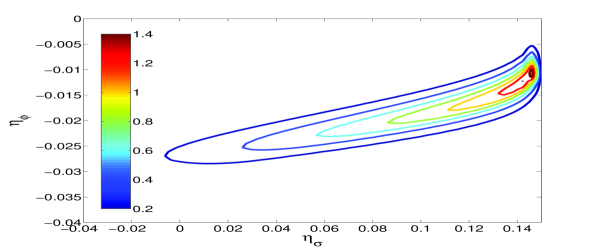
Figure 1: Contour plot of the absolute value of the maximum non-gaussianity generated for various combinations of masses, with initial conditions ranging between zero and the Planck mass. $|f_{\rm NL}|\gtrsim 1$ corresponds to the four inner contours and the region outside the outermost contour corresponds to $|\frac{3}{5}f_{\rm NL}|_{max}<0.2$.

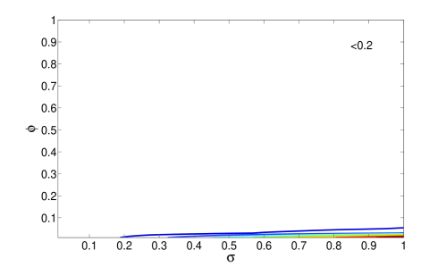
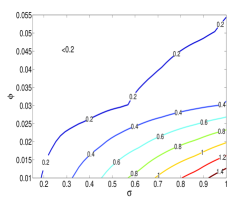
Figure 2: Contour plot of the absolute value of the maximum non-gaussianity generated for various combinations of initial field values, with masses $\eta_{\phi}$ ranging between ($-0.04-0$) and $\eta_{\sigma}$ ranging between ($-0.04-0.15$). The embedded plot is a magnification of the region in which $|\frac{3}{5}f_{\rm NL}|>0.2$ appears, note that this corresponds to $\phi\ll 1$ and $0.2\leq\sigma\leq 1$.

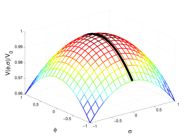
Figure 3: The potential Eq. (1) for $\eta_{\phi},\eta_{\sigma}>0$, in which the inflaton starts at a maximum and is pushed away from the origin by both fields. The solid black line corresponds to the unperturbed case $\sigma=0$

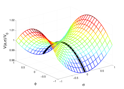
Figure 4: The potential Eq. (1) for $\eta_{\phi}>0$ and $\eta_{\sigma}<0$, in which the $\phi$ field pushes the inflaton away from the origin while the $\sigma$ field pulls it $towards$ it. This case produces the more significant (yet still undetectable) values of $f_{\rm NL}$ which appear in Figs.1&2. The solid black line corresponds to the unperturbed case $\sigma=0$

8 Discussion

We summarise the main results in the table below, and by Consistent with $n-1$? we mean does it satisfy the limits on the spectral index in Eq. (19).

					Consistent
$\eta_{\sigma}$	$\eta_{\phi}$	$\sigma$	$\phi$	$|f_{\rm NL}|$	with
					$n-1$?
$0<\eta_{\sigma}\ll 1$	$<0$	$<1$	$\ll 1$	$1\lesssim|f_{\rm NL}|<1.5$	yes
$<1$	$<0$	any value	any value	single field case	yes
				$|f_{\rm NL}|\ll 1$
$<0$	$<0$	any value	any value	$|f_{\rm NL}|\ll 1$	yes
any value	any value	$\ll 1$	$\ll 1$	$|f_{\rm NL}|\ll 1$	yes
$>0$	$>0$	any value	any value	not	no
				calculated	$n-1>0$
$\to 0$	$<0$	any value	any value	single field case	yes
				$|f_{\rm NL}|\ll 1$

For the first result listed $\eta_{\sigma}\ll 1$, considering that an unperturbed trajectory corresponds to $\sigma=0$ (solid black lines in Figs 3 and 4), the non-gaussian contribution to the curvature spectrum is due to the slight deviation in the inflaton trajectory caused by the $\sigma$ field, and since $-2N\eta_{\sigma}\sim 1$, the effect ‘survives’ inflation, leaving it’s imprint on the spectrum. In the $\eta_{\sigma}<1$ case, the roll to the minimum occurs rapidly at the beginning of inflation (by rapidly we mean on a time scale much smaller than the time scale of inflation), and thus the effect is negligible, and the results for the non-gaussianity are equivalent to a single field case $\frac{3}{5}f_{\rm NL}\simeq\eta_{\phi}/2$.

It is only fair to point out that we have not provided a physical motivation for this type of model with field values of order one, and since much effort was put into justifying multi-field chaotic models (as summarized in [10]), it is not clear whether we can write down our potential without justification.

9 Acknowledgements

I thank David H. Lyth and Karim Malik for helpful suggestions. I also thank Lancaster University for the award of the studentship from the Dowager Countess Eleanor Peel Trust.

References

- [1] D. H. Lyth and Y. Rodriguez, “The inflationary prediction for primordial non-gaussianity,” Phys. Rev. Lett. 95 (2005) 121302 [arXiv:astro-ph/0504045].
- [2] I. Zaballa, Y. Rodriguez and D. H. Lyth, “Higher order contributions to the primordial non-gaussianity,” JCAP 0606 (2006) 013 [arXiv:astro-ph/0603534].
- [3] M. Sasaki and E. D. Stewart, “A General analytic formula for the spectral index of the density perturbations produced during inflation,” Prog. Theor. Phys. 95 (1996) 71 [arXiv:astro-ph/9507001]. D. H. Lyth, K. A. Malik and M. Sasaki, “A general proof of the conservation of the curvature perturbation,” JCAP 0505, 004 (2005) [arXiv:astro-ph/0411220].
- [4] K. A. Malik and D. Wands, “Evolution of second order cosmological perturbations,” Class. Quant. Grav. 21, L65 (2004) [arXiv:astro-ph/0307055].
- [5] D. H. Lyth, “Generating the curvature perturbation at the end of inflation,” JCAP 0511, 006 (2005) [arXiv:astro-ph/0510443]. L. Alabidi and D. Lyth, “Curvature perturbation from symmetry breaking the end of inflation,” arXiv:astro-ph/0604569. M. P. Salem, “On the generation of density perturbations at the end of inflation,” Phys. Rev. D 72, 123516 (2005) [arXiv:astro-ph/0511146].
- [6] D. H. Lyth and I. Zaballa, “A Bound Concerning Primordial Non-Gaussianity,” JCAP 0510, 005 (2005) [arXiv:astro-ph/0507608].
- [7] F. Vernizzi and D. Wands, “Non-Gaussianities in two-field inflation,” JCAP 0605, 019 (2006) [arXiv:astro-ph/0603799].
- [8] A. R. Liddle and D. H. Lyth, “Cosmological Inflation and Large Scale Structure”, (CUP, Cambridge, 2000)
- [9] D. N. Spergel et al., “Wilkinson Microwave Anisotropy Probe (WMAP) three year results: Implications for cosmology,” arXiv:astro-ph/0603449.
- [10] L. Alabidi and D. H. Lyth, “Inflation models and observation,” JCAP 0605, 016 (2006) [arXiv:astro-ph/0510441].