The FSVS Cluster Catalogue: Galaxy Clusters and Groups in the Faint Sky Variability Survey

Abstract

We describe a large sample of 598 galaxy clusters and rich groups discovered in the data of the Faint Sky Variability Survey. The clusters have been identified using a fully automated, semi-parametric technique based on a maximum likelihood approach applied to Voronoi tessellation, and enhanced by colour discrimination. The sample covers a wide range of richness, has a density of $\sim 28$ clusters deg^-2, and spans a range of estimated redshifts of $0.05<z<0.9$ with mean $\langle z\rangle=0.345$. Assuming the presence of a cluster red sequence, the uncertainty of the estimated cluster redshifts is assessed to be $\sigma\sim 0.03$. Containing over 100 clusters with $z>0.6$, the catalogue contributes substantially to the current total of optically-selected, intermediate-redshift clusters, and complements the existing, usually X-ray selected, samples. The FSVS fields are accessible for observation throughout the whole year, making them particularly suited for large follow-up programmes. The construction of this FSVS Cluster Catalogue completes a fundamental component of our continuing programmes to investigate the environments of quasars and the chemical evolution of galaxies. We publish here the list of all clusters with their basic parameters, and discuss some illustrative examples in more detail. The full FSVS Cluster Catalogue, together with images and lists of member galaxies etc., will be issued as part of the “NOAO data products”, and accessible at http://www.noao.edu/dpp/. We describe the format of these data and access to them.

1 Introduction

Galaxy clusters are important for the study of structure formation and evolution, and their distribution provides important constraints on cosmological models. The number density of rich galaxy clusters is sensitive not only to the comoving distance measure but also to the rate of growth of fluctuations and hence the matter density $\Omega_{m}$. The low matter density models predict larger fluctuations at earlier times, because the growth of structure ceases earlier. Using the Press-Schechter formalism [Press & Schechter 1974] this predicts more clusters of a given mass at high redshift. However, large uncertainties arise when using cluster surveys to constrain cosmological parameters due to systematic uncertainties in the modelling of cluster formation and evolution [Viana & Liddle 1999]. Any progress in this field depends strongly on the availability of large cluster samples covering a wide parameter space, which require a multiplicity of selection methods. This justifies the large effort being invested into detection of these largest gravitationally bound systems by probing different regions of the electromagnetic spectrum.

Following the analysis of the first-year WMAP data the cosmological model can be studied with very high detail (Spergel et al. 2003) and combining the WMAP data with that of large surveys of galaxies (e.g. 2dF and SDSS), the cosmological parameters can be constrained with high precision (Hawkins et al. 2003, Percival et al. 2002). Nevertheless, the cosmological model remains undecided in the sense that the cause of the accelerated expansion is unknown. Parker, Komp & Vanzella (2003), for example, point out the power of counts of clusters (or galaxies) as a function of redshift to address this fundamental issue.

Abell (1958) constructed the first cluster catalogue by a systematic approach to the visual inspection of photographic plates. Zwicky et al. (1961–1968) constructed another large catalogue, also using visual inspection. Improvement of the performance and accessibility of computers allowed the implementation of fully automated cluster algorithms (e.g. Shectman 1985, Dodd & MacGillivray 1986). Since spectroscopic information is limited to very small areas of sky or to low redshifts (e.g $z\sim 0.15$ for the 2dFGRS, Colless et al. 2001), the challenge for cluster detection algorithms is to reduce the projection effects using only photometric data. Postman et al. (1996) introduced a matched filter (MF) algorithm — a maximum-likelihood method, which assumes a filter for both the cluster radial profile and the luminosity function of the cluster galaxies. At the same time as improvements to the original MF resulted in the adaptive matched filter (AMF, Kepner et al. 1999), many other statistical and astronomical concepts found applications in galaxy cluster surveys. Voronoi tessellation (VT) has been applied very successfully in connection with thresholding of the density peaks (Ramella et al. 2001, Söchting, Clowes & Campusano 2002, Kim et al. 2000), and recently improved by incorporating a maximum likelihood estimator (MLE, Söchting, Clowes & Campusano 2004) and colour discrimination (Kim et al. 2002). Colour discrimination is based on the fact that members of all known galaxy clusters trace a narrow sequence in colour-magnitude — the cluster red sequence (CRS) —, which was first proposed by Gladders & Yee (2000) as a means to increase the contrast of galaxy clusters above background galaxies.

We have used the images and object catalogues from the Faint Sky Variability Survey (FSVS, Groot et al. 2003) to identify galaxy clusters and groups and hence create the FSVS Cluster Catalogue. (Note that our application, being very different from that for which the FSVS was created, is one example of the usefulness of the “Virtual Observatory.”) The primary motivations for finding galaxy clusters in the FSVS data are the study of: (i) the galaxy environments favouring the formation of quasars, and hence the main mechanisms of formation as a function of redshift; and (ii) the chemical evolution of galaxies and dependences on environment. We chose VT, enhanced by MLE and a colour-cut, to construct a morphologically-unbiased sample (Okabe et al. 2000, Allard & Fraley 1997), containing structures with a wide range of richnesses and evolutionary stages. The resulting cluster catalogue, containing $\sim 600$ groups and clusters at $0.05<z<0.9$, complements the existing samples which at intermediate redshifts are usually biased towards X-ray luminous and/or optically very rich clusters.

We describe the data from the FSVS in Section 2 and the cluster detection technique in Section 3. In Section 4 we present the properties of the FSVS Cluster Catalogue. Section 5 contains the basic tabular data for all FSVS clusters and describes briefly the on-line access to the complete catalogue data.

2 Data

The FSVS provides a unique combination of spatial coverage and depth in three optical passbands with very high photometric and astrometric accuracy. The survey used the 2.5 metre Isaac Newton Telescope (INT) on La Palma to cover, in $B$, $V$ and $I$, 79 fields of moderate to high galactic latitude sky (see Table 1), totalling $\sim 23$ deg². The limiting magnitudes are $B\sim 24.5$ mag., $V\sim 25$ mag., and $I\sim 24$ mag. The completeness reaches a peak at $B\sim 24.0$ mag., $V\sim 23.5$ mag., and $I\sim 21.5$ mag. (Figure 1). Owing to poor quality, four fields (nos. 7, 36, 51, 67) have been excluded from this investigation, leading to a final coverage of $21.75$ deg². For more information on the FSVS data products see Groot et al. (2003) and Huber (2002). The photometry database for the FSVS is currently available for on-line access at http://www.astro.uva.nl/$\sim$fsvs/.

Table 1: The approximate positions of the FSVS fields (RA, Dec and $l^{II}$, $b^{II}$) and contiguous areas occupied by field groupings. (From Huber 2002.)

Field No.	RA	Dec	$l^{II}$	$b^{II}$	area
	(J2000)	(J2000)	[deg]	[deg]	[deg2]
1–6	23:44	$+$27:15	105	$-$33	1.74
8–12	02:32	$+$15:00	156	$-$40	1.45
13–18	07:52	$+$20:40	200	$+$22	1.74
19–22	12:53	$+$27:01	220	$+$90	1.16
23–26	12:51	$+$26:20	268–360	$+$89	1.16
27–30	16:25	$+$26:33	45	$+$43	1.16
31–34	17:20	$+$27:00	49	$+$31	1.16
35, 37–40	03:02	$+$18:38	161	$-$33	1.45
41–46, 59	07:15	$+$21:00	196	$+$15	2.03
47–50, 60	10:00	$+$21:30	211	$+$50	1.45
52–56	16:23	$+$27:03	45	$+$42	1.45
57–58	16:32	$+$21:16	39	$+$39	0.58
61–62	10:37	$+$04:00	242	$+$50	0.58
63–66	17:25	$+$27:30	50	$+$30	1.16
68–71	22:02	$+$27:30	83	$-$21	1.16
72–75	18:32	$+$36:00	64	$+$19	1.16
76–79	23:47	$+$28:10	106	$-$32	1.16

Figure 1: The magnitude distribution of the FSVS data in $B$ (top), $V$ (middle) and $I$ (bottom) using Field 3 as an illustrative example. All objects, point-like and extended, have been included.

2.1 Star-Galaxy Separation

Star-galaxy separation is carried out using the parameter stellarity, from the source detection program SExtractor [Bertin & Arnouts 1996]. It is based on the extended nature of the identified source and can have values ranging from 0 to 1, with 1 corresponding to a point-source. In Figure 2 we have plotted the stellarity as a function of magnitude for $V$ data, which, benefiting from the variability sampling, has improved the signal-to-noise ratio using co-added multiple field pointings. The quality does vary from field to field, which is best illustrated by comparison of the best (Field 22), in terms of the depth, resolution and galactic latitude, and worst (Field 65) fields in the top and bottom plots of Figure 2.

Figure 2: The stellarity as a function of magnitude in $V$. To illustrate the variation of the quality of co-added $V$ frames, the best frame (Field 22), (in terms of the depth, resolution and galactic latitude), average frame (Field 03), and worst frame (Field 65) have been shown.

There is no obvious cutoff between point and extended sources but the empirical data from follow-up spectroscopy and matching to the SIMBAD/VizieR database supports the threshold of 0.8. It provides the best separation (Huber 2002) between stars (stellarity $\geq 0.8$) and galaxies (stellarity $<0.8$) to a high magnitude ($V\sim 22.0$). As shown in Figure 3, within the range of 0.75 to 0.85, the exact value of the threshold stellarity has little impact on the object selection. The number of selected galaxy-like objects varies by $<1\%$ in most of the fields and $<3\%$ in fields with data of lowest quality. Beyond these limits, however, the number of selected galaxy-like objects start to change more rapidly (depending also on the data quality for a given field) and may influence the contrast of galaxy structures above the background and consequently their detection rate. The redder objects (which are important for our study) appear to be much less sensitive to the choice of the stellarity threshold than bluer objects.

Figure 3: The impact of the threshold stellarity on the object selection. The increment of galaxy-like objects selected for stellarity values of 0.70, 0.75, 0.8, 0.85 and 0.90 (upper dotted, upper solid, dashed, lower solid and lower dotted lines respectively) is expressed in percent relative to the number of objects selected for stellarity value of 0.8. The effect is plotted as a function of the colour of the colour-magnitude filter (the CM filter will be described in detail later in this paper). To illustrate the variation of the quality of co-added $V$ frames, the best frame (top, Field 22) and worst one (bottom, Field 65) have been shown.

2.2 Stellar Contamination

At the faint end of the data ($V>22.0$), the star-galaxy separation is increasingly unreliable and more and more stars are classified as extended objects. The relative contamination by stars at $V>22.0$ among faint extended sources is expected to vary as a function of the galactic latitude owing to variation of the typical star counts. It can also vary from field to field owing to enhanced numbers of galaxies where rich clusters occur. For these reasons the contamination by stars at $V>22.0$ has been estimated for every field separately. Using the magnitude distribution of point and extended sources at $V\leq 22.0$ the relative contribution of point and extended sources has been determined as a function of magnitude. Figure 4 gives the magnitude distributions of all sources, point sources, and extended sources using Fields 18, 61 and 21, with galactic latitudes $+22^{\circ}$, $+50^{\circ}$, and $+90^{\circ}$, as illustrative examples. The distributions at $22.0<V<25.0$ are extrapolated from exponential fits of the point-source and extended distributions for $V\leq 22.0$, then scaled, for $V>22.0$, according to the overall numbers of detected objects. The distributions show an obvious dependence of the stellar contamination on the galactic latitude. However, even at the lowest latitudes, galaxies substantially outnumber stars at the faint limits of the data ($V>22.0$). Under the assumption that the star population at such faint magnitudes will comprise only a minority of the objects and that their spatial distributions are fairly uniform compared with those of the galaxies (see Jones et al. 1991 for the variance of star and galaxy counts), all faint objects satisfying stellarity $<0.8$ have been included in the master database for identifying galaxy clusters.

Figure 4: The distributions with magnitude of the point and extended sources, and their extrapolated values for $V>22.0$, using Fields 18, 61 and 21 as illustrative examples. These fields have, respectively, $b^{II}=+22^{\circ}$, $b^{II}=+50^{\circ}$ and $b^{II}=+90^{\circ}$. The stellar contamination is decreasing with increasing galactic latitude. The distribution of all objects is denoted by the solid line, extended sources by the dashed line, and point-like sources by the dotted line. The vertical dotted line indicates the $V=22.0$ transition point to extrapolated values.

3 Method

Our main concern in the selection of clusters was the avoidance, as far as possible, of selection bias by using non-parametric methods to minimise the assumptions about the properties of the clusters. Söchting et al. (2004) proposed Voronoi tessellation (VT) enhanced by a maximum likelihood estimator (MLE) to better delineate the boundaries of the clusters, plus colour discrimination to reduce the contamination from background galaxies. The use of colour information provides the additional bonus of relatively accurate cluster redshifts deduced from the cluster red sequence (CRS, Gladders & Yee 2000).

The technique has been described in detail by Söchting et al. (2004), but with application to SuperCosmos $B_{J}-R$ data, which, of course, is intrinsically different from FSVS data. The SuperCosmos data cover the whole of the southern sky using shallow ($B_{J}<23$ and $R<21.5$) photographic plates whereas the FSVS data cover a relatively small area with deep ($B<24.5$, $V<25$ and $I<24$) CCD exposures. The $B_{J},~{}R$ SuperCosmos data allow us to probe the redshift range $z<0.3$ across wide areas of sky, whereas the FSVS Cluster Catalogue can reach $z\sim 1$ but only across relatively small fields. Consequently, the low redshift ($z<0.3$) galaxy clusters and superclusters are best detected using the SuperCosmos Sky Survey (or, for example, the Sloan Digital Sky Survey in the north) whereas the FSVS data are best suited to finding galaxy clusters at intermediate redshift ($0.3<z<1$) and poor groups at $z<0.3$.

These differences demand enhancements beyond the Söchting et al. (2004) method, focusing on using colour discrimination to improve the contrast enhancement over the large range of redshifts covered by the FSVS data. The Monte Carlo test of the detection rate (including completness and false detections) published in Söchting et al. (2004) as a function of contrast are independent of colour and remain fully valid for the FSVS data.

3.1 Voronoi Tessellation Technique

VT provides a partition of the investigated area into convex cells around every galaxy (Figure 5). The inverse of the area of a Voronoi cell gives the number density at the position of the galaxy. Since only the spatial structure of the galaxy distribution decides the sizes of the cells, VT provides a non-parametric method of sampling the underlying density distribution.

Figure 5: Example of Voronoi tessellation constructed on a uniformly distributed point set (from Söchting et al. 2003). For more information on Voronoi tessellation see Okabe et al. (2000) and references therein.

Galaxy clusters are detected as peaks in the galaxy density ($\delta$) distribution. The simplest approach to locate the density peaks is to select objects that exceed a threshold $\sigma$ for the density contrast with respect to the background. The density contrast $\sigma_{i}$ at the position of the $i$th object is defined as

$$\sigma_{i}=(\delta_{i}-\bar{\delta})/\bar{\delta},$$ (1)

where $\delta_{i}$ is the density and $\bar{\delta}$ is the mean density. One should remember that using Voronoi cells the mean density is calculated as

$$\bar{\delta}=\frac{1}{n}\sum_{i=1}^{n}\frac{1}{A_{i}}$$ (2)

where $A_{i}$ is the area of the Voronoi cell around object $i$ and $n$ is the overall number of objects. Until now this approach has been applied in all VT-based procedures, producing good results [Ramella et al. 2001, Kim et al. 2002, Söchting, Clowes & Campusano 2002]. Thresholding, however, introduces a bias towards clusters in regions of enhanced background, because it is not locally adaptive. Söchting et al. (2004) proposed an enhancement to this approach through a maximum likelihood estimator (MLE). Following the mathematical framework proposed by Allard & Fraley (1997), the log-partial-maximised-likelihood of a set of galaxies to be a cluster can be expressed as

$$l(\mn@boldsymbol{x};{\mathcal{A}})=-n\ln{n}+N_{A}\ln{\frac{N_{A}}{|A|}}+(n-N_{A})\ln{\frac{n-N_{A}}{1-|A|}}.$$ (3)

where $|A|$ denotes the normalised area of the cluster (the physical area of the cluster $\mathcal{A}$ divided by the physical area of a FSVS field $K$) and $N_{A}$ is the number of cluster member galaxies. By constructing $\mathcal{A}$ from Voronoi cells we ensure that any spatial constraints are defined by the data points themselves.

Without advance knowledge of the number and approximate positions of clusters in the data set, the MLE is very computationally intensive, losing the speed advantage of the basic VT. To accelerate the computation, the thresholding is preserved, but as a preliminary step (to produce a candidate list for the MLE algorithm), and MLE is used in the main process to reduce false detections (spurious clusters) and find the member galaxies in the confirmed clusters. The application of the MLE allows us to choose a rather low threshold, ensuring that the poor clusters in the regions of lower background density will be included. If the density of the cluster galaxies is $\delta_{cl}$ and that of the background galaxies $\bar{\delta_{b}}$ then the contrast is

$$\sigma=\frac{(\delta_{cl}+\bar{\delta_{b}})-\bar{\delta_{b}}}{\bar{\delta_{b}}}=\frac{\delta_{cl}}{\bar{\delta_{b}}}.$$ (4)

Since $\delta_{cl}=N_{A}/\mathcal{A}$ and $\bar{\delta_{b}}=(n-N_{A})/K$ this becomes

$$\sigma=\frac{N_{A}}{\mathcal{A}}\frac{K}{n-N_{A}}.$$ (5)

Then, since ${\mathcal{A}}/K=|A|$, the contrast of a cluster is

$$\sigma=\frac{1}{n-N_{A}}\frac{N_{A}}{|A|}$$ (6)

Assuming that the overall number of objects in the sample is very high compared with the number of cluster members, the size of an average Voronoi cell in a cluster is approximately

$$\langle|A_{cl}|\rangle\approx\frac{1}{n\sigma}$$ (7)

Using synthetic clusters, Söchting et al. (2004) have determined that the best performance is achieved by a threshold of $\sigma=2.0$ (i.e. all cells satisfying $A_{i}\leq 1/(2.0~{}n)$ are selected), achieving a detection rate of the synthetic clusters close to $100\%$ with contamination by spurious clusters less than $30\%$ of the overall number of clusters detected.

To suppress chance associations, groups with fewer than seven members present in the final cluster sample (after applying MLE) have to be discarded. The minimum number of members has been dictated by basic statistical properties of Voronoi tessellation. Assuming a Poisson distribution, the mean number of vertices/edges of a typical cell is 6 (Okabe et al. 2000), marking the natural threshold for random associations. Poor galaxy groups, which are all affected by this constraint, will be addressed in future work, using a somewhat different technique.

3.2 Colour Discrimination

The cluster detection rate and the contamination by spurious clusters depend strongly on the contrast of clusters above background, which can be increased by applying a colour discrimination. The use of colour slices was proposed and tested by Gladders & Yee (2000). The colour-magnitude slices used by Söchting et al. (2004) with $B_{J}$ and $R$ data have proved appropriate for detecting galaxy clusters at low redshifts ($z<0.3$), where the slopes and zero-points of the CRS are well known. At higher redshifts, the majority of the known galaxy clusters have been discovered by X-rays, and only a few of them have well-studied photometric properties. Beyond $z\sim 0.5$ the theoretically predicted parameters of the CRS are highly dependent on the selected models [Kodama et al. 1998], and would introduce a strong bias if incorporated in an algorithm for detecting clusters. The wide range of redshifts expected to be covered with FSVS data requires the introduction of a broader colour-magnitude filter to accommodate the strong variation of the parameters of the CRS. The shape of the filter must accommodate: (1) at low redshift ($z<0.3$) the population of faint cluster galaxies, for which the colour distribution is broader than that of the bright cluster spheroids; (2) at higher redshift ($z>0.3$), where only the bright cluster galaxies are detected, the uncertainty in the slope of the CRS. Figure 6 illustrates the shape of the filter we have adopted.

Figure 6: Example of a colour-magnitude filter (the polygon) used to enhance the contrast of galaxy clusters in the FSVS data. Asterisks denote galaxies that are identified as cluster members — they are within both the cluster boundary and the colour-magnitude filter; pluses denote galaxies within the cluster boundary but outside the colour-magnitude filter.

The filter is narrow at the bright end of the $I$ axis and gradually widens towards bluer colours at the faint end, enclosing a locus known from the galaxy distribution in low $z$ clusters. The purpose of the filter is to maximize, at any given redshift, the contrast of a galaxy cluster above the background, sometimes at the expense of some cluster galaxies staying outside the selection (e.g. the brightest members of the richest clusters at $z<0.2$, or a large fraction of the blue late-type galaxies). By moving the filter up the colour axis in $\Delta(V-I)=0.05$ steps, higher redshifts are probed. The filter is not moved along the luminosity axis ($I$), contrary to any expected allowance for galaxies becoming fainter with increasing redshift. Instead, the position of the filter remains unchanged with respect to the $I$ axis, allowing the bright galaxies of the higher redshift clusters to fall within the wider region of the filter, which accommodates a wide range of CRS slopes.

3.3 The Cluster Detection Algorithm

The MLE procedure to find galaxy clusters has been applied to every FSVS field separately. No attempts have been made to apply it across the boundaries of adjacent fields because of potential difficulties if the depths are different. In most cases, clusters that cross boundaries will be recognised and united in the later stages when multiple detections are consolidated.

The detection algorithm consists of the following steps. (1) Select all objects for which ($V-I$) and $I$ satisfy the criteria of the first colour filter. (2) Calculate the Voronoi tessellation for this selection. (3) Find which Voronoi cells satisfy $A_{i}\leq 1/(2.0~{}n)$. These are the cluster candidates. Multiple adjacent cells satisfying the criterion are treated as one candidate. (4) Apply the MLE to every candidate cluster. If the candidate consists of multiple cells then start with the smallest cell. (5) Move the colour filter by $\Delta(V-I)=0.05$ and repeat steps 1–4 until the whole colour space is covered. (6) Combine clusters that share the majority of the members. (7) For every cluster, place the colour filter to cover the CRS marked by its members. Select all objects within this filter and the cluster boundary (defined as the smallest convex hole enclosing all Voronoi tessells of the members) as the final cluster members. (8) Discard clusters with fewer than seven members.

The above procedure is sensitive to clusters that are truncated by the field boundary if at least seven cluster galaxies have Voronoi cells with edges that do not intersect the field boundary. In contrast, those methods that match a pre-defined radial profile are ineffective. Clusters detected at the field boundaries are flagged in the on-line catalogue, since some of their parameters (e.g. richness and radius) reflect only the fraction of the cluster contained by the FSVS field.

3.4 Calibration of Cluster Redshifts

The redshifts of the clusters can be estimated empirically, using the colour of the CRS, if some of the clusters have known spectroscopic redshifts. Ideally, the spectroscopic redshifts should cover the whole redshift range accessible by the survey. However, only four galaxy clusters with published spectroscopic redshifts were originally covered by the FSVS data, which would provide only a restricted calibration sequence. To construct a continuous sequence, redshifts of five additional clusters were obtained through the service programme at the Wiliam Herschel Telescope using the ISIS instrument. Data reduction was performed using standard IRAF routines. The combined sample used for redshift calibration is listed in Table 2.

Table 2: FSVS clusters with spectroscopic redshifts used for the redshift calibration of the cluster colours. The spectroscopic redshifts originate from the following sources: (1) Mullis et al. 2003; (2) Popesso et al. 2004; (3) Novicki, Sornig & Henry 2002; and (4) WHT ISIS service observations.

Cluster ID	$z$	$C_{cl}$ [$V-I$ mag]	Ref.
FSVS$\_$CL163105$+$212141	0.098	1.48	1
FSVS$\_$CL172015$+$263858	0.161	1.40	2
FSVS$\_$CL172030$+$274013	0.164	1.62	2
FSVS$\_$CL023057$+$144500	0.36	2.11	4
FSVS$\_$CL162339$+$263433	0.427	2.13	3
FSVS$\_$CL220532$+$270715	0.50	2.35	4
FSVS$\_$CL172531$+$274247	0.56	2.56	4
FSVS$\_$CL071535$+$212351	0.81	2.89	4
FSVS$\_$CL234150$+$265516	0.93	3.15	4

The second challenge is to find appropriate point of reference within the colour distribution of the cluster members which would allow robust colour-to-redshift association independent of cluster richness. At low redshift, often the zero-point of the CRS or the colour at a fixed magnitude along the CRS was selected as such a point of reference. However, the slopes of the CRS vary as a function of redshift and also as a function of richness [Söchting 2002], plus the uncertainty in the measurement of the slope increases with redshift because of the limited range of available magnitudes. For these reasons we use the colour $C_{fl}$ of the colour-magnitude filter (defined as the maximum colour covered by the filter) in which a cluster has been detected instead of the zero-point of the CRS. For the majority of the rich clusters both values agree very closely.

Figure 7: The redshift calibration curve. “Cluster colour” refers to the colour of the colour-magnitude filter (defined by its horizontal upper limit) in which the cluster has been detected. It is also the maximum colour allowed for a member galaxy. Triangles indicate nine calibration points (FSVS clusters with spectroscopic redshifts) including corresponding error bars. To provide an independent test of the calibration sequence, 13 galaxy clusters with published $VI$ magnitudes (Stanford et al. 2002) and spectroscopic redshifts have been included (asterisks). Dotted, dashed and dot-dashed lines indicate $1\sigma$, $2\sigma$ and $3\sigma$ limits respectively.

The resulting calibration function for a polynomial fit to spectroscopic redshifts as a function of colour for 9 FSVS clusters (Figure 7) is

$$z_{est}=-0.171+0.074C_{fl}+0.088C_{fl}^{2}$$ (8)

The redshift uncertainty, expressed as the standard deviation of the residuals of the calibration points, is $\sigma=0.030$. The uncertainty of the cluster colour ($\Delta C_{fl}=0.05$) translates to a contribution of 0.004 to 0.013 in the redshift range $0.0<z<1.0$. To provide an independent test of the redshift calibration, a sample of intermediate redshift clusters with published spectroscopic redshifts and $VI$ photometric data has been selected from the Stanford et al. (2002) catalogue (Table 3). The distribution of the reference clusters (Figure 7) shows a redshift offset of 0.014 and a standard deviation of $\sigma=0.063$. However, the uncertainty of the colour term for the reference clusters is very high ($\Delta C_{fl}~{}\sim 0.1$) relative to the FSVS clusters, which benefit from millimagnitude photometric accuracy (one of the goals of the FSVS was to study microvariability).

Table 3: Sample of reference clusters selected from the Stanford et al. (2002) catalogue to provide an independent test of the redshift calibration.

Cluster ID	$z$	$C_{cl}$ [$V-I$ mag]
3C 295	0.461	2.3
3C 313	0.461	2.3
F1557.19TC	0.510	2.2
Vidal 14	0.520	2.25
GHO 1601$+$4253	0.539	2.6
MS 0451.6$-$0306	0.539	2.4
Cl 0016$+$16	0.545	2.5
J1888.16CL	0.560	2.6
MS 2053.7$-$0449	0.582	2.5
GHO 0317$+$1521	0.583	2.6
3C 220.1	0.620	2.65
3C 34	0.689	2.6
GHO 2155$+$0321	0.700	2.5

4 Cluster Sample

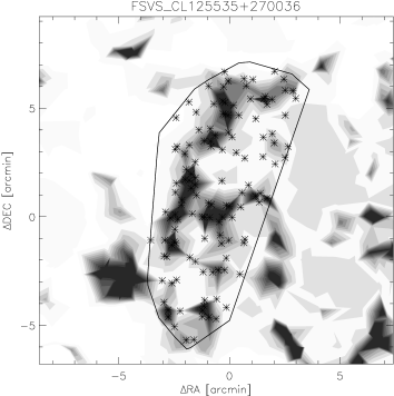
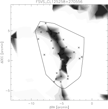
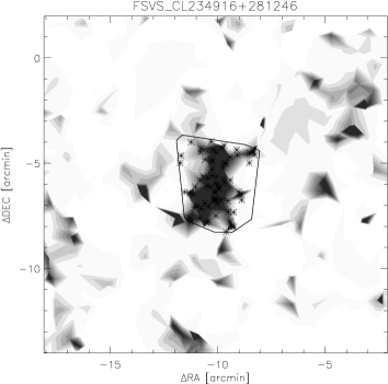
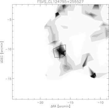
The FSVS cluster sample consists of 598 galaxy clusters and rich groups with $z<1$. The cluster detection method is morphologically unbiased, resulting in a sample of clusters with a wide range of spatial profiles. Figures 8 — 11 give some illustrative examples of the morphologies found in the sample — radially symmetric or elongated, compact or extended. The corresponding colour-magnitude diagrams serve to give an impression of the richness and brightness of these clusters.

Figure 8: FSVS$\_$CL125535$+$270036 — a highly elongated, rich (richness $=49$; see the text for definition) galaxy cluster at $z_{est}=0.279$, detected in Field 22. This cluster has very prominent substructure with galaxy groups tracing a filament-like structure. The cluster is $\sim$ $2.5h^{-1}$ Mpc by $1h^{-1}$ Mpc. Contours indicate the density of galaxies within the colour-magnitude filter of the cluster. The black polygon delineates the boundary of the cluster and asterisks denote its members. In the colour-magnitude diagram: asterisks denote galaxies that are identified as cluster members — they are within both the cluster boundary and the colour-magnitude filter (polygon); pluses denote galaxies within the cluster boundary but outside the colour-magnitude filter.

Figure 9: FSVS$\_$CL125258$+$270556 — a highly elongated, rich (richness $=37$) galaxy cluster at $z_{est}=0.470$, detected in Field 21. The cluster is $\sim$ $2.8h^{-1}$ Mpc by $1.5h^{-1}$ Mpc, but without the clumpiness of FSVS$\_$CL125535$+$270036. Although at higher redshift ($z_{est}=0.470$) its third brightest galaxy is only marginally fainter than in FSVS$\_$CL125535$+$270036, indicating higher intrinsic brightness. See the caption to Figure 8 for further details.

Figure 10: FSVS$\_$CL234916$+$281246 — an only marginally elongated, rich but compact cluster at $z_{est}=0.219$, detected in Field 79. Within the cluster boundary, multiple compact groups are still resolved indicating their relatively recent infall into the cluster. The cluster is $\sim$ $0.8h^{-1}$ Mpc in diameter. See the caption to Figure 8 for further details.

Figure 11: FSVS$\_$CL124755$+$255527 — a compact group at $z_{est}=0.067$ with a diameter of only $\sim$ $0.1h^{-1}$ Mpc, detected in Field 26. At such low redshifts ($z<0.1$), the FSVS cluster catalogue does not contain very rich and/or extended clusters owing to the relatively small size of the fields and the method not allowing detection of galaxy clusters larger than the window described by the data. However, considerable numbers of poor and compact groups have been detected. Like FSVS$\_$CL124755$+$255527, many of these groups trace a very narrow CRS in the colour-magnitude diagram, indicating that they contain only galaxies of similar age tracing the metallicity sequence. Such structures are very interesting subjects for studies of the chemical evolution because clusters are assembled from them. See the caption to Figure 8 for further details. Note, however, that in the colour-magnitude diagram there is an “anomalous” asterisk outside the colour-magnitude filter. We have added it because, exceptionally, the brightest galaxy of the group is brighter than the bright limit of the filter.

4.1 Richness distribution

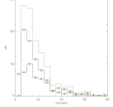
For our purposes, we define the richness of a galaxy cluster as the number of galaxies found within its spatial boundary and the colour-magnitude filter in the magnitude range $m_{3}<I<m_{3}+2$, where $m_{3}$ is the magnitude of the third brightest member galaxy. Although there are some similarities with the Abell richness definition, the above definition is unique for the FSVS clusters and cannot be directly translated into Abell richness. According to richness, a subsample of 395 poor ($<20$ members) clusters has been separated from the main sample. 117 of the poor clusters are at relatively high redshift ($z>0.4$) and due to cosmological dimming only the brighter part of the $m_{3}<I<m_{3}+2$ range is covered by our data. In such cases the richness is clearly underestimated.

The disadvantage of the calculation of richness from only a relatively small colour selection is a discrimination against clusters with a high fraction of blue galaxies that will not contribute to the galaxy count. This then leads to underestimation of the richness. However, inclusion of all galaxies within the cluster boundary would require a background substraction. The richness measure would then become prone to the usually large uncertainty in the estimate of the counts of background galaxies at the cluster position. A global background correction, used in the majority of richness estimates, is not appropriate owing to very strong local variations as found by Valotto, Moore & Lambas (2001) and readily visible in the colour-magnitude diagrams of the example FSVS clusters (Figures 8 and 9). In both examples the areas of the clusters are very similar, but, in the first example, the presence of multiple clusters at different redshifts produces a high local enhancement of the background galaxies. The richness measure adopted for the FSVS clusters can be considered as valid for the population of early-type galaxies in the clusters. Figure 12 illustrates the distribution of the richness of the FSVS clusters, divided into low and high redshift samples (where “low” signifies $z<0.4$).

Figure 12: The richness distribution of the FSVS cluster sample. For our purposes, we define the richness of a galaxy cluster as the number of galaxies found within its spatial boundary and the colour-magnitude filter in the magnitude range $m_{3}<I<m_{3}+2$, where $m_{3}$ is the magnitude of the third brightest member galaxy. The dotted histogram corresponds to all clusters, the solid line with squares to low redshift clusters ($z<0.4$), and the solid line with triangles to high redshift clusters ($z\geq 0.4$).

4.2 Redshift distribution

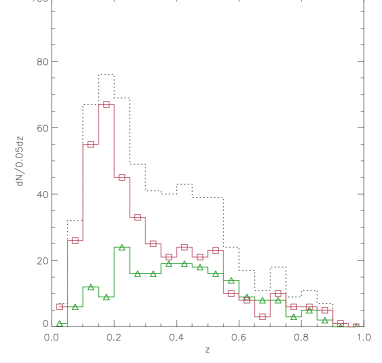
The 598 clusters detected in $21.75$ deg² of FSVS data correspond to a mean cluster density of $\sim 28$ deg^-2 and have a mean redshift of $\langle z\rangle=0.345$ (Figure 13). To compare our detection rate with, for example, those reported for SDSS data, which has a different depth, we need to consider the properties of the cluster luminosity function. The population of bright cluster galaxies (BCGs) is evident in the cluster luminosity function as a ”bump” at bright magnitudes that rises above the luminosity function of other cluster members (Lin & Mohr 2004; Hensen et al. 2005). As found by Hensen et al. (2005), the luminosity function of low- and intermediate-richness clusters cannot be well described by a Schechter function when BCGs are included; this function provides acceptable fits only for the richer systems where the fractional contribution of the central galaxies to the LF is small. The presence of the BCG population allows a high rate of cluster identification even in surveys detecting only a few (brightest) members. Consequently, up to a certain redshift, two surveys which are different in depth will still allow similar cluster detection rates.

We compared the cluster density in the FSVS Cluster Catalogue with the cluster sample derived from the SDSS data using the Cut-and-Enhance method (Goto et al. 2002). At $z<0.2$ the density in the FSVS sample is enhanced relative to that from the SDSS data, since FSVS includes poor groups, which have few bright galaxies excluding them from the shallower limits of the SDSS. However, in the restricted redshift range $0.2<z<0.3$, the cluster density of $6.3$ deg^-2 from FSVS is comparable to the $6.2$ deg^-2 found from SDSS data. In this transitional redshift range, the FSVS no longer allows the detection of poor groups but SDSS still has sufficient depth to see enough bright galaxies for positive cluster identification. At higher redshifts ($z>0.3$), the shallower SDSS begins to miss the galaxies in the bright tail of the luminosity function leading to a rapid decline in the cluster detection rate. Consequently, to carry out a comparison of both samples at $z>0.3$, the magnitude limit of the FSVS data would have to be restricted to match the SDSS. Instead, we deduce from the results at $z<0.3$ that both algorithms have similar detection efficiency.

Figure 13: The distribution of estimated redshifts in the FSVS cluster sample. The dotted line histogram corresponds to all clusters, the solid line with squares to poor clusters (richness $<20$), and the solid line with triangles to rich clusters (richness $\geq 20$).

The number of detected clusters $N_{cl}$ varies from field to field, ranging from 0 to 21. A small part of this variation is contributed by the difference in the limiting magnitudes arising from changes in observing conditions. However, the main contribution is due to the presence of voids and superclusters in the spatial distribution of galaxy clusters, also deduced from peaks in their redshift distribution if determined field by field. Figure 14 illustrates two examples of groupings of FSVS fields with prominent peaks in the redshift distribution of clusters, suggesting the presence of filament- or sheet-like structures.

Figure 14: The estimated redshift distribution of galaxy clusters in Fields 1–6 (top) and 8–12 (bottom).

4.3 Contamination by spurious clusters

Chance projections of galaxies similar in colour could cause some spurious detections in the cluster catalogue. A visual examination of the images cannot provide a reliable and repeatable check of the physical reality of the detected clusters. To avoid ambiguity, the reality of a cluster is judged by the presence of both a local overdensity and a well-defined linear CRS.

The partial maximised likelihood of a cluster with a positive contrast above background is

$$l(\mn@boldsymbol{x};{\mathcal{A}})>1.0$$ (9)

Adopting this value as a threshold to reject spurious clusters, we find a contamination level of $\sim 15\%$ distributed across the whole redshift range.

We then use a chi-square statistic as a measure of whether the linear fit to the colour-magnitude distribution of cluster members is acceptable — that is, whether we can consider the presence of a CRS to be believable.

We fit a linear relation to the putative CRS by minimising

$$\chi^{2}=\sum_{i=1}^{n}(y_{i}-(A+Bx_{i}))^{2}/\sigma_{i}^{2}$$ (10)

where $A$ and $B$ are the coefficients of the linear fit, $n$ is the number of cluster members and $\sigma_{i}$ is adopted as the photometric error of the galaxy colour. The values of A and B are extracted directly from the standard minimum squares fit without apriori restriction. We shall denote the minimised value of $\chi^{2}$ that results as $\chi^{2}_{CRS}$.

We then define a “CRS probability” as $P_{CRS}={\rm Pr}(\chi^{2}<\chi^{2}_{CRS})$ for a $\chi^{2}$ distribution with $n-3$ degrees of freedom.

We shall take values of this CRS probability above a specified threshold to indicate that the presence of a particular CRS is “believable.” The observed distribution of the values of the CRS probabilities is shown in Figure 15. There is a minimum in the distribution at $P_{CRS}\sim 0.4$, which, unlike the local minimum at $P_{CRS}\sim 0.2$, appears to genuinely mark a transition from generally decreasing to generally increasing. We cautiously but plausibly interpret the transition as being from predominantly spurious clusters ($P_{CRS}<0.4$) to predominantly real clusters ($P_{CRS}\geq 0.4$). We have therefore adopted the value of $P_{CRS}=0.4$ as the threshold.

Clearly, this $\chi^{2}$ procedure is not statistically rigorous because the threshold of $P_{CRS}=0.4$ is set by judgement and also because of bias to the $\chi^{2}$-minimisation and calculation of $P_{CRS}$ that results from the imposition of the colour-magnitude filter. Nevertheless, the procedure provides a clearly-defined criterion for assessing whether a CRS is believable. We might find in future that the chosen threshold of $0.4$ will need some revision.

Figure 15: Distribution of the “CRS probability,” $P_{CRS}={\rm Pr}(\chi^{2}<\chi^{2}_{CRS})$ for a $\chi^{2}$ distribution with $n-3$ degrees of freedom. The value $P_{CRS}\sim 0.4$ at which a miminum is seen is adopted as the threshold for a believable CRS.

Considering the lack of a reliable CRS to be an indication that a cluster is spurious, the contamination of the sample has been estimated to be $\sim 31\%$. Nevertheless, the level of contamination varies strongly with redshift. Figure 16 shows that very few of the higher redshift ($z>0.4$) clusters are suspected of being spurious. Furthermore, many of the rejected clusters have a very high spatial likelihood (very high values of $l(\mn@boldsymbol{x};{\mathcal{A}})$) suggesting that our test of the presence of a linear CRS is biased against rich, low-redshift clusters. The $\chi^{2}_{CRS}$ of these clusters is inflated by a large population of faint member galaxies occupying much broader colour-space. To overcome this limitation, only clusters with an “unbelievable” CRS combined with likelihood $l(\mn@boldsymbol{x};{\mathcal{A}})$ below the median are rejected. This parameter combination (CRS probability $<0.4$ and $l(\mn@boldsymbol{x};{\mathcal{A}})<3.28$) rejects $12.8\%$ of clusters as spurious.

Figure 16: Plot of cluster spatial likelihood $l(\mn@boldsymbol{x};{\mathcal{A}})$ versus redshift. Diamonds indicate clusters with an “unbelievable” CRS (CRS probability $P_{CRS}<0.4$); crosses mark the remaining cluster population. The horizontal solid line indicates the median likelihood.

Figure 17 illustrates the overall rejection region that is defined by the restrictions on spatial likelihood and CRS probability ($P_{CRS}<0.4$ and $l(\mn@boldsymbol{x};{\mathcal{A}})<3.28$, or $l(\mn@boldsymbol{x};{\mathcal{A}})<1.0$). The overall contamination by spurious clusters is then estimated to be below $24\%$.

Figure 17: Plot of cluster spatial likelihood $l(\mn@boldsymbol{x};{\mathcal{A}})$ versus CRS probability. All clusters below the solid line are rejected as spurious.

The FSVS cluster catalogue is dominated by poor clusters and groups that may lack central bright galaxies and that show small diversity in magnitude. Consequently, many of the clusters found to lack a strong CRS may still be real and the estimated contamination has to be considered to be an upper limit.

5 The Catalogue

A wide range of parameters has been derived for every detected cluster. The catalogue given here, Table 4, contains only the most basic information such as ID, position and estimated redshift.

Table 4: The basic FSVS cluster catalogue. The columns are: (1) identification of the cluster; (2) and (3) RA, Dec (J2000) of the cluster centre, defined as the mean position of its members; (4) estimated redshift, $z_{est}$.

ID	RA(J2000)	Dec(J2000)	$z_{est}$	ID	RA(J2000)	Dec(J2000)	$z_{est}$
FSVS$\_$CL234208$+$265328	23:42:08	26:53:28	0.13	FSVS$\_$CL234251$+$270509	23:42:51	27:05:09	0.15
FSVS$\_$CL234146$+$265554	23:41:46	26:55:54	0.21	FSVS$\_$CL234208$+$270501	23:42:08	27:05:01	0.22
FSVS$\_$CL234201$+$271109	23:42:01	27:11:09	0.39	FSVS$\_$CL234057$+$270648	23:40:57	27:06:48	0.53
FSVS$\_$CL234208$+$270739	23:42:08	27:07:39	0.66	FSVS$\_$CL234150$+$265516	23:41:50	26:55:16	0.94
FSVS$\_$CL234326$+$270343	23:43:26	27:03:43	0.11	FSVS$\_$CL234404$+$270134	23:44:04	27:01:34	0.11
FSVS$\_$CL234439$+$270201	23:44:39	27:02:01	0.21	FSVS$\_$CL234410$+$270022	23:44:10	27:00:22	0.26
FSVS$\_$CL234505$+$265235	23:45:05	26:52:35	0.21	FSVS$\_$CL234441$+$270217	23:44:41	27:02:17	0.37
FSVS$\_$CL234448$+$270754	23:44:48	27:07:54	0.45	FSVS$\_$CL234500$+$265648	23:45:00	26:56:48	0.52
FSVS$\_$CL234455$+$265542	23:44:55	26:55:42	0.58	FSVS$\_$CL234449$+$270551	23:44:49	27:05:51	0.52
FSVS$\_$CL234439$+$270420	23:44:39	27:04:20	0.79	FSVS$\_$CL234624$+$265637	23:46:24	26:56:37	0.08
FSVS$\_$CL234610$+$270123	23:46:10	27:01:23	0.15	FSVS$\_$CL234621$+$265307	23:46:21	26:53:07	0.07
FSVS$\_$CL234600$+$271757	23:46:00	27:17:57	0.16	FSVS$\_$CL234646$+$270852	23:46:46	27:08:52	0.14
FSVS$\_$CL234614$+$265034	23:46:14	26:50:34	0.19	FSVS$\_$CL234540$+$265115	23:45:40	26:51:15	0.27
FSVS$\_$CL234607$+$265222	23:46:07	26:52:22	0.19	FSVS$\_$CL234658$+$270857	23:46:58	27:08:57	0.22
FSVS$\_$CL234607$+$265323	23:46:07	26:53:23	0.51	FSVS$\_$CL234621$+$270202	23:46:21	27:02:02	0.33
FSVS$\_$CL234613$+$265333	23:46:13	26:53:33	0.35	FSVS$\_$CL234631$+$265834	23:46:31	26:58:34	0.38
FSVS$\_$CL234445$+$270756	23:44:45	27:07:56	0.40	FSVS$\_$CL234545$+$270456	23:45:45	27:04:56	0.54
FSVS$\_$CL234537$+$270728	23:45:37	27:07:28	0.70	FSVS$\_$CL234648$+$273728	23:46:48	27:37:28	0.24
FSVS$\_$CL234610$+$272345	23:46:10	27:23:45	0.29	FSVS$\_$CL234635$+$275013	23:46:35	27:50:13	0.33
FSVS$\_$CL234641$+$273702	23:46:41	27:37:02	0.33	FSVS$\_$CL234607$+$272123	23:46:07	27:21:23	0.49
FSVS$\_$CL234604$+$272231	23:46:04	27:22:31	0.55	FSVS$\_$CL234559$+$273049	23:45:59	27:30:49	0.62
FSVS$\_$CL234557$+$272616	23:45:57	27:26:16	0.84	FSVS$\_$CL234639$+$275029	23:46:39	27:50:29	0.80
FSVS$\_$CL234430$+$274709	23:44:30	27:47:09	0.14	FSVS$\_$CL234417$+$272714	23:44:17	27:27:14	0.14
FSVS$\_$CL234456$+$272255	23:44:56	27:22:55	0.17	FSVS$\_$CL234437$+$274550	23:44:37	27:45:50	0.19
FSVS$\_$CL234337$+$273622	23:43:37	27:36:22	0.40	FSVS$\_$CL234453$+$272254	23:44:53	27:22:54	0.43
FSVS$\_$CL234312$+$272327	23:43:12	27:23:27	0.51	FSVS$\_$CL234351$+$272825	23:43:51	27:28:25	0.79
FSVS$\_$CL234138$+$273954	23:41:38	27:39:54	0.08	FSVS$\_$CL234055$+$273202	23:40:55	27:32:02	0.10
FSVS$\_$CL234100$+$272828	23:41:00	27:28:28	0.22	FSVS$\_$CL234134$+$271950	23:41:34	27:19:50	0.17
FSVS$\_$CL234247$+$272400	23:42:47	27:24:00	0.46	FSVS$\_$CL234144$+$273214	23:41:44	27:32:14	0.49
FSVS$\_$CL234141$+$273135	23:41:41	27:31:35	0.53	FSVS$\_$CL234137$+$273143	23:41:37	27:31:43	0.79
FSVS$\_$CL022856$+$144800	02:28:56	14:48:00	0.20	FSVS$\_$CL022956$+$145701	02:29:56	14:57:01	0.27
FSVS$\_$CL022931$+$143738	02:29:31	14:37:38	0.27	FSVS$\_$CL022925$+$144632	02:29:25	14:46:32	0.27
FSVS$\_$CL022855$+$144801	02:28:55	14:48:01	0.42	FSVS$\_$CL022813$+$144547	02:28:13	14:45:47	0.57
FSVS$\_$CL022844$+$144712	02:28:44	14:47:12	0.56	FSVS$\_$CL022947$+$143524	02:29:47	14:35:24	0.72
FSVS$\_$CL023117$+$150515	02:31:17	15:05:15	0.18	FSVS$\_$CL023101$+$144945	02:31:01	14:49:45	0.19
FSVS$\_$CL023057$+$144500	02:30:57	14:45:00	0.38	FSVS$\_$CL023001$+$145656	02:30:01	14:56:56	0.41
FSVS$\_$CL022957$+$145747	02:29:57	14:57:47	0.48	FSVS$\_$CL023509$+$150306	02:35:09	15:03:06	0.07
FSVS$\_$CL023420$+$151633	02:34:20	15:16:33	0.16	FSVS$\_$CL023412$+$150004	02:34:12	15:00:04	0.18
FSVS$\_$CL023341$+$151137	02:33:41	15:11:37	0.39	FSVS$\_$CL023332$+$145904	02:33:32	14:59:04	0.47
FSVS$\_$CL023432$+$151326	02:34:32	15:13:26	0.72	FSVS$\_$CL023647$+$152254	02:36:47	15:22:54	0.18
FSVS$\_$CL023643$+$152354	02:36:43	15:23:54	0.26	FSVS$\_$CL023621$+$151025	02:36:21	15:10:25	0.44
FSVS$\_$CL023635$+$151533	02:36:35	15:15:33	0.69	FSVS$\_$CL023845$+$153632	02:38:45	15:36:32	0.19
FSVS$\_$CL023832$+$153907	02:38:32	15:39:07	0.21	FSVS$\_$CL023816$+$152247	02:38:16	15:22:47	0.22
FSVS$\_$CL074721$+$205219	07:47:21	20:52:19	0.14	FSVS$\_$CL074808$+$210159	07:48:08	21:01:59	0.14
FSVS$\_$CL074813$+$205529	07:48:13	20:55:29	0.18	FSVS$\_$CL074807$+$210550	07:48:07	21:05:50	0.27
FSVS$\_$CL074725$+$204939	07:47:25	20:49:39	0.28	FSVS$\_$CL075014$+$205839	07:50:14	20:58:39	0.08
FSVS$\_$CL074922$+$204039	07:49:22	20:40:39	0.16	FSVS$\_$CL075053$+$205247	07:50:53	20:52:47	0.16
FSVS$\_$CL075100$+$204842	07:51:00	20:48:42	0.19	FSVS$\_$CL075034$+$205510	07:50:34	20:55:10	0.24
FSVS$\_$CL075032$+$205545	07:50:32	20:55:45	0.36	FSVS$\_$CL075055$+$210542	07:50:55	21:05:42	0.36
FSVS$\_$CL075053$+$205221	07:50:53	20:52:21	0.51	FSVS$\_$CL075155$+$203343	07:51:55	20:33:43	0.08
FSVS$\_$CL075148$+$204634	07:51:48	20:46:34	0.09	FSVS$\_$CL075307$+$204636	07:53:07	20:46:36	0.18
FSVS$\_$CL075220$+$204328	07:52:20	20:43:28	0.14	FSVS$\_$CL075254$+$203123	07:52:54	20:31:23	0.27
FSVS$\_$CL075314$+$203637	07:53:14	20:36:37	0.31	FSVS$\_$CL075202$+$204352	07:52:02	20:43:52	0.44
FSVS$\_$CL075455$+$203646	07:54:55	20:36:46	0.09	FSVS$\_$CL075348$+$204158	07:53:48	20:41:58	0.15
FSVS$\_$CL075406$+$203207	07:54:06	20:32:07	0.18	FSVS$\_$CL075415$+$203426	07:54:15	20:34:26	0.20
FSVS$\_$CL075529$+$204532	07:55:29	20:45:32	0.29	FSVS$\_$CL075504$+$204520	07:55:04	20:45:20	0.44
FSVS$\_$CL075430$+$202712	07:54:30	20:27:12	0.57	FSVS$\_$CL075712$+$202015	07:57:12	20:20:15	0.19

Table 4: Continued.

ID	RA(J2000)	Dec(J2000)	$z_{est}$	ID	RA(J2000)	Dec(J2000)	$z_{est}$
FSVS$\_$CL075656$+$203049	07:56:56	20:30:49	0.41	FSVS$\_$CL075702$+$203421	07:57:02	20:34:21	0.86
FSVS$\_$CL075908$+$205955	07:59:08	20:59:55	0.07	FSVS$\_$CL075842$+$210256	07:58:42	21:02:56	0.14
FSVS$\_$CL075853$+$211245	07:58:53	21:12:45	0.20	FSVS$\_$CL075846$+$205104	07:58:46	20:51:04	0.22
FSVS$\_$CL075801$+$205055	07:58:01	20:50:55	0.25	FSVS$\_$CL075858$+$210527	07:58:58	21:05:27	0.22
FSVS$\_$CL075828$+$210023	07:58:28	21:00:23	0.31	FSVS$\_$CL075807$+$205146	07:58:07	20:51:46	0.43
FSVS$\_$CL075808$+$211321	07:58:08	21:13:21	0.52	FSVS$\_$CL125049$+$264834	12:50:49	26:48:34	0.41
FSVS$\_$CL125006$+$270117	12:50:06	27:01:17	0.12	FSVS$\_$CL124938$+$265301	12:49:38	26:53:01	0.14
FSVS$\_$CL124915$+$264620	12:49:15	26:46:20	0.30	FSVS$\_$CL124917$+$271153	12:49:17	27:11:53	0.28
FSVS$\_$CL124955$+$264645	12:49:55	26:46:45	0.37	FSVS$\_$CL124842$+$270735	12:48:42	27:07:35	0.44
FSVS$\_$CL124845$+$265335	12:48:45	26:53:35	0.52	FSVS$\_$CL124854$+$271449	12:48:54	27:14:49	0.52
FSVS$\_$CL124903$+$271259	12:49:03	27:12:59	0.57	FSVS$\_$CL124918$+$271135	12:49:18	27:11:35	0.71
FSVS$\_$CL125315$+$271527	12:53:15	27:15:27	0.25	FSVS$\_$CL125357$+$265044	12:53:57	26:50:44	0.31
FSVS$\_$CL125258$+$270556	12:52:58	27:05:56	0.45	FSVS$\_$CL125332$+$271332	12:53:32	27:13:32	0.42
FSVS$\_$CL125312$+$265349	12:53:12	26:53:49	0.45	FSVS$\_$CL125300$+$272116	12:53:00	27:21:16	0.45
FSVS$\_$CL125539$+$265122	12:55:39	26:51:22	0.12	FSVS$\_$CL125511$+$265510	12:55:11	26:55:10	0.10
FSVS$\_$CL125627$+$264800	12:56:27	26:48:00	0.09	FSVS$\_$CL125524$+$265800	12:55:24	26:58:00	0.41
FSVS$\_$CL125535$+$264549	12:55:35	26:45:49	0.17	FSVS$\_$CL125602$+$265121	12:56:02	26:51:21	0.12
FSVS$\_$CL125540$+$264517	12:55:40	26:45:17	0.16	FSVS$\_$CL125535$+$270036	12:55:35	27:00:36	0.27
FSVS$\_$CL125423$+$265107	12:54:23	26:51:07	0.24	FSVS$\_$CL125636$+$270837	12:56:36	27:08:37	0.25
FSVS$\_$CL125611$+$265756	12:56:11	26:57:56	0.27	FSVS$\_$CL125550$+$270450	12:55:50	27:04:50	0.36
FSVS$\_$CL125555$+$271626	12:55:55	27:16:26	0.41	FSVS$\_$CL125531$+$265746	12:55:31	26:57:46	0.59
FSVS$\_$CL125628$+$265333	12:56:28	26:53:33	0.86	FSVS$\_$CL125428$+$261050	12:54:28	26:10:50	0.15
FSVS$\_$CL125520$+$261912	12:55:20	26:19:12	0.15	FSVS$\_$CL125515$+$261842	12:55:15	26:18:42	0.22
FSVS$\_$CL125559$+$260443	12:55:59	26:04:43	0.18	FSVS$\_$CL125544$+$262518	12:55:44	26:25:18	0.15
FSVS$\_$CL125632$+$262418	12:56:32	26:24:18	0.19	FSVS$\_$CL125634$+$260833	12:56:34	26:08:33	0.17
FSVS$\_$CL125438$+$261716	12:54:38	26:17:16	0.16	FSVS$\_$CL125513$+$262023	12:55:13	26:20:23	0.31
FSVS$\_$CL125537$+$262409	12:55:37	26:24:09	0.29	FSVS$\_$CL125539$+$262545	12:55:39	26:25:45	0.39
FSVS$\_$CL125442$+$262109	12:54:42	26:21:09	0.46	FSVS$\_$CL125556$+$260810	12:55:56	26:08:10	0.60
FSVS$\_$CL125617$+$262337	12:56:17	26:23:37	0.53	FSVS$\_$CL125335$+$261534	12:53:35	26:15:34	0.07
FSVS$\_$CL125332$+$261305	12:53:32	26:13:05	0.09	FSVS$\_$CL125418$+$260931	12:54:18	26:09:31	0.06
FSVS$\_$CL125322$+$262508	12:53:22	26:25:08	0.13	FSVS$\_$CL125358$+$261956	12:53:58	26:19:56	0.12
FSVS$\_$CL125327$+$263249	12:53:27	26:32:49	0.12	FSVS$\_$CL125317$+$263249	12:53:17	26:32:49	0.15
FSVS$\_$CL125411$+$261259	12:54:11	26:12:59	0.18	FSVS$\_$CL125222$+$261612	12:52:22	26:16:12	0.26
FSVS$\_$CL125316$+$260912	12:53:16	26:09:12	0.24	FSVS$\_$CL125255$+$261808	12:52:55	26:18:08	0.36
FSVS$\_$CL125353$+$261739	12:53:53	26:17:39	0.30	FSVS$\_$CL125312$+$261217	12:53:12	26:12:17	0.52
FSVS$\_$CL125318$+$260652	12:53:18	26:06:52	0.52	FSVS$\_$CL125326$+$262052	12:53:26	26:20:52	0.51
FSVS$\_$CL125307$+$261714	12:53:07	26:17:14	0.67	FSVS$\_$CL125039$+$261548	12:50:39	26:15:48	0.18
FSVS$\_$CL125143$+$263329	12:51:43	26:33:29	0.12	FSVS$\_$CL125150$+$263419	12:51:50	26:34:19	0.11
FSVS$\_$CL124958$+$262347	12:49:58	26:23:47	0.14	FSVS$\_$CL125028$+$261838	12:50:28	26:18:38	0.21
FSVS$\_$CL125017$+$262617	12:50:17	26:26:17	0.12	FSVS$\_$CL125050$+$262435	12:50:50	26:24:35	0.20
FSVS$\_$CL124955$+$261746	12:49:55	26:17:46	0.20	FSVS$\_$CL125012$+$261104	12:50:12	26:11:04	0.25
FSVS$\_$CL125109$+$261151	12:51:09	26:11:51	0.27	FSVS$\_$CL125048$+$263418	12:50:48	26:34:18	0.30
FSVS$\_$CL125035$+$261332	12:50:35	26:13:32	0.38	FSVS$\_$CL125006$+$260853	12:50:06	26:08:53	0.37
FSVS$\_$CL125030$+$262743	12:50:30	26:27:43	0.33	FSVS$\_$CL125009$+$260931	12:50:09	26:09:31	0.41
FSVS$\_$CL125145$+$263824	12:51:45	26:38:24	0.37	FSVS$\_$CL125030$+$262535	12:50:30	26:25:35	0.46
FSVS$\_$CL125007$+$261031	12:50:07	26:10:31	0.45	FSVS$\_$CL125140$+$262640	12:51:40	26:26:40	0.62
FSVS$\_$CL125028$+$262052	12:50:28	26:20:52	0.73	FSVS$\_$CL124929$+$255843	12:49:29	25:58:43	0.16
FSVS$\_$CL124755$+$255527	12:47:55	25:55:27	0.08	FSVS$\_$CL124925$+$260755	12:49:25	26:07:55	0.14
FSVS$\_$CL124904$+$255734	12:49:04	25:57:34	0.28	FSVS$\_$CL124943$+$261754	12:49:43	26:17:54	0.53
FSVS$\_$CL162235$+$263052	16:22:35	26:30:52	0.17	FSVS$\_$CL162421$+$264423	16:24:21	26:44:23	0.12
FSVS$\_$CL162424$+$262315	16:24:24	26:23:15	0.14	FSVS$\_$CL162339$+$263433	16:23:39	26:34:33	0.39
FSVS$\_$CL162415$+$263854	16:24:15	26:38:54	0.15	FSVS$\_$CL162412$+$263008	16:24:12	26:30:08	0.37
FSVS$\_$CL162358$+$264914	16:23:58	26:49:14	0.71	FSVS$\_$CL162420$+$263719	16:24:20	26:37:19	0.63
FSVS$\_$CL162434$+$263800	16:24:34	26:38:00	0.80	FSVS$\_$CL162154$+$262742	16:21:54	26:27:42	0.10
FSVS$\_$CL162229$+$264730	16:22:29	26:47:30	0.16	FSVS$\_$CL162131$+$262758	16:21:31	26:27:58	0.13
FSVS$\_$CL162231$+$262657	16:22:31	26:26:57	0.18	FSVS$\_$CL162045$+$262549	16:20:45	26:25:49	0.12
FSVS$\_$CL162200$+$262722	16:22:00	26:27:22	0.25	FSVS$\_$CL162108$+$262732	16:21:08	26:27:32	0.28
FSVS$\_$CL162119$+$264758	16:21:19	26:47:58	0.68	FSVS$\_$CL162508$+$263444	16:25:08	26:34:44	0.06
FSVS$\_$CL162518$+$262857	16:25:18	26:28:57	0.11	FSVS$\_$CL162510$+$262634	16:25:10	26:26:34	0.24
FSVS$\_$CL162515$+$262418	16:25:15	26:24:18	0.37	FSVS$\_$CL162520$+$262409	16:25:20	26:24:09	0.40

Table 4: Continued.

ID	RA(J2000)	Dec(J2000)	$z_{est}$	ID	RA(J2000)	Dec(J2000)	$z_{est}$
FSVS$\_$CL162855$+$263430	16:28:55	26:34:30	0.13	FSVS$\_$CL162832$+$263640	16:28:32	26:36:40	0.28
FSVS$\_$CL162849$+$263741	16:28:49	26:37:41	0.31	FSVS$\_$CL162810$+$263537	16:28:10	26:35:37	0.35
FSVS$\_$CL162706$+$263339	16:27:06	26:33:39	0.36	FSVS$\_$CL172015$+$263858	17:20:15	26:38:58	0.10
FSVS$\_$CL172110$+$262919	17:21:10	26:29:19	0.17	FSVS$\_$CL172059$+$265741	17:20:59	26:57:41	0.13
FSVS$\_$CL171930$+$263253	17:19:30	26:32:53	0.22	FSVS$\_$CL172107$+$265336	17:21:07	26:53:36	0.27
FSVS$\_$CL172008$+$264112	17:20:08	26:41:12	0.35	FSVS$\_$CL171930$+$263812	17:19:30	26:38:12	0.39
FSVS$\_$CL171914$+$264335	17:19:14	26:43:35	0.49	FSVS$\_$CL171932$+$262948	17:19:32	26:29:48	0.50
FSVS$\_$CL172030$+$261200	17:20:30	26:12:00	0.09	FSVS$\_$CL172004$+$261810	17:20:04	26:18:10	0.03
FSVS$\_$CL171901$+$260202	17:19:01	26:02:02	0.11	FSVS$\_$CL172017$+$255048	17:20:17	25:50:48	0.20
FSVS$\_$CL172027$+$261323	17:20:27	26:13:23	0.13	FSVS$\_$CL171852$+$255236	17:18:52	25:52:36	0.18
FSVS$\_$CL172020$+$260951	17:20:20	26:09:51	0.17	FSVS$\_$CL171853$+$255038	17:18:53	25:50:38	0.30
FSVS$\_$CL172046$+$261308	17:20:46	26:13:08	0.22	FSVS$\_$CL171930$+$260325	17:19:30	26:03:25	0.28
FSVS$\_$CL172042$+$260436	17:20:42	26:04:36	0.32	FSVS$\_$CL171931$+$261901	17:19:31	26:19:01	0.36
FSVS$\_$CL171849$+$255300	17:18:49	25:53:00	0.48	FSVS$\_$CL172048$+$254819	17:20:48	25:48:19	0.55
FSVS$\_$CL171857$+$255213	17:18:57	25:52:13	0.84	FSVS$\_$CL172053$+$272314	17:20:53	27:23:14	0.06
FSVS$\_$CL172037$+$271636	17:20:37	27:16:36	0.09	FSVS$\_$CL172032$+$271607	17:20:32	27:16:07	0.20
FSVS$\_$CL172109$+$265947	17:21:09	26:59:47	0.18	FSVS$\_$CL172105$+$271911	17:21:05	27:19:11	0.15
FSVS$\_$CL171934$+$271032	17:19:34	27:10:32	0.22	FSVS$\_$CL171944$+$271429	17:19:44	27:14:29	0.20
FSVS$\_$CL171945$+$271051	17:19:45	27:10:51	0.39	FSVS$\_$CL171942$+$270906	17:19:42	27:09:06	0.62
FSVS$\_$CL172010$+$271202	17:20:10	27:12:02	0.78	FSVS$\_$CL171937$+$270740	17:19:37	27:07:40	0.69
FSVS$\_$CL171944$+$265634	17:19:44	26:56:34	0.87	FSVS$\_$CL172030$+$274013	17:20:30	27:40:13	0.18
FSVS$\_$CL172100$+$273642	17:21:00	27:36:42	0.12	FSVS$\_$CL172109$+$274329	17:21:09	27:43:29	0.19
FSVS$\_$CL172123$+$274750	17:21:23	27:47:50	0.21	FSVS$\_$CL172125$+$274456	17:21:25	27:44:56	0.27
FSVS$\_$CL172124$+$274457	17:21:24	27:44:57	0.33	FSVS$\_$CL172015$+$273823	17:20:15	27:38:23	0.37
FSVS$\_$CL171936$+$273208	17:19:36	27:32:08	0.52	FSVS$\_$CL172004$+$273733	17:20:04	27:37:33	0.62
FSVS$\_$CL172003$+$273338	17:20:03	27:33:38	0.85	FSVS$\_$CL172026$+$274516	17:20:26	27:45:16	0.87
FSVS$\_$CL025812$+$192245	02:58:12	19:22:45	0.39	FSVS$\_$CL025820$+$193519	02:58:20	19:35:19	0.46
FSVS$\_$CL025730$+$193637	02:57:30	19:36:37	0.47	FSVS$\_$CL025812$+$193852	02:58:12	19:38:52	0.66
FSVS$\_$CL025817$+$193356	02:58:17	19:33:56	0.68	FSVS$\_$CL030348$+$193451	03:03:48	19:34:51	0.04
FSVS$\_$CL030327$+$194215	03:03:27	19:42:15	0.09	FSVS$\_$CL030304$+$193601	03:03:04	19:36:01	0.19
FSVS$\_$CL030327$+$194214	03:03:27	19:42:14	0.22	FSVS$\_$CL030233$+$193522	03:02:33	19:35:22	0.29
FSVS$\_$CL030258$+$195007	03:02:58	19:50:07	0.47	FSVS$\_$CL030239$+$192933	03:02:39	19:29:33	0.46
FSVS$\_$CL030345$+$193647	03:03:45	19:36:47	0.44	FSVS$\_$CL030251$+$192415	03:02:51	19:24:15	0.53
FSVS$\_$CL030244$+$194036	03:02:44	19:40:36	0.46	FSVS$\_$CL030257$+$192619	03:02:57	19:26:19	0.54
FSVS$\_$CL030537$+$195347	03:05:37	19:53:47	0.11	FSVS$\_$CL030449$+$193756	03:04:49	19:37:56	0.33
FSVS$\_$CL030508$+$193023	03:05:08	19:30:23	0.41	FSVS$\_$CL030855$+$194515	03:08:55	19:45:15	0.17
FSVS$\_$CL031105$+$193428	03:11:05	19:34:28	0.12	FSVS$\_$CL031103$+$194936	03:11:03	19:49:36	0.41
FSVS$\_$CL071453$+$200648	07:14:53	20:06:48	0.07	FSVS$\_$CL071449$+$200245	07:14:49	20:02:45	0.16
FSVS$\_$CL071503$+$204801	07:15:03	20:48:01	0.53	FSVS$\_$CL071443$+$210911	07:14:43	21:09:11	0.15
FSVS$\_$CL071458$+$211228	07:14:58	21:12:28	0.15	FSVS$\_$CL071520$+$211013	07:15:20	21:10:13	0.19
FSVS$\_$CL071402$+$210027	07:14:02	21:00:27	0.47	FSVS$\_$CL071405$+$205947	07:14:05	20:59:47	0.57
FSVS$\_$CL071519$+$211256	07:15:19	21:12:56	0.59	FSVS$\_$CL071535$+$212351	07:15:35	21:23:51	0.78
FSVS$\_$CL071444$+$214622	07:14:44	21:46:22	0.12	FSVS$\_$CL071558$+$214733	07:15:58	21:47:33	0.13
FSVS$\_$CL071550$+$214842	07:15:50	21:48:42	0.16	FSVS$\_$CL071535$+$214256	07:15:35	21:42:56	0.21
FSVS$\_$CL071520$+$220013	07:15:20	22:00:13	0.28	FSVS$\_$CL071530$+$214206	07:15:30	21:42:06	0.32
FSVS$\_$CL071436$+$214204	07:14:36	21:42:04	0.29	FSVS$\_$CL071521$+$214116	07:15:21	21:41:16	0.66
FSVS$\_$CL071405$+$221159	07:14:05	22:11:59	0.20	FSVS$\_$CL071508$+$223233	07:15:08	22:32:33	0.22
FSVS$\_$CL071402$+$221709	07:14:02	22:17:09	0.19	FSVS$\_$CL071502$+$223716	07:15:02	22:37:16	0.40
FSVS$\_$CL071431$+$221018	07:14:31	22:10:18	0.48	FSVS$\_$CL071550$+$223003	07:15:50	22:30:03	0.70
FSVS$\_$CL071516$+$234824	07:15:16	23:48:24	0.12	FSVS$\_$CL071523$+$234841	07:15:23	23:48:41	0.20
FSVS$\_$CL071422$+$233547	07:14:22	23:35:47	0.28	FSVS$\_$CL071455$+$232606	07:14:55	23:26:06	0.38
FSVS$\_$CL071357$+$233017	07:13:57	23:30:17	0.66	FSVS$\_$CL071536$+$232254	07:15:36	23:22:54	0.57
FSVS$\_$CL100031$+$200527	10:00:31	20:05:27	0.13	FSVS$\_$CL095926$+$205923	09:59:26	20:59:23	0.16
FSVS$\_$CL100005$+$211017	10:00:05	21:10:17	0.21	FSVS$\_$CL100034$+$212432	10:00:34	21:24:32	0.24
FSVS$\_$CL100007$+$211843	10:00:07	21:18:43	0.21	FSVS$\_$CL095943$+$210107	09:59:43	21:01:07	0.36
FSVS$\_$CL095906$+$210815	09:59:06	21:08:15	0.38	FSVS$\_$CL100019$+$210127	10:00:19	21:01:27	0.52
FSVS$\_$CL095857$+$211050	09:58:57	21:10:50	0.54	FSVS$\_$CL100036$+$215229	10:00:36	21:52:29	0.13

Table 4: Continued.

ID	RA(J2000)	Dec(J2000)	$z_{est}$	ID	RA(J2000)	Dec(J2000)	$z_{est}$
FSVS$\_$CL100002$+$214502	10:00:02	21:45:02	0.16	FSVS$\_$CL100042$+$215711	10:00:42	21:57:11	0.16
FSVS$\_$CL100007$+$215028	10:00:07	21:50:28	0.18	FSVS$\_$CL095853$+$213303	09:58:53	21:33:03	0.36
FSVS$\_$CL095947$+$214953	09:59:47	21:49:53	0.24	FSVS$\_$CL100045$+$215145	10:00:45	21:51:45	0.27
FSVS$\_$CL100026$+$215049	10:00:26	21:50:49	0.24	FSVS$\_$CL100039$+$220259	10:00:39	22:02:59	0.32
FSVS$\_$CL100036$+$215038	10:00:36	21:50:38	0.41	FSVS$\_$CL100041$+$215653	10:00:41	21:56:53	0.32
FSVS$\_$CL100050$+$224858	10:00:50	22:48:58	0.06	FSVS$\_$CL095852$+$230036	09:58:52	23:00:36	0.19
FSVS$\_$CL095941$+$224640	09:59:41	22:46:40	0.17	FSVS$\_$CL095922$+$225704	09:59:22	22:57:04	0.16
FSVS$\_$CL100038$+$224949	10:00:38	22:49:49	0.23	FSVS$\_$CL100007$+$230328	10:00:07	23:03:28	0.31
FSVS$\_$CL095902$+$225638	09:59:02	22:56:38	0.39	FSVS$\_$CL095943$+$231315	09:59:43	23:13:15	0.37
FSVS$\_$CL100046$+$225357	10:00:46	22:53:57	0.45	FSVS$\_$CL100103$+$224457	10:01:03	22:44:57	0.46
FSVS$\_$CL100041$+$224931	10:00:41	22:49:31	0.48	FSVS$\_$CL100015$+$230224	10:00:15	23:02:24	0.48
FSVS$\_$CL100024$+$230153	10:00:24	23:01:53	0.52	FSVS$\_$CL162423$+$265838	16:24:23	26:58:38	0.12
FSVS$\_$CL162328$+$272231	16:23:28	27:22:31	0.28	FSVS$\_$CL162423$+$271140	16:24:23	27:11:40	0.34
FSVS$\_$CL162241$+$265902	16:22:41	26:59:02	0.36	FSVS$\_$CL162417$+$271119	16:24:17	27:11:19	0.37
FSVS$\_$CL162334$+$265947	16:23:34	26:59:47	0.43	FSVS$\_$CL162430$+$265610	16:24:30	26:56:10	0.57
FSVS$\_$CL162430$+$270645	16:24:30	27:06:45	0.60	FSVS$\_$CL162308$+$265847	16:23:08	26:58:47	0.79
FSVS$\_$CL162016$+$270018	16:20:16	27:00:18	0.12	FSVS$\_$CL162115$+$265745	16:21:15	26:57:45	0.18
FSVS$\_$CL162138$+$270643	16:21:38	27:06:43	0.16	FSVS$\_$CL162020$+$265835	16:20:20	26:58:35	0.20
FSVS$\_$CL162044$+$270340	16:20:44	27:03:40	0.22	FSVS$\_$CL162030$+$265459	16:20:30	26:54:59	0.25
FSVS$\_$CL162045$+$270739	16:20:45	27:07:39	0.15	FSVS$\_$CL162031$+$270019	16:20:31	27:00:19	0.26
FSVS$\_$CL162144$+$270952	16:21:44	27:09:52	0.40	FSVS$\_$CL162012$+$265452	16:20:12	26:54:52	0.34
FSVS$\_$CL162104$+$265842	16:21:04	26:58:42	0.32	FSVS$\_$CL162038$+$270321	16:20:38	27:03:21	0.56
FSVS$\_$CL162054$+$270003	16:20:54	27:00:03	0.43	FSVS$\_$CL162057$+$270902	16:20:57	27:09:02	0.72
FSVS$\_$CL162853$+$271110	16:28:53	27:11:10	0.07	FSVS$\_$CL162851$+$265806	16:28:51	26:58:06	0.11
FSVS$\_$CL162836$+$271322	16:28:36	27:13:22	0.26	FSVS$\_$CL162901$+$272054	16:29:01	27:20:54	0.37
FSVS$\_$CL162747$+$265225	16:27:47	26:52:25	0.60	FSVS$\_$CL163130$+$212120	16:31:30	21:21:20	0.14
FSVS$\_$CL163105$+$212141	16:31:05	21:21:41	0.13	FSVS$\_$CL163110$+$212303	16:31:10	21:23:03	0.14
FSVS$\_$CL163200$+$211445	16:32:00	21:14:45	0.14	FSVS$\_$CL163141$+$211318	16:31:41	21:13:18	0.15
FSVS$\_$CL163227$+$213308	16:32:27	21:33:08	0.17	FSVS$\_$CL163147$+$211208	16:31:47	21:12:08	0.19
FSVS$\_$CL163136$+$212955	16:31:36	21:29:55	0.23	FSVS$\_$CL163217$+$212839	16:32:17	21:28:39	0.21
FSVS$\_$CL163213$+$212342	16:32:13	21:23:42	0.25	FSVS$\_$CL163156$+$212058	16:31:56	21:20:58	0.33
FSVS$\_$CL163216$+$212541	16:32:16	21:25:41	0.44	FSVS$\_$CL163215$+$213444	16:32:15	21:34:44	0.58
FSVS$\_$CL071403$+$224833	07:14:03	22:48:33	0.07	FSVS$\_$CL071535$+$224755	07:15:35	22:47:55	0.20
FSVS$\_$CL071445$+$230251	07:14:45	23:02:51	0.23	FSVS$\_$CL071403$+$225527	07:14:03	22:55:27	0.26
FSVS$\_$CL071507$+$231123	07:15:07	23:11:23	0.33	FSVS$\_$CL071401$+$224853	07:14:01	22:48:53	0.50
FSVS$\_$CL071530$+$224527	07:15:30	22:45:27	0.67	FSVS$\_$CL100055$+$233347	10:00:55	23:33:47	0.08
FSVS$\_$CL100041$+$233440	10:00:41	23:34:40	0.20	FSVS$\_$CL100044$+$233812	10:00:44	23:38:12	0.36
FSVS$\_$CL100051$+$232624	10:00:51	23:26:24	0.57	FSVS$\_$CL100055$+$234247	10:00:55	23:42:47	0.57
FSVS$\_$CL100059$+$233521	10:00:59	23:35:21	0.75	FSVS$\_$CL103624$+$030925	10:36:24	03:09:25	0.13
FSVS$\_$CL103555$+$031910	10:35:55	03:19:10	0.09	FSVS$\_$CL103635$+$031253	10:36:35	03:12:53	0.13
FSVS$\_$CL103651$+$030422	10:36:51	03:04:22	0.20	FSVS$\_$CL103644$+$031631	10:36:44	03:16:31	0.21
FSVS$\_$CL103516$+$032348	10:35:16	03:23:48	0.49	FSVS$\_$CL103858$+$044403	10:38:58	04:44:03	0.08
FSVS$\_$CL103825$+$045409	10:38:25	04:54:09	0.13	FSVS$\_$CL103834$+$044630	10:38:34	04:46:30	0.19
FSVS$\_$CL103850$+$043145	10:38:50	04:31:45	0.23	FSVS$\_$CL103821$+$044643	10:38:21	04:46:43	0.26
FSVS$\_$CL103809$+$043323	10:38:09	04:33:23	0.26	FSVS$\_$CL103842$+$043403	10:38:42	04:34:03	0.26
FSVS$\_$CL103823$+$044346	10:38:23	04:43:46	0.46	FSVS$\_$CL103756$+$044446	10:37:56	04:44:46	0.56
FSVS$\_$CL103824$+$043750	10:38:24	04:37:50	0.64	FSVS$\_$CL103813$+$043850	10:38:13	04:38:50	0.79
FSVS$\_$CL172329$+$271820	17:23:29	27:18:20	0.06	FSVS$\_$CL172242$+$271957	17:22:42	27:19:57	0.10
FSVS$\_$CL172157$+$271708	17:21:57	27:17:08	0.16	FSVS$\_$CL172158$+$271750	17:21:58	27:17:50	0.15
FSVS$\_$CL172329$+$273412	17:23:29	27:34:12	0.19	FSVS$\_$CL172318$+$272032	17:23:18	27:20:32	0.24
FSVS$\_$CL172318$+$272018	17:23:18	27:20:18	0.24	FSVS$\_$CL172159$+$271857	17:21:59	27:18:57	0.40
FSVS$\_$CL172335$+$274046	17:23:35	27:40:46	0.40	FSVS$\_$CL172235$+$272616	17:22:35	27:26:16	0.43
FSVS$\_$CL172258$+$273139	17:22:58	27:31:39	0.68	FSVS$\_$CL172249$+$273207	17:22:49	27:32:07	0.66
FSVS$\_$CL172326$+$272459	17:23:26	27:24:59	0.72	FSVS$\_$CL172253$+$272425	17:22:53	27:24:25	0.87
FSVS$\_$CL172610$+$271749	17:26:10	27:17:49	0.07	FSVS$\_$CL172607$+$271544	17:26:07	27:15:44	0.12
FSVS$\_$CL172431$+$272208	17:24:31	27:22:08	0.13	FSVS$\_$CL172623$+$272637	17:26:23	27:26:37	0.10
FSVS$\_$CL172540$+$273314	17:25:40	27:33:14	0.15	FSVS$\_$CL172431$+$271507	17:24:31	27:15:07	0.20
FSVS$\_$CL172425$+$272530	17:24:25	27:25:30	0.35	FSVS$\_$CL172427$+$273158	17:24:27	27:31:58	0.29
FSVS$\_$CL172416$+$272230	17:24:16	27:22:30	0.28	FSVS$\_$CL172624$+$272559	17:26:24	27:25:59	0.42
FSVS$\_$CL172531$+$274247	17:25:31	27:42:47	0.60	FSVS$\_$CL172427$+$272306	17:24:27	27:23:06	0.59

Table 4: Continued.

ID	RA(J2000)	Dec(J2000)	$z_{est}$	ID	RA(J2000)	Dec(J2000)	$z_{est}$
FSVS$\_$CL172556$+$274145	17:25:56	27:41:45	0.82	FSVS$\_$CL172709$+$271615	17:27:09	27:16:15	0.13
FSVS$\_$CL172742$+$273139	17:27:42	27:31:39	0.47	FSVS$\_$CL172742$+$273144	17:27:42	27:31:44	0.60
FSVS$\_$CL172824$+$273109	17:28:24	27:31:09	0.65	FSVS$\_$CL215855$+$272406	21:58:55	27:24:06	0.13
FSVS$\_$CL215947$+$275205	21:59:47	27:52:05	0.16	FSVS$\_$CL215937$+$272756	21:59:37	27:27:56	0.50
FSVS$\_$CL220015$+$273208	22:00:15	27:32:08	0.77	FSVS$\_$CL220214$+$275310	22:02:14	27:53:10	0.25
FSVS$\_$CL220301$+$272628	22:03:01	27:26:28	0.41	FSVS$\_$CL220246$+$272756	22:02:46	27:27:56	0.71
FSVS$\_$CL220443$+$274627	22:04:43	27:46:27	0.21	FSVS$\_$CL220503$+$274751	22:05:03	27:47:51	0.22
FSVS$\_$CL220530$+$273041	22:05:30	27:30:41	0.27	FSVS$\_$CL220537$+$272418	22:05:37	27:24:18	0.29
FSVS$\_$CL220512$+$272614	22:05:12	27:26:14	0.36	FSVS$\_$CL220537$+$272727	22:05:37	27:27:27	0.34
FSVS$\_$CL220424$+$272631	22:04:24	27:26:31	0.51	FSVS$\_$CL220427$+$272551	22:04:27	27:25:51	0.51
FSVS$\_$CL220421$+$272605	22:04:21	27:26:05	0.71	FSVS$\_$CL220431$+$271124	22:04:31	27:11:24	0.16
FSVS$\_$CL220506$+$271052	22:05:06	27:10:52	0.33	FSVS$\_$CL220431$+$270704	22:04:31	27:07:04	0.51
FSVS$\_$CL220456$+$271659	22:04:56	27:16:59	0.46	FSVS$\_$CL220532$+$270715	22:05:32	27:07:15	0.49
FSVS$\_$CL220436$+$270653	22:04:36	27:06:53	0.57	FSVS$\_$CL220422$+$265841	22:04:22	26:58:41	0.68
FSVS$\_$CL182829$+$355431	18:28:29	35:54:31	0.16	FSVS$\_$CL182900$+$360121	18:29:00	36:01:21	0.13
FSVS$\_$CL183017$+$361045	18:30:17	36:10:45	0.26	FSVS$\_$CL182817$+$355616	18:28:17	35:56:16	0.30
FSVS$\_$CL182919$+$360440	18:29:19	36:04:40	0.21	FSVS$\_$CL183020$+$361045	18:30:20	36:10:45	0.30
FSVS$\_$CL182951$+$360210	18:29:51	36:02:10	0.28	FSVS$\_$CL182921$+$355004	18:29:21	35:50:04	0.34
FSVS$\_$CL182835$+$355108	18:28:35	35:51:08	0.32	FSVS$\_$CL182949$+$354719	18:29:49	35:47:19	0.34
FSVS$\_$CL182906$+$354708	18:29:06	35:47:08	0.43	FSVS$\_$CL182837$+$360204	18:28:37	36:02:04	0.38
FSVS$\_$CL182816$+$355813	18:28:16	35:58:13	0.48	FSVS$\_$CL183019$+$360124	18:30:19	36:01:24	0.43
FSVS$\_$CL183004$+$355143	18:30:04	35:51:43	0.75	FSVS$\_$CL183035$+$355717	18:30:35	35:57:17	0.76
FSVS$\_$CL183042$+$355456	18:30:42	35:54:56	0.83	FSVS$\_$CL183126$+$354858	18:31:26	35:48:58	0.16
FSVS$\_$CL183228$+$355929	18:32:28	35:59:29	0.20	FSVS$\_$CL183220$+$360823	18:32:20	36:08:23	0.15
FSVS$\_$CL183310$+$355802	18:33:10	35:58:02	0.20	FSVS$\_$CL183223$+$360901	18:32:23	36:09:01	0.18
FSVS$\_$CL183158$+$354612	18:31:58	35:46:12	0.33	FSVS$\_$CL183214$+$361227	18:32:14	36:12:27	0.47
FSVS$\_$CL183121$+$354556	18:31:21	35:45:56	0.63	FSVS$\_$CL183342$+$355710	18:33:42	35:57:10	0.71
FSVS$\_$CL183326$+$354927	18:33:26	35:49:27	0.81	FSVS$\_$CL183258$+$360953	18:32:58	36:09:53	0.76
FSVS$\_$CL183414$+$364833	18:34:14	36:48:33	0.21	FSVS$\_$CL183413$+$363138	18:34:13	36:31:38	0.15
FSVS$\_$CL183414$+$363132	18:34:14	36:31:32	0.12	FSVS$\_$CL183341$+$363447	18:33:41	36:34:47	0.28
FSVS$\_$CL183404$+$364722	18:34:04	36:47:22	0.22	FSVS$\_$CL183319$+$364852	18:33:19	36:48:52	0.24
FSVS$\_$CL183356$+$364625	18:33:56	36:46:25	0.32	FSVS$\_$CL183417$+$364924	18:34:17	36:49:24	0.34
FSVS$\_$CL183331$+$364908	18:33:31	36:49:08	0.35	FSVS$\_$CL183311$+$364042	18:33:11	36:40:42	0.41
FSVS$\_$CL183316$+$362402	18:33:16	36:24:02	0.43	FSVS$\_$CL183331$+$364906	18:33:31	36:49:06	0.35
FSVS$\_$CL183407$+$363917	18:34:07	36:39:17	0.50	FSVS$\_$CL183316$+$363622	18:33:16	36:36:22	0.41
FSVS$\_$CL183349$+$363729	18:33:49	36:37:29	0.43	FSVS$\_$CL183320$+$363649	18:33:20	36:36:49	0.44
FSVS$\_$CL183252$+$363041	18:32:52	36:30:41	0.47	FSVS$\_$CL183406$+$363919	18:34:06	36:39:19	0.52
FSVS$\_$CL183328$+$363045	18:33:28	36:30:45	0.50	FSVS$\_$CL183321$+$363357	18:33:21	36:33:57	0.70
FSVS$\_$CL183318$+$353805	18:33:18	35:38:05	0.13	FSVS$\_$CL183158$+$352307	18:31:58	35:23:07	0.11
FSVS$\_$CL183219$+$352308	18:32:19	35:23:08	0.14	FSVS$\_$CL183115$+$351504	18:31:15	35:15:04	0.22
FSVS$\_$CL183246$+$353829	18:32:46	35:38:29	0.32	FSVS$\_$CL183208$+$352628	18:32:08	35:26:28	0.16
FSVS$\_$CL183211$+$351338	18:32:11	35:13:38	0.30	FSVS$\_$CL183204$+$354040	18:32:04	35:40:40	0.43
FSVS$\_$CL183247$+$353902	18:32:47	35:39:02	0.46	FSVS$\_$CL183221$+$352625	18:32:21	35:26:25	0.59
FSVS$\_$CL183234$+$352605	18:32:34	35:26:05	0.53	FSVS$\_$CL183300$+$351934	18:33:00	35:19:34	0.56
FSVS$\_$CL183318$+$353950	18:33:18	35:39:50	0.69	FSVS$\_$CL183122$+$351357	18:31:22	35:13:57	0.76
FSVS$\_$CL183215$+$352818	18:32:15	35:28:18	0.81	FSVS$\_$CL234225$+$280950	23:42:25	28:09:50	0.08
FSVS$\_$CL234052$+$275951	23:40:52	27:59:51	0.20	FSVS$\_$CL234308$+$280238	23:43:08	28:02:38	0.14
FSVS$\_$CL234257$+$280904	23:42:57	28:09:04	0.22	FSVS$\_$CL234208$+$281321	23:42:08	28:13:21	0.17
FSVS$\_$CL234214$+$275634	23:42:14	27:56:34	0.50	FSVS$\_$CL234156$+$282029	23:41:56	28:20:29	0.58
FSVS$\_$CL234357$+$280649	23:43:57	28:06:49	0.10	FSVS$\_$CL234353$+$280421	23:43:53	28:04:21	0.14
FSVS$\_$CL234424$+$280709	23:44:24	28:07:09	0.22	FSVS$\_$CL234416$+$281315	23:44:16	28:13:15	0.21
FSVS$\_$CL234358$+$281138	23:43:58	28:11:38	0.26	FSVS$\_$CL234457$+$281547	23:44:57	28:15:47	0.26
FSVS$\_$CL234515$+$280939	23:45:15	28:09:39	0.27	FSVS$\_$CL234450$+$281931	23:44:50	28:19:31	0.57
FSVS$\_$CL234506$+$282446	23:45:06	28:24:46	0.57	FSVS$\_$CL234458$+$281611	23:44:58	28:16:11	0.68
FSVS$\_$CL234806$+$281205	23:48:06	28:12:05	0.20	FSVS$\_$CL234821$+$281741	23:48:21	28:17:41	0.15
FSVS$\_$CL234656$+$275925	23:46:56	27:59:25	0.27	FSVS$\_$CL234824$+$281851	23:48:24	28:18:51	0.34
FSVS$\_$CL234740$+$275716	23:47:40	27:57:16	0.42	FSVS$\_$CL234754$+$280913	23:47:54	28:09:13	0.41
FSVS$\_$CL234806$+$281758	23:48:06	28:17:58	0.46	FSVS$\_$CL234807$+$281734	23:48:07	28:17:34	0.51
FSVS$\_$CL234808$+$281135	23:48:08	28:11:35	0.55	FSVS$\_$CL234745$+$275720	23:47:45	27:57:20	0.49
FSVS$\_$CL234632$+$281259	23:46:32	28:12:59	0.58	FSVS$\_$CL234904$+$281231	23:49:04	28:12:31	0.09

Table 4: Continued.

ID	RA(J2000)	Dec(J2000)	$z_{est}$	ID	RA(J2000)	Dec(J2000)	$z_{est}$
FSVS$\_$CL234953$+$282735	23:49:53	28:27:35	0.15	FSVS$\_$CL235000$+$283401	23:50:00	28:34:01	0.16
FSVS$\_$CL234916$+$281246	23:49:16	28:12:46	0.21	FSVS$\_$CL235019$+$281756	23:50:19	28:17:56	0.29
FSVS$\_$CL235052$+$281135	23:50:52	28:11:35	0.22	FSVS$\_$CL235011$+$283120	23:50:11	28:31:20	0.28
FSVS$\_$CL235104$+$281057	23:51:04	28:10:57	0.33	FSVS$\_$CL235024$+$281500	23:50:24	28:15:00	0.46
FSVS$\_$CL235013$+$280723	23:50:13	28:07:23	0.35	FSVS$\_$CL235012$+$280716	23:50:12	28:07:16	0.41
FSVS$\_$CL235102$+$281304	23:51:02	28:13:04	0.47	FSVS$\_$CL235031$+$282856	23:50:31	28:28:56	0.50

The FSVS cluster catalogue can be accessed at
http://www-astro.physics.ox.ac.uk/$\sim$iks/FSVScatalogue/ home.html with a further distribution planned to be through the NOAO data products pages at http://www.noao.edu/ dpp/ . The on-line version of the FSVS cluster catalogue contains the full information in the following columns: (1) number of the FSVS field in which the cluster has been detected; (2) identification, ID, of the cluster, formed from the survey name (FSVS$\_$CL) and the coordinates; (3) Right Ascension, RA, equinox J2000, of the cluster centre, defined as the mean position of its members; (4) Declination, Dec, equinox J2000, of the cluster centre, defined as the mean position of its members; (5) number of member galaxies, $N_{m}$, defined as the number of all objects found within the boundary of the cluster and falling within the colour-magnitude filter in which the cluster has been detected; (6) $N_{all}$, number of all objects contained within the cluster boundary; (7) $A_{cl}$, area occupied by the cluster in arcmin²; (8) projected number density of member galaxies in arcmin^-2; (9) BCG $I$ magnitude of the brightest cluster galaxy; (10) $m_{3}$, $I$ magnitude of the third brightest member galaxy; (11) $C_{fl}$, maximum colour of the colour-magnitude filter in which the cluster has been detected; (12) richness, $R_{m}$, of the cluster, defined as the number of galaxies found within its spatial boundary, its colour filter, and the magnitude range $m_{3}<I<m_{3}+2$, where $m_{3}$ is the magnitude of the third brightest member; (13) flag indicating if the richness is underestimated because of a restricted magnitude range; (14) estimated redshift, $z_{est}$; (15) flag indicating if the parameters of the cluster may have been influenced by the field boundary; (16) zero-point of the CRS normalised to $I=17$ mag; (17) slope of the CRS.

In addition to the tabular data, a set of complementary files can be accessed for every cluster. These files include: (1) an ASCII table of all objects contained within the cluster boundary, with a flag for objects which are cluster members, plus the coordinates of the cluster boundary points; (2) a contour plot of the galaxy number density in the cluster field with delineated boundary of the cluster and marked positions of the member galaxies; (3) a colour-magnitude diagram of objects within the cluster boundary and cluster members, plus the fit of the CRS.

6 Summary

Clusters of galaxies are a powerful tool in the study of cosmological models. However, large uncertainties arise from our still limited understanding of cluster formation and evolution. The availability of appropriate cluster samples is the basic requirement for systematic and meaningful studies of the various processes involved in cluster formation and in their evolution with redshift. The properties of such samples would be: (1) a wide range of redshifts to resolve the evolutionary changes; (2) a wide range of masses in terms of both the number of member galaxies and gas content; (3) a variety of cluster morphologies; and (4) good accessibilty for follow-up observations. Fulfilling all of the above requirements, the FSVS cluster sample is exceptionally well suited to studying the formation and evolution of galaxy clusters.

The 598 clusters presented here have been identified using a fully automated, semi-parametric technique based on a maximum likelihood approach applied to Voronoi tessellation, and enhanced by colour discrimination. It is a morphologically-unbiased sample, containing structures with a wide range of richnesses and evolutionary stages, with a mean density of $\sim 28$ clusters deg^-2, and spanning a range of estimated redshifts of $0.05<z<0.9$ with mean $\langle z\rangle=0.345$. The contamination of the catalogue by spurious detections is estimated to be $<24\%$ and restricted mainly to the subsample of the low redshift ($z_{est}<0.4$) groups and very poor clusters.

The redshifts are estimated assuming the homogeneity of the CRS for clusters at the same redshift. The redshift uncertainty of the estimated redshifts is $\sigma=0.03$. The comparison with the galaxy clusters from Stanford et al. (2002) indicates that the estimated redshifts from the CRS could be slightly biased (an offset of $+0.014$). However, this offset could instead arise from the lower-quality photometry available for the Stanford clusters.

The catalogue here (Table 4) contains only the most basic parameters for every cluster and is intended simply as a quick reference. The full parameter list and all associated data will be released on-line through NOAO data products. The users of the FSVS cluster catalogue are advised to consult the on-line pages for any subsequent improvements (e.g. more accurate redshifts), changes, and data additions.

References

- [Abell 1958] Abell G. O., 1958, ApJS, 3, 211
- [Allard & Fraley 1997] Allard D., Fraley C., 1997, JASA, 92, 1485
- [Bertin & Arnouts 1996] Bertin E., Arnouts S., 1996, A&AS, 117, 393
- [Colless et al. 2001] Colless M., et al., 2001, MNRAS, 328, 1039
- [Dodd & MacGillivray 1986] Dodd R. J., MacGillivray H. T., 1986, AJ, 92, 706
- [Gal et al. 2000] Gal R. R., de Carvalho R. R., Odewahn S. C., Djorgovski S. G., Margoniner V. E., 2000, AJ, 119, 12
- [Gladders & Yee 2000] Gladders M., Yee H. K. C., 2000, AJ, 120, 2148
- [Goto et al. 2002] Goto T., et al., 2002, AJ, 123, 1807
- [Groot et al. 2003] Groot P. J., et al., 2003, MNRAS, 339, 427
- [Hansen et al. 2005] Hansen, Sarah M.; McKay, Timothy A.; Wechsler, Risa H.; Annis, James; Sheldon, Erin Scott; Kimball, Amy, 2005, ApJ, 633, 122
- [Haines et al. 2001] Haines C. P., Clowes R. G., Campusano L. E., Adamson A. J., 2001, MNRAS, 323, 688
- [Hawkins et al. 2003] Hawkins E., et al. 2003, MNRAS, 346, 78
- [Huber 2002] Huber M., 2002, PhD Thesis, University of Wyoming
- [Jones et al. 1991] Jones L. R., Fong R., Shanks T., Ellis R. S., Peterson B. A., 1991, MNRAS, 249, 481
- [Kepner et al. 1999] Kepner J., Fan X., Bahcall N., Gunn J., Lupton R., Xu G., 1999, ApJ, 517, 78
- [Kim et al. 2000] Kim R. S. J., et al., 2000, in Mazure, Le Fèvre, Le Brun, ASP Conference Series, Vol. 200, p. 422
- [Kim et al. 2002] Kim R. S. J., et al., 2002, AJ, 123, 20
- [Kodama et al. 1998] Kodama T., Arimoto N., Barger A. J., Aragón-Salamanca A., 1998, A&A, 334, 99
- [Lin & Mohr 2004] Lin Y., Mohr J.J., 2005, ApJ, 617, 879
- [Mullis et al. 2003] Mullis C.R., McNamara B.R., Quintana H., Vikhlinin A., Henry J.P., Gioia I.M., Hornstrup A., Forman W., Jones C., 2003, ApJ, 594, 154
- [Novicki et al. 2002] Novicki M.C., Sornig M., Henry J.P., 2002, AJ, 124, 2413
- [Okabe et al. 2000] Okabe A., Boots B., Sugihara K., Chiu S. N., 2000, Spatial Tessellations, 2nd edn. John Wiley & Sons
- [Parker et al. 2003] Parker L., Komp W., Vanzella D. A. T., 2003, ApJ, 588, 663
- [Percival et al. 2002] Percival W. J., et al. 2002, MNRAS, 337, 1068
- [Popesso et al. 2004] Popesso P., Boehringer H., Brinkmann J., Voges W., York D.G., 2004, A&A, 423, 449
- [Postman et al. 1996] Postman M., Lubin L., Gunn J. E., Oke J. B., Hoessel J. G., Schneider D. P., Christensen J. A., 1996, AJ, 111, 615
- [Press & Schechter 1974] Press W. H., Schechter P., 1974, ApJ, 187, 425
- [Ramella et al. 2001] Ramella M., Boschin W., Fadda D., Nonino M., 2001, A&A, 308, 776
- [Sánchez & Gomzáles-Serrano 2002] Sánchez S. F., Gomzáles-Serrano J. I., 2002, astro-ph/0209355
- [Shectman 1985] Shectman S. A., 1985, ApJS, 57, 77
- [Söchting 2002] Söchting I. K., 2002, PhD Thesis, University of Central Lancashire
- [Söchting, Clowes & Campusano 2002] Söchting I. K., Clowes R. G., Campusano L. E., 2002, MNRAS, 331, 569
- [Söchting, Clowes & Campusano 2003] Söchting I. K., Clowes R. G., Campusano L. E., 2004, MNRAS, 347, 1241
- [Spergel et al. 2003] Spergel D. N. et al., 2003, ApJS, 148, 175
- [Stanford et al. 2002] Stanford S. A., Eisenhardt P. R., Dickinson M., Holden B. P., De Propris R., 2002, ApJS, 142, 153
- [Valotto, Moore & Lambas 2001] Valotto C. A., Moore B., Lambas D. G., 2001, ApJ, 546, 157
- [Viana & Liddle 1999] Viana P. T., Liddle A. R., 1999, MNRAS, 303, 535
- [Zwicky et al. 1961–1968] Zwicky F., Herzog E., Wild P., Karpowicz M., Kowal C. T., 1961–1968, Catalog of Galaxies and Clusters of Galaxies, in 6 vols., Pasadena, California Institute of Technology