A Very High Spectral Resolution Study of Ground-State OH Masers in W3(OH)

Abstract

We present VLBA observations of the ground-state hydroxyl masers in W3(OH) at 0.02 km s^-1 spectral resolution. Over 250 masers are detected, including 56 Zeeman pairs. Lineshapes are predominantly Gaussian or combinations of several Gaussians, with normalized deviations typically of the same magnitude as in masers in other species. Typical FWHM maser linewidths are 0.15 to 0.38 km s^-1 and are larger in the 1665 MHz transition than in the other three ground-state transitions. The satellite-line 1612 and 1720 MHz masers show no evidence of $\sigma^{\pm 2,3}$ components. The spatial positions of most masers are seen to vary across the line profile, with many spots showing clear, organized positional gradients. Equivalent line-of-sight velocity gradients in the plane of the sky typically range from 0.01 to 1 km s^-1 AU^-1 (i.e., positional gradients of 1 to 100 AU (km s^-1)^-1). Small velocity gradients in the 1667 MHz transition support theoretical predictions that 1667 MHz masers appear in regions with small velocity shifts along the amplification length. Deconvolved maser spot sizes appear to be larger in the line wings but do not support a spherical maser geometry.

1. Introduction

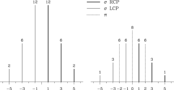
In the presence of a magnetic field, the degeneracy of magnetic sublevels of a molecule is broken due to the Zeeman effect. Zeeman splitting of the hydroxyl radical (OH) is often used to infer magnetic field strengths, both in masers (e.g., Davies et al., 1966) and in thermal gas (e.g., Turner & Verschuur, 1970). For the main-line, $F$-conserving transitions, the line splits into one $\pi$ component at the systemic velocity and two $\sigma$ components ($\sigma^{+}$ and $\sigma^{-}$) shifted in opposite senses with respect to the systemic velocity. For transitions in which $\Delta F=\pm 1$, such as the 1612 MHz ($F=1\rightarrow 2$) and 1720 MHz ($F=2\rightarrow 1$) transitions of OH, the splitting is more complicated (Figure 1). These ground-state satellite lines split into six $\sigma$ components ($\sigma^{\pm 1,2,3}$) and three $\pi$ components ($\pi^{0},\pi^{\pm}$), with component intensities in local thermodynamic equilibrium (LTE) being strongest for the innermost $\sigma^{\pm 1}$ components (Figure 2). Excited-state satellite lines split into a larger number of components; for instance, the 6016 and 6049 MHz lines each split into 15 different lines in the presence of a magnetic field (Davies, 1974).

With the exception of a single marginal Zeeman triplet at the $F$-conserving 1665 MHz transition in W75 N (Hutawarakorn et al., 2002; Fish & Reid, 2006), a full Zeeman pattern has never been observed in interstellar OH masers. In most sources, no clear $\pi$ components are seen at all. In the $F$-nonconserving satellite lines, theoretical considerations of cross-relaxation among magnetic sublevels due to trapped infrared radiation predict that even the $\sigma^{\pm 2}$ and $\sigma^{\pm 3}$ components should not be observable (Goldreich et al. 1973b as well as the discussion in Lo et al. 1975). Single-dish observations of the 1612 MHz OH transition in Orion A are suggestive of the presence of $\sigma^{\pm 2}$ and $\sigma^{\pm 3}$ components (Chaisson & Beichman, 1975; Hansen, 1982) but are not conclusive, since it is not clear that all spectral features come from the same spatial region. Nevertheless, the possibility that $\sigma^{\pm 2}$ and $\sigma^{\pm 3}$ components may exist in OH masers presents practical difficulties for observers of satellite-line transitions, as noted by Fish et al. (2003) and Hoffman et al. (2005a). Conversion of the velocity difference of $\sigma$ components in a Zeeman pair to a magnetic field strength is dependent upon the Zeeman splitting coefficient, which is different depending on which $\sigma$ components are seen. Traditionally it has been assumed that only the $\sigma^{\pm 1}$ components are seen, for which a Zeeman splitting of 0.654 kHz mG^-1 is appropriate at 1612 and 1720 MHz. But it is possible that several $\sigma$ components overlap for small Zeeman splittings, in which case the Zeeman splitting coefficient appropriate for conversion to a magnetic field strength may be a weighted average of the splitting coefficients of the $\sigma$ components. Indeed, comparison of magnetic fields obtained from Zeeman splitting of the 1720 MHz transition are often a factor of 1.5 to 2 higher than those obtained in the same spatial region at 1665 or 1667 MHz (Fish et al., 2003; Caswell, 2004), although Gray et al. (1992) do note an instance in W3(OH) in which the splitting between two 1720 MHz features of opposite polarization appears consistent with their interpretation as $\sigma^{\pm 1}$ components with a splitting coefficient (between $\sigma$ components) of 0.12 km s^-1 mG^-1. It has heretofore been unclear whether the Fish et al. and Caswell results indicate that 1720 MHz masers prefer higher densities (which are correlated with magnetic field strength) or that multiple $\sigma$ components from the same Zeeman group are blended together. It is interesting to note that the Zeeman splitting coefficient between a blend of all $\sigma^{+}$ and $\sigma^{-}$ components in their LTE ratio of intensities is exactly twice the splitting coefficient of the $\sigma^{+1}$ and $\sigma^{-1}$ components alone.

High spectral-resolution observations of OH masers are also important in order to determine the maser lineshapes. Theoretical models suggest that maser lineshapes may be sensitive to the degree of saturation and to the amount of velocity redistribution of molecules along the maser amplification path (Goldreich & Kwan, 1974; Field et al., 1994; Elitzur, 1998). While other masers have been observed at high spectral resolution, such as 12 GHz CH₃OH masers (Moscadelli et al., 2003) and 22 GHz H₂O masers (Vlemmings & van Langevelde, 2005), OH masers have never been observed with both the high spectral resolution required to determine the shape of the line wings and the high angular resolution required to ensure that spatially-separated maser spots are not blended together in the beam. The lack of such observations may be due to instrumental limitations. Since the velocity extent of OH maser emission in massive star-forming regions is typically several tens of km s^-1, an appropriately wide bandwidth is usually selected in order to observe all maser spots simultaneously. Because the number of spectral channels allowed by the correlator is generally limited (e.g., 1024 channels per baseband channel for the Socorro correlator, or only 128 channels in full-polarization mode), ground-state masers are usually observed at 1 kHz (0.18 km s^-1) resolution to within a factor of two.

It is in these interests that we have undertaken observations of OH masers in two high-mass star-forming regions at very high spectral resolution. Orion KL was chosen in order to examine whether the features observed by Hansen (1982) consist of a single Zeeman group or several spatially-unrelated maser features. W3(OH) was chosen because it is a frequently studied massive star-forming region with a well understood magnetic field structure (Bloemhof et al., 1992) and has several bright maser features at 1612 and 1720 MHz (Masheder et al., 1994; Argon et al., 2000; Wright et al., 2004b).

2. Observations

Figure 1.— Satellite-line Zeeman components for the 1612 MHz transition of OH, adapted from Hansen (1982). Because the Zeeman splitting is different for different $F$ levels, the $\sigma$ and $\pi$ components for an $F$-nonconserving transition are nondegenerate. In the presence of a magnetic field, a 1612 MHz line will split into six $\sigma$ components and three $\pi$ components. In the presence of a magnetic field along the line of sight, the $\sigma^{+}$ components are left circularly polarized and the $\sigma^{-}$ components are right circularly polarized. The Zeeman splitting for the 1720 MHz transition is analogous. Splittings are not to scale.

Figure 2.— Zeeman splitting pattern of 1612 and 1720 MHz masers in LTE, adapted from Davies (1974). Left: Splitting pattern when the magnetic field is along the line of sight. No $\pi$ components are present in the spectrum. Numbers above the lines indicate the relative intensities. Numbers along the axis indicate the velocity shift of the Zeeman components from the systemic velocity, in units of 0.061 km s^-1 mG^-1 for the 1612 MHz transition and 0.057 km s^-1 mG^-1 for the 1720 MHz transition. In the presence of a positive magnetic field (i.e., oriented in the hemisphere pointing away from the observer), the RCP $\sigma^{-}$ components are shifted to higher velocity than the LCP $\sigma^{+}$ components; a negative magnetic field produces the reverse pattern. Right: Splitting pattern when the magnetic field is nearly in the plane of the sky. Intensities of the $\sigma$ components are in the same ratio, though a factor of two weaker than for the case of the magnetic field along the line of sight. Three $\pi$ components also appear.

The National Radio Astronomy Observatory’s Very Long Baseline Array (VLBA) was used to observe the ground-state OH masers in two massive star-forming regions: W3(OH) and Orion KL. Data were collected starting at approximately 09 00 UT on 2005 September 20 using all 10 antennas. Approximately 2.3 hours of on-source observing time was devoted to W3(OH) and 1.0 hours to Orion KL. DA193 was also observed as a bandpass calibrator.

All four ground-state transitions (1612.23101, 1665.40184, 1667.35903, and 1720.52998 MHz) were observed in dual circular polarization. A bandwidth of 62.5 kHz was divided into 512 spectral channels with 122 Hz channel spacing (0.02 km s^-1 velocity spacing). The usable equivalent velocity bandwidth of about 10 km s^-1 was centered at $-44$ km s^-1 LSR for W3(OH) and $+10$ km s^-1 for Orion KL. Many OH maser spots fall outside this velocity range in Orion KL, but the bandwidth was centered appropriately to include the 1612 MHz maser feature at $+8$ km s^-1 for which Hansen (1982) claimed detection of $\sigma^{\pm 2}$ components. The data were sampled in 4-level (2-bit) mode. A correlator averaging time of 4 seconds was used. Due to the large oversampling required to record 62.5 kHz of bandwidth, 122 Hz is the highest spectral resolution available to the Socorro correlator. Four of the stations (Brewster, North Liberty, Owens Valley, and St. Croix) used the original VLBA tape-based recording system, while the other six used the newer Mark 5 disk-based recording system.

The data were reduced using the NRAO Astronomical Image Processing System (AIPS). Left circular polarization (LCP) data from the North Liberty station were unusable due to anomalously low amplifier gain. Data from the Hancock station were discarded due to strong radio frequency interference (RFI). Weaker RFI contaminated some data from other stations as well. An auto-correlation bandpass was applied to the data (for further details see §3.3). Each of the four maser transition frequencies was self-calibrated and imaged separately. Additionally, the left and right circular polarizations were self-calibrated and imaged separately from each other in the 1665 and 1667 MHz transitions, due to RFI that affected each polarization differently. No polarization calibration was applied, as the VLBA polarization leakage is small enough for our scientific purposes. Image cubes were created in both circular polarizations. Each velocity channel was searched for maser emission, and one or more elliptical Gaussians were fitted to detected features using the fitting routines of the AIPS task JMFIT.

3. Results

Figure 3.— Ground-state OH masers in W3(OH). Symbols indicate maser spots as follows: plus signs, 1665 MHz; diamonds, 1667 MHz; triangles, 1612 MHz; squares, 1720 MHz.

The detected spots are listed in Table 1 and shown in Figure 3. Symbols are plotted at the locations of peak emission both in LCP and in RCP (right circular polarization). Alignment of maser maps at different frequencies was accomplished by comparison with the data of Wright et al. (2004b). We estimate that resulting relative positional errors between frequencies is $\sim 10$ mas, due partly to errors in estimating spot positions in the two epochs and partly to the inherent motion of the maser spots. Maser proper motions in W3(OH) are about 3 to 5 km s^-1 (Bloemhof et al., 1992), which corresponds to 3 to 5 mas in the 9-year baseline between the Wright et al. (2004a, b) observations and the present data. Zeeman pairs are identified in Table 2.

Our map is qualitatively similar to the Wright et al. (2004b) map. We recover the vast majority of maser spots in their data. Omissions may be explained by the difference in sensitivity in the observations. The Wright et al. (2004a, b) observations spent nearly a factor of 5 more time on source with a factor of 4 coarser velocity resolution. Additionally, data from the Hancock and (frequently) North Liberty VLBA stations were not usable in the present observations, further reducing our sensitivity.

We were unable to detect any satellite-line maser emission in Orion KL. Our pointing center was chosen to be 4″ to the northeast of the group marked “Center” in the map of Johnston et al. (1989), which is the probable location of the Stokes V spectrum interpreted as a 4-component Zeeman pattern centered at velocity 8.0 km s^-1 by Hansen (1982). At this pointing center, peak amplitude loss to time-average smearing is small (5% at 7″). Bandwidth smearing is negligible with our extremely narrow spectral channels. The nondetection is therefore likely due to a decrease in the flux density of the 8 km s^-1 1612 MHz features in the 20 years since the Johnston et al. observations. (Note that their measured flux densities are lower than those of Hansen seven years prior.) Because our primary goal in these observations was to address the issue of satellite-line Zeeman splitting and the Orion KL main-line data were of inferior quality to the W3(OH) data, the Orion KL data were not further analyzed.

3.1. Lineshapes and Gaussian Components

Figure 4.— Spectra of selected features with a near Gaussian lineshape. The top portion of each panel shows the data and best Gaussian fit. The bottom portion shows the residuals. Spot numbers as listed in Table 1 are indicated for each panel. The top, middle, and bottom rows show spectra fitted with one, two, and three Gaussian components, respectively.

Figure 5.— Top: Normalized deviation from Gaussian shape for near-Gaussian maser features with peak intensity brighter than 1 Jy beam^-1. Bottom: FWHM as a function of peak intensity. Masers in the 1665 MHz transition (bolded) appear to have a wider spectral profile than masers in the other ground state transitions.

Figure 6.— Map of spots included in analysis of lineshapes. Circled symbols indicate maser spots with fitted FWHM greater than 0.227 km s^-1; bolded symbols indicate maser spots with FWHM greater than 0.30 km s^-1.

Even at this high spectral resolution, the OH maser spectral profiles can usually be fitted well with one or a small number of Gaussian components in the spectral domain. The top panels in Figure 4 show selected maser spots with single-Gaussian fits. For spots weaker than $\sim 1$ Jy beam^-1 (about half the spots), a single Gaussian component usually fits the spectral profile due to signal-to-noise limitations. For spots with a larger signal-to-noise ratio, more complicated spectral profiles are seen as well. Some maser profiles appear skewed or have asymmetric tails. For the most part, these can be fairly well fitted by two or three Gaussian components, as shown in the middle and bottom panels of Figure 4. In some instances, two or more maser lines at different velocities may appear at approximately the same spatial location. When multiple distinct peaks are present in the spectral domain at the same spatial location, we identify each peak as maser line for purposes of inclusion in Table 1. It is observationally cleanest to identify these as separate features, although theoretical models indicate that under certain conditions the spectrum of a single masing spot could be multiply peaked (e.g., Nedoluha & Watson, 1988; Field et al., 1994).

The normalized deviation ($\delta$) of a lineshape from a Gaussian shape can be defined by

$$\delta=\frac{\int\left[I(v)-a_{1}\exp(-v^{2}/a_{2})\right]^{2}\,dv}{I_{p}^{2}\,\Delta v},$$

where $I(v)$ is the intensity distribution as a function of velocity, $a_{1}$ and $a_{2}$ are parameters from the best Gaussian fit, $I_{p}$ is the peak intensity, and $\Delta v$ is the FWHM of the distribution (Watson et al., 2002). Figure 5 shows the distribution of $\delta$ (calculated over the entire range of channels in which the maser spot is detected) and the FWHM as a function of $I_{p}$ for masers with a peak intensity greater than 1 Jy beam^-1. Excluded from consideration are masers with multiple peaks or extended asymmetric tails (e.g., with profiles as in the bottom of Figure 4) as well as maser features for which spatial blending with a second maser feature within the beam prohibits accurate determination of the spectral profiles of the two features individually.

Derived values of $\delta$ range from 0 to $6\times 10^{-3}$, consistent with theoretical predictions by Watson & Wyld (2003). The distribution is suggestive of a fall-off of $\delta$ for large values of $I_{p}$, but with only five data points having $I_{p}>30$ Jy beam^-1, this result is not statistically significant. Watson & Wyld predict that $\delta$ attains a maximal value when the stimulated emission rate, $R$, is a few times the pump loss rate, $\Gamma$, and then decreases with increasing $R/\Gamma$ (i.e., as the maser becomes increasingly saturated). Their model also predicts that when $R/\Gamma$ is large enough for $\delta$ to decrease noticeably, the line profile should rebroaden to nearly the thermal Doppler linewidth. In our observations, the FWHM linewidth of maser spots has a range of 0.15 to 0.38 km s^-1 and is independent of the peak intensity of the maser spot. This suggests that even the brightest masers in a typical star-forming region (which are clearly saturated) may not be sufficiently saturated to exhibit rebroadening.

The FWHM linewidth does appear to be a function of maser transition. As shown in Figure 5, 1665 MHz masers are on average broader than their other ground-state counterparts. The mean and sample standard deviation of the FWHM are $0.244\pm 0.058$ km s^-1 for the 1665 MHz transition and $0.192\pm 0.025$ km s^-1 for the other three transitions combined. Sixteen of the 28 1665 MHz masers brighter than 1 Jy beam^-1 are broader than 0.227 km s^-1, the linewidth of the broadest maser in any of the other three transitions. The spatial distribution of masers meeting the brightness and shape criteria for the above analysis is shown in Figure 6. As can be seen by comparison with Figure 3, nearly all of the broad 1665 MHz maser spots appear in regions where no ground-state OH masers are found except in the 1665 MHz transition. The only broad 1665 MHz masers found in proximity to masers of other ground-state transitions are in the cluster of masers near the origin. This region is notable for the existence of highly-excited OH (Baudry et al., 1993; Baudry & Diamond, 1998) and is presumed to mark the location of an O-type star exciting the H II region. As such, it is likely that the physical conditions change in this region over a shorter linear scale than in other regions of W3(OH).

3.2. Satellite-Line Splitting

Figure 7.— Fits of the brightest 1720 MHz Zeeman pair in W3(OH). Top: Best three-component fit to each polarization. LCP emission is shown in red and RCP in blue. The individual fit components are shown as dotted lines, and the total fit spectra are shown as solid lines. Residuals are shown below the fits. Bottom: Best six-component fit constraining the center velocities of each component to be spaced as in Figure 2. Note that the pattern of intensities (in yellow) is not symmetric about a center velocity for the $\sigma^{+}$ and $\sigma^{-}$ components. The significantly poorer fit does not justify the reduction in the number of parameters.

Figure 8.— Spectra of satellite-line Zeeman pairs. LCP emission is shown in red and RCP in blue. Gaussian fits are superposed in solid lines; individual Gaussian components are shown in dotted lines. The top right and top left panels exhibit complicated lineshapes, the latter due to blending of several components within the beam. However, there is no evidence for $\sigma^{\pm 2,3}$ components.

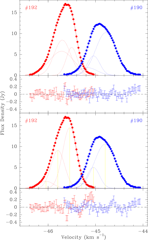
There is no evidence of the presence of multiple $\sigma$ components in the single-polarization spectra of the satellite-line (1612 and 1720 MHz) transitions. We find four Zeeman pairs at 1720 MHz and seven at 1612 MHz. Figure 7 shows the LCP and RCP spectra of the brightest 1720 MHz Zeeman pair. The top panels show the best three-component fit to each polarization. The residuals suggest that a fourth, weak component may be required to fit the high-velocity tail of RCP emission. The magnetic field strength derived from applying the splitting coefficient appropriate for $\sigma^{\pm 1}$ components to the velocities of the peak channels of emission in spots 190 and 192 is $+6.6$ mG.

The velocities of the two strongest, narrow Gaussian components in each circular polarization in the top panels of Figure 7 are consistent with a 2:1 splitting ratio centered at approximately $-45.26$ km s^-1 to within the errors in determining the center velocities of the Gaussians. The only lines in a symmetric, incomplete Zeeman pattern with this ratio are the $\sigma^{\pm 1}$ and $\pi^{\pm}$ components. Nevertheless, we reject the possibility that the two brightest Gaussians correspond to $\pi$ components for several reasons. First, they are only seen in one circular polarization, while $\pi$ components should be 100% linearly polarized (although see Fish & Reid 2006 for a discussion of the possibility of $\pi$ components with nonzero circular polarization fractions). Second, the $\pi^{0}$ component is missing from this pattern, although theory predicts that it should be stronger than $\pi^{\pm}$ components. Third, no other $\pi$ components are seen in the ground-state masers in W3(OH) (García-Barreto et al., 1988). Linear polarization is rare in W3(OH); all masers are more circularly polarized than linearly polarized.

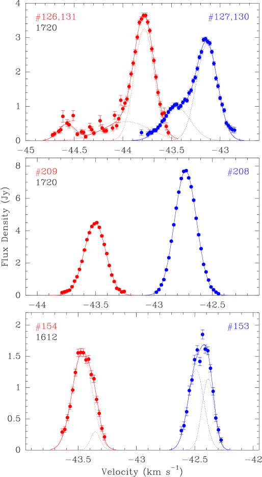
The bottom panels show the best fit constraining the center velocities of each component to be in the ratio expected from the Zeeman pattern of multiple $\sigma$ components in each polarization, as shown in Figure 2. It is not the case that the two Gaussian components closest to the systemic velocity are brightest. This argues against interpretation of the spectra as $\sigma^{\pm 1,2,3}$ components in their LTE ratios. It is more probable that the same factors that produce asymmetric, non-Gaussian lineshapes in the main-line transitions (as in the middle and bottom panels of Figures 4) also produce non-Gaussian asymmetries in the $\sigma^{\pm 1}$ components at 1720 MHz. Indeed, at higher angular resolution, Masheder et al. (1994) note that features 190 and 192 are each actually a cluster of several maser spots. This is consistent with the increasing intensities in each polarization toward higher velocity, suggesting that our observed features may be the result of blending of (at least) three nearby Zeeman pairs with a regular shift in velocity but approximately the same magnetic field (coincidentally also $+6.6$ mG if interpreted as $\sigma^{\pm 1}$ components). This magnetic field value is consistent with the two nearby Zeeman pairs to the northeast: $+6.4$ mG from spots 212 and 218 at 1665 MHz and $+6.8$ mG from spots 208 and 209 at 1720 MHz. (Note that this latter Zeeman pair, shown in the middle panel of Figure 8, is unquestionably comprised solely of $\sigma^{\pm 1}$ components, since there is only one feature in each circular polarization and interpretation of these features as $\sigma^{\pm 2}$ components would imply a magnetic field strength of $+2.2$ mG, a value too small to be consistent with the 1665 MHz magnetic field or any other magnetic field strength in the cluster of maser spots near the origin.)

Figure 8 shows the LCP and RCP spectra of the other two 1720 MHz Zeeman pairs and one 1612 MHz Zeeman pair in W3(OH). The multiple peaks in the single-polarization spectra of the top panel are again due to blending of two adjacent maser spots. It is clear that these are not due to spatially-shifted $\sigma^{\pm 2,3}$ components from a single Zeeman pattern, since the spectra are not symmetric by reflection across a single, systemic velocity. We interpret the spectra as two Zeeman pairs, each with a different magnetic field strength. Asymmetric amplification of the various peaks in LCP and RCP may also be partly due to the large velocity range spanned — greater than 1.4 km s^-1 from the low-velocity peak in LCP to the high-velocity peak in RCP. Since this is more than twice the turbulent velocity dispersion of a maser cluster in W3(OH) (Reid et al., 1980), it would be expected that the emission from multiple maser spots in this velocity range might be amplified by different amounts.

The middle panel in Figure 8 shows a 1720 MHz Zeeman pair that is well fitted by a single Gaussian component in each polarization. The bottom shows a 1612 MHz Zeeman pair. It is clear from the velocities of the fit components that the lines are not produced from multiple $\sigma$ components of a single Zeeman pattern. Emission from other masers in the 1612 MHz transition is qualitatively similar to these Zeeman pairs. The image cubes of 1612 and 1720 MHz emission were searched thoroughly at the locations of the detected masers for indications of weak emission at other velocities. No emission was detected to within the limits of our noise except as listed in Table 1.

3.3. Positional Gradients

Figure 9.— Positional gradients as a function of LSR velocity for a selection of maser spots. Boxes are 20 mas on a side. The position in each velocity channel is represented as an ellipse one-tenth the size of the undeconvolved spot size, fit as an elliptical Gaussian. The black contour denotes the channel of peak emission; colors indicate velocity-shifted channels. Dotted contours indicate channels in which the SNR is less than 10. Panels a through j show the gradients in ten Zeeman pairs. Boxes are aligned separately for the RCP (always on top) and LCP (bottom) data. The gradients of the RCP and LCP components of the three Zeeman pairs at 1720 MHz are similar in amplitude and well aligned in position angle. Panels k through o show additional interesting spots. The velocity gradient measured in km s^-1 mas^-1 is inversely proportional to the positional gradient (presented here) measured in mas (km s^-1)^-1.

Figure 10.— Map of velocity gradients of spots with peak brightness greater than 1 Jy beam^-1. Arrows point in the direction of change with increasing line-of-sight velocity. Velocity gradients are generally large in the cluster near the origin and smaller elsewhere.

Figure 11.— Velocity gradients and position angle differences of those velocity gradients for components of Zeeman pairs (circled) and echoes (not circled; defined in §3.3). Error bars are shown along the abscissa only. The magnitude of the velocity gradient is determined by taking the inverse of the average of the positional gradients as measured in mas (km s^-1)^-1 of the RCP and LCP components. Dotted lines indicate RCP$-$LCP position angle differences of $\pm$45°. In most Zeeman pairs, LCP and RCP gradients are roughly aligned. This is especially true for the three 1720 MHz Zeeman pairs.

Figure 12.— Magnitude of velocity gradient as a function of peak brightness. There does not appear to be a correlation between the velocity gradient and maser brightness. However, of the 22 1667 MHz maser spots for which a gradient is determined (displayed in bold for contrast), the largest gradient is 0.14 km s^-1 mas^-1.

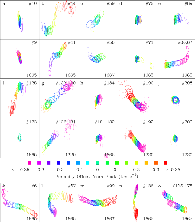
In general, the position of a maser spot is seen to vary across the linewidth (e.g., Moscadelli et al., 2003; Hoffman et al., 2003). Figure 9 shows the maser position as a function of LSR velocity for a sample of maser spots. The position of the center of the best-fitting elliptical Gaussian usually varies linearly as a function of velocity. In some instances the position may trace out a curving structure rather than a straight line, but all maser spots display organization in their position as a function of frequency.

Table 1 includes the velocity gradient and position angle (degrees east of north) in the direction of increasing velocity for each maser spot. The velocity gradients were determined algorithmically. On both sides of the peak, the nearest channel with emission below half of the peak brightness was identified. The velocity difference between these two channels was divided by the difference in positions. For a Gaussian spectral profile this corresponds to dividing the FWHM by the difference of the positions across the FWHM, but it is algorithmically implementable for any emission spectrum, including spectra with multiple peaks, as in the middle and bottom panels of Figure 4. For consistency with Moscadelli et al. (2003), we report the velocity gradients in units of km s^-1 mas^-1 rather than the positional gradient in mas (km s^-1)^-1. A large positional gradient corresponds to a small velocity gradient, and vice versa.

These gradients appear to be real, not an artifact due to residual calibration or bandpass phase errors. Comparison of selected bright maser spots in different regions of W3(OH) indicate that positional gradients determined from applying the auto-correlation (real) bandpass are consistent with those determined from applying the cross-correlations (complex) bandpass to within measurement errors. Since the auto-correlation bandpass has a higher signal-to-noise ratio and the phases of the cross-correlation bandpass are constant with frequency over the region of interest, the auto-correlation bandpass was applied. In addition, combinations of plots of the Right Ascension or Declination positional gradients versus Right Ascension offset, Declination offset, or LSR velocity are all consistent with a random scatter about zero (as with Figure 6 in Moscadelli et al.), both for individual transitions and polarizations as well as for the ensemble of all maser spots with detected positional gradients as listed in Table 1. However, the two-dimensional distribution does show larger velocity gradients (smaller positional gradients) near the origin (Figure 10). Note that the origin is not near the location of the reference spots for self-calibration except at 1720 MHz and the LCP polarization at 1665 MHz, nor is it near the pointing and correlation center (taken from Argon et al., 2000), which is at $(\Delta\alpha,\Delta\delta)\approx(-884,+311)$ mas.

It is probable that some gradients are the result of two maser spots within a beamwidth that blend together spectrally. One clear instance of this is shown in the top panel of Figure 8. Only one feature is detected in each circular polarization in each spectral channel. Yet it is clear from the spectra that there are at least two distinct maser spots in each polarization. The weaker peak is to the northwest of the strong peak (panel g of Figure 9). The centroid of the fitted Gaussian is effectively a weighted average of the two positions at velocities intermediate to the two peak velocities. This effect is more prominent in RCP due to the smaller velocity offset between the two peaks. Nevertheless, there is a real positional gradient associated with each of the maser spots as well, as is clearest in the uncontaminated blue wing of the bright features.

Velocity gradients of the RCP and LCP components of a Zeeman pair are generally aligned. Figure 11 shows the distribution of position angle differences between the velocity gradients of the RCP and LCP components of Zeeman pairs. These position angle differences are also shown for “echoes,” i.e., spectral features detected in the opposite circular polarization and same location and line-of-sight velocity as another strong, partially linearly polarized spectral feature due to the fact that both circular feeds of a telescope are sensitive to linear polarization. These detections are not a result of telescope polarization leakage; in most cases, the brightness of the weaker polarization feature is more than 25% of that of the stronger polarization feature, while polarization leakage of the VLBA feeds is only 2 to 3% (Wrobel & Ulvestad, 2005). Since an echo is a second, weaker detection of a single maser spot, both a maser spot and its echo would be expected to have essentially the same gradient. We find this to be the case; for the 9 maser spots for which a gradient can be determined algorithmically both for itself and its echo, all have gradient polarization angle differences less than 40°. Of the 23 Zeeman pairs for which gradients can be obtained for both components, the RCP and LCP components are aligned to within better than 45° for 18 of them. Larger deviations for the other pairs can usually be attributed to spatial blending with nearby maser spots. The alignment of RCP and LCP gradients is especially pronounced in the bright Zeeman pairs at 1720 MHz. Their spectra and positions are shown in Figures 7, 8, and 9. In each case, there is a clear, linear positional gradient that is similar for both components of the Zeeman pair.

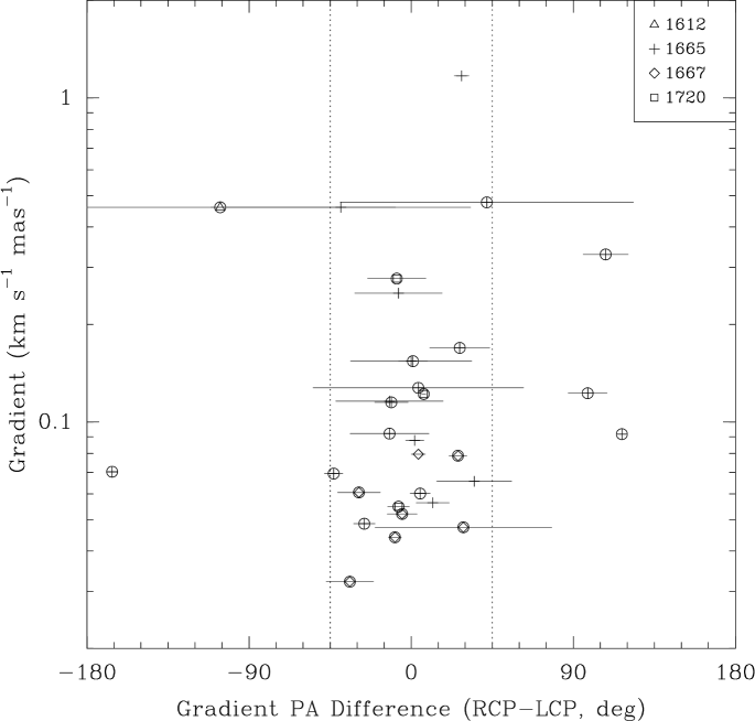
The magnitude of the velocity gradient of a maser spot does not display a clear correlation with its peak brightness, as shown in Figure 12. However, there does appear to be an absence of 1667 MHz maser spots with large velocity gradients. (That is, 1667 MHz masers appear to have large positional gradients as a function of line-of-sight velocity.) This is consistent with observations by Ramachandran et al. (2006). It is unclear whether the line-of-sight velocity gradient projected onto the plane of the sky necessarily allows inference of the line-of-sight velocity gradient along the amplification path. Large velocity gradients along the amplification length may destroy the velocity coherence required for significant amplification, so the population of detectable maser spots may have an inherent bias in favor of areas where the projection of the velocity gradient along the line of sight is small. But in §4.2 we present further evidence that the velocity gradient along the amplification path is indeed small in 1667 MHz masers.

There does not appear to exist a correlation between the orientation of the gradient of a maser spot and its proper motion vector. From the list of 1665 MHz maser spots for which Bloemhof et al. (1992) were able to measure a proper motion, approximately three dozen spots with measurable positional gradients were recovered in our observations. Since the Bloemhof et al. data were not phase referenced, multiple reference frames consisting of their proper motions with an added constant vector were compared against our positional gradient vectors. No clear correlations were found. Proper motion maps of the OH masers in W3(OH) display a clear large-scale pattern of motions (Bloemhof et al., 1992; Wright et al., 2004a), while the map of gradients shows no such large-scale organization, with the possible exception of the cluster near the origin (Figure 10), where velocity gradients are large (i.e., positional gradients are small). If there is a connection between observed maser velocity gradients and material motions, it is probable that it is the turbulent motions that dominate, not the large-scale organized motions.

Likewise, the gradients do not correlate with linear polarization fraction (which is zero for most maser spots) or polarization position angle, as determined from García-Barreto et al. (1988). The magnetic field direction can theoretically be derived from the linear polarization fraction and position angle (e.g., Goldreich et al., 1973a), although empirical data suggest that recovery of the full, three-dimensional orientation of the magnetic field may not actually be possible at OH maser sites (Fish & Reid, 2006).

3.4. Deconvolved Sizes and Maser Geometry

Figure 13.— Deconvolved spot sizes as a function of velocity for selected maser spots, identified by spot number and transition. The geometric mean of the deconvolved major and minor axes is plotted as a function of velocity offset from the channel of peak flux density. Dots represent the nominal deconvolved spot size, while the lines represent the allowed range of values within the noise. Grey, dotted lines represent measurements with an SNR of less than 10.

The apparent size of a maser may be a function of frequency offset from line center, due to saturation effects dependent on the maser geometry. For example, Elitzur (1990) calculates that the size of a spherical maser should increase exponentially with $|\nu-\nu_{0}|/\Delta\nu_{\mathrm{D}}$, where $\nu_{0}$ is the line center frequency and $\Delta\nu_{\mathrm{D}}$ is the Doppler linewidth. This effect can be large; Elitzur calculates that the apparent spot size at half the Doppler width may be twice that at line center (peak flux).

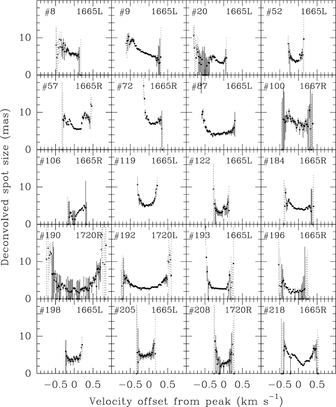
Figure 13 shows deconvolved spot sizes as a function of velocity offset from the channel of peak emission for 20 selected maser spots. Displayed masers were selected under the criteria that they have a peak flux density of at least 7 Jy and not have obvious spatial blending with other maser emission. Minimum nominal deconvolved spot sizes typically range from 3 to 6 mas, consistent with results obtained for 1665 MHz masers by García-Barreto et al. (1988), although the apparent sizes of 1720 MHz masers are much bigger than the $\leq 1.2$ mas upper limit obtained by Masheder et al. (1994) (see §3.2 for discussion of probable spatial blending in spot numbers 190 and 192). In general, maser spot sizes appear to increase toward the line wings, although the degree to which the spot size increases with frequency offset from center (or indeed whether it does at all) is different with each maser spot. In some spots, the spot size is a complicated function of frequency. It is possible that some maser spots display additional structure on scales smaller than the beam size, which could cause the spot size to be overestimated over part or all of the line profile. In any case, the variation of spot size over the observable line profile is sufficiently small and variable to preclude accurate determination of the functional form of the apparent spot size as a function of frequency (and therefore geometry).

The velocity offset at which the maser spot size doubles is generally greater than 0.5 km s^-1. For a spherical maser, this implies a Doppler width greater than 1.0 km s^-1, based on the Elitzur (1990) model, which would require a kinetic temperature in excess of 400 K. This value is more than a factor of two higher than the inferred effective temperature of the ambient radiation field (Walmsley et al., 1986). It is probable that the geometry of the OH masers in W3(OH) is not spherical. Other theoretical considerations lead Goldreich & Keeley (1972) to conclude that a filamentary geometry is more typical of astrophysical masers. Alternatively, several different (spherical) clumps may overlap along the line of sight to produce a detectable maser.

4. Discussion

4.1. $\sigma$ Components in Satellite-Line Transitions

We find no evidence of the presence of $\sigma^{\pm 2,3}$ components in the 1612 and 1720 MHz satellite lines of OH. Some of the spectral profiles in the 1720 MHz transition appear to consist of several Gaussian components (Figures 7 and 8), but the velocities and intensities of these components are not consistent with what is expected by theory (Figure 2). The nondetection of $\sigma^{\pm 2,3}$ components lends support to the prediction that cross-relaxation across magnetic sublevels will favor amplification of the $\sigma^{\pm 1}$ components over the other $\sigma$ components (Goldreich et al., 1973b). For the brightest 1720 MHz maser, our nondetection of accompanying maser components requires that $S_{\sigma^{\pm 1}}/S_{\sigma^{\pm 2}}>$ a few hundred. Future observations of sources with stronger satellite-line OH maser emission, such as G43.165$-$0.028 (Argon et al., 2000) and G331.512$-$0.103 (Caswell, 1999), could improve on this by more than a factor of 10.

Could $\sigma^{\pm 2}$ components ever be observed in a maser source? The number of gain lengths for a $\sigma^{\pm 1}$ component will be twice that of a $\sigma^{\pm 2}$ component over the same physical region of space. For unsaturated amplification, the intensity depends exponentially on the number of gain lengths, effectively prohibiting detection of the $\sigma^{\pm 2}$ components. (Since the number of gain lengths for the $\sigma^{\pm 1}$ components is $\gtrsim 20$ (Goldreich et al., 1973b), the $\sigma^{\pm 2}$ components would be weaker by a factor of $\gtrsim e^{10}$). If the $\sigma^{\pm 1}$ components are highly saturated, it is possible that the $\sigma^{\pm 2}$ components would be detectable, provided that the populations of the magnetic sublevels are not redistributed by radiative transitions connecting these levels with the far infrared. It should be noted that two different radiative effects are likely operating in satellite-line masers. First, cross-relaxation of the magnetic sublevel populations due to radiative transitions connecting these levels with the far infrared will favor the $\sigma^{\pm 1}$ components (Goldreich et al., 1973b). This effect can operate over frequency differences much greater than the linewidth of a single maser component. Second, velocity redistribution inherent in a three-dimensional geometry causes maser lines to remain narrow even during saturation, preventing rebroadening to the Doppler width (Field et al., 1994). Velocity redistribution causes flux from the linewings to move toward the line center, effectively changing the frequency on the order of a maser linewidth. Cross-relaxation of populations of the magnetic sublevels will be unavoidable in regions of strong infrared radiation. Thus, it is probable that $\sigma^{\pm 2}$ components will not be detectable in massive star-forming regions.

It is also likely that 1720 MHz supernova remnant masers will not display evidence of $\sigma^{\pm 2}$ components. Supernova remnant OH masers are collisionally pumped (Elitzur, 1976; Frail et al., 1994), so it may be possible to avoid far infrared cross-relaxation among magnetic sublevels. However, the Zeeman splitting is usually less than the maser linewidth (e.g., Hoffman et al., 2005a, b), resulting in blending of multiple maser components into a single maser line. Velocity redistribution would likely destroy the signature of $\sigma^{\pm 2,3}$ components, if emission in these modes is produced.

As mentioned in §1, if $\sigma^{\pm 2,3}$ components are not blended with $\sigma^{\pm 1}$ components at 1720 MHz, there is observational evidence that the magnetic field, and hence the density, at sites of 1720 MHz maser emission in massive star-forming regions may be higher than at sites of 1665 and 1667 MHz maser emission (Fish et al., 2003; Caswell, 2004). Our data indicate that $\sigma^{\pm 2,3}$ components, if they exist, are so weak as to have no effect on the observed emission. Thus, the value of the magnetic field obtained from assuming a Zeeman splitting coefficient appropriate for pure $\sigma^{\pm 1}$ components is reliable. Using this coefficient, the three brightest 1720 MHz Zeeman pairs in W3(OH) are consistent with the magnetic field strengths derived from nearby main-line Zeeman pairs. Models of Pavlakis & Kylafis (1996) suggest that 1720 MHz maser activity may be favored at densities near or just above those for which 1665 MHz maser activity occurs. Thus, in an ensemble of OH maser sources, it would be expected that the magnetic fields derived from 1720 MHz Zeeman splitting would be skewed higher than those obtained at 1665 MHz (consistent with the findings of Fish et al. 2003 and Caswell 2004) , although the magnetic field strengths derived at 1665 MHz and 1720 MHz would be similar in some of those sources (consistent with this work).

4.2. Comparison of Maser Transitions

Our results for the properties of hydroxyl masers at high spectral resolution are remarkably similar to those found in a similar study of 12.2 GHz methanol masers in W3(OH) (Moscadelli et al., 2003). FWHM line widths of single-Gaussian fits range from 0.15 to 0.38 km s^-1 in OH, as compared with the range 0.14 to 0.32 km s^-1 in CH₃OH. Normalized deviations from a Gaussian shape are several $\times 10^{-3}$ for both the OH and CH₃OH masers. Gradients in the spot position as a function of velocity are observed in both species, with similar amplitudes. The OH masers in our sample have velocity gradients as a function of position (i.e., the inverse of a positional gradient as a function of line-of-sight velocity) of 0.01 to 1 km s^-1 AU^-1 (with one outlier at 5 km s^-1 AU^-1), as compared to 0.02 to 0.30 km s^-1 AU^-1 in a smaller sample of CH₃OH masers (Moscadelli et al., 2003). The similar observational characteristics of OH and CH₃OH masers are not surprising given that these molecules form in the same environment (Hartquist et al., 1995), are both excited under similar conditions (Cragg et al., 2002), and appear in close proximity (Etoka et al., 2005).

Since the ground-state transitions of OH have large Zeeman splitting coefficients, an apparent velocity gradient could be the result of a magnetic field gradient. Indeed, in the cluster of maser spots located near the origin in Figure 3, the line-of-sight velocity gradients as a function of position are large, and the magnetic field strengths are large and change significantly on a small spatial scale (see Table 2 of the present work as well as Figure 13 of Wright et al., 2004b). Likewise, the velocity gradients are small in the cluster of masers near $(\Delta\alpha,\Delta\delta)=(-800,-700)$ mas, where the magnetic field strengths are small and the gradient of the magnetic field as a function of position is small. But the observed velocity gradients cannot be entirely due to magnetic field gradients, since they are also observed in methanol masers (Moscadelli et al., 2003), in which Zeeman splitting is negligible.

In the absence of velocity redistribution between velocity subgroups in the masing region, the linewidth of a saturated maser will in general increase as the amplification (and hence, intensity) of the maser increases (Goldreich & Kwan, 1974), although maser linewidths remain narrow even during saturated amplification when trapped infrared radiation is included in the theory. The lack of single-Gaussian lineshapes with FWHM greater than 0.4 km s^-1 combined with the absence of a correlation between FWHM linewidth and maser flux density suggests that line rebroadening does not occur, even for the brightest OH masers. Field et al. (1994) suggest that velocity redistribution is important at 1665 MHz, which would produce narrow, single-peaked maser lines, as observed. In extreme cases, increasing amplification may cause the line center to go into absorption, resulting in two very narrow maser lines at different velocities (Gray et al., 1991; Field et al., 1994). The addition of a velocity gradient over the amplification length can also produce very strong, leptokurtic intensity profiles. However, large velocity gradients in the presence of complete velocity redistribution can also produce multiply-peaked spectral profiles, which we do not observe. While spectral profiles do sometimes exhibit more than one peak (as in Figure 4), it is neither the case that the individual peaks in the spectrum are abnormally narrow nor that the overall spectrum resembles a single broad Gaussian whose center is strongly absorbed. It is more probable that these spectra are indicative of two or more spatially distinct maser spots blended within a beamwidth. VLBI studies of other sources find that it is common for several distinct maser spots to be found within several milliarcseconds of each other (e.g., Slysh et al., 2001; Fish et al., 2005).

We find that the linewidths of 1665 MHz masers are greater than the other ground-state OH masers. While 1665 MHz masers are usually the brightest OH masers in a source, the lack of a correlation between the linewidth and maser intensity indicates that saturated rebroadening is not the cause of the larger linewidths at 1665 MHz. One possible explanation may involve the large Zeeman splitting coefficient at 1665 MHz. A magnetic field gradient of 0.34 mG is sufficient to shift the center velocity of a 1665 MHz maser by the 0.2 km s^-1 FWHM typical in other transitions; necessary magnetic fields for similar shifts are 0.56 mG at 1667 MHz and over 1.6 mG in the satellite-line transitions. Observations of a larger sample of interstellar maser sources suggest that the magnetic field strength typically varies by a few tenths to a full milligauss in a typical cluster (projected dimension of several $\times 10^{15}$ cm) of maser spots (Fish & Reid, 2006). Since the amplification length (along the line of sight) is likely a factor of a few smaller than the clustering scale, it is reasonable that the magnetic field strength may change by a few tenths of a milligauss over the amplification length. If so, and if velocity redistribution is not total, it is possible that the resulting spectral profile would be broader. Under these assumptions, it would be expected that broader 1665 MHz masers would appear in regions where the gradient of the magnetic field is large. The central cluster does contain several broad 1665 MHz maser spots, and it is clear that the magnetic field strength varies significantly over a small spatial scale in this region. However, the other broad OH masers in W3(OH) appear in regions where the magnetic field strength is sampled (in this study and in Wright et al. 2004a, b) by only one or a few Zeeman pairs, so it is difficult to obtain an estimate of the gradient of the magnetic field in these locations. Indeed, since regions of large magnetic field gradients may not favor amplification of both $\sigma$-components in a Zeeman pair (Cook, 1966), it is possible that the magnetic field gradients in these regions are large.

A related possiblity is that the broad 1665 MHz masers sample a region of parameter space in which amplification of only the 1665 MHz masers is favored. Due to Zeeman splitting, a large magnetic field gradient might be expected to act akin to a large velocity gradient, although rigorous theoretical examination of the effect of magnetic field gradients in maser sites is lacking. With the exception of the central cluster of maser spots, in which physical conditions likely change substantially over a small spatial scale, all other broad 1665 MHz masers appear in regions where the only ground-state OH masers found are 1665 MHz masers. Models by Pavlakis & Kylafis (1996) indicate that for radiatively-pumped OH masers, amplification of 1667 MHz decreases significantly as the velocity gradient over the amplification path increases from 1 km s^-1 to 2 km s^-1, while 1665 MHz maser amplification remains relatively unaffected. This is in excellent qualitative agreement with Gray et al. (1992), who find that amplification of the 1667 MHz transition falls off with increasing velocity shift. In our observations, no broad 1665 MHz maser is found in the vicinity of 1667 MHz masers; in fact, 1667 MHz masers are the only ground-state transition absent from the highly active central cluster of masers. These facts fit well with the observation that 1667 MHz masers have small line-of-sight velocity gradients in the plane of the sky (see Figure 12), suggesting that the gradient of the line-of-sight velocity along the amplification path may be small as well.

It should be noted that the central cluster of masers also includes a 4765 MHz maser (Gray et al., 2001), for which inversion requires a small velocity gradient (Pavlakis & Kylafis, 1996). However, this maser is near the southern edge of the cluster (Etoka et al., 2005), where the magnetic field gradient is small. It may be the case that even in clusters with large velocity gradients, subregions exist in which the velocity gradient along the line of sight is small. In any case, it is not yet established whether gradients in the centroid of a maser spot as a function of line-of-sight velocity also provide information as to the line-of-sight velocity distribution along the amplification path of a maser spot. If maser amplification is only favored for a narrow range of velocity gradients along the amplification path, an unavoidable observational bias will exist. But velocity redistribution may weaken the correlation between velocity gradients and maser gain. Further theoretical and observational work may be required to resolve these issues.

5. Conclusions

We have observed over 250 ground-state OH maser spots at very high spectral resolution. Spectral profiles are generally well fit by one or a small number of Gaussian components. The data hint that deviations from Gaussianity may diminish for bright ($>30$ Jy) masers, but our sample size of bright masers is too small to be conclusive. Maser FWHM linewidths range from 0.15 to 0.38 km s^-1, with 1665 MHz masers generally having broader profiles than other ground-state masers.

Consistent with theoretical predictions (Goldreich et al., 1973b), we do not see $\sigma^{\pm 2,3}$ components in the 1612 and 1720 MHz satellite-line transitions. When satellite-line Zeeman pairs are seen, the magnetic fields are most consistent with values derived from main-line transitions if the splitting appropriate to $\sigma^{\pm 1}$ components is assumed.

Velocity gradients are common in OH masers. In W3(OH), 1667 MHz masers are seen to have large positional gradients (i.e., the position in the plane of the sky changes rapidly as a function of LSR velocity), corresponding to small velocity gradients. This is consistent with predictions by Pavlakis & Kylafis (1996), who find that small velocity gradients are required for significant amplification at 1667 MHz.

Maser spot sizes appear to be larger in the line wings than at line center. The increase of deconvolved spot size with frequency offset from center is small enough to argue against a spherical maser geometry (Elitzur, 1990). However, data of higher sensitivity and spatial resolution are required to conclusively argue for or against specific maser geometries.

Table 1Detected Masers in W3(OH)

							Velocity
Spot	Freq.		RA Offset	Dec Offset	Velocity	Brightness	Gradient	PA	Zeeman
Number	(MHz)	Pol.	(mas)	(mas)	(km s-1)	(Jy beam-1)	(km s-1 mas-1)	(°)	Pair
1	1665	L	$-$1401.01	$-$428.95	$-$45.71	1.35	$\cdots$	$\cdots$	$\cdots$
2	1665	L	$-$1083.78	$-$229.84	$-$46.26	2.66	0.051	$-$43	$\cdots$
3	1665	L	$-$1046.72	$-$128.30	$-$46.00	2.22	$\cdots$	$\cdots$	$\cdots$
4	1665	L	$-$1046.26	134.24	$-$45.85	1.12	$\cdots$	$\cdots$	$\cdots$
5	1665	R	$-$1044.57	133.00	$-$45.82	0.71	0.092	150	$\cdots$
6	1665	L	$-$1025.43	$-$121.83	$-$46.22	72.32	0.052	$-$106	$\cdots$
7	1665	L	$-$1017.24	$-$121.19	$-$46.24	7.07	0.034	$-$106	$\cdots$
8	1665	L	$-$963.38	$-$60.68	$-$45.43	6.77	0.080	137	$\cdots$
9	1665	L	$-$960.09	$-$101.69	$-$46.46	56.64	0.258	9	1
10	1665	R	$-$955.75	$-$96.08	$-$43.36	1.75	0.110	10	1
11	1665	R	$-$949.96	30.40	$-$44.53	1.53	0.051	170	$\cdots$
12	1665	R	$-$941.76	28.11	$-$44.48	0.77	$\cdots$	$\cdots$	$\cdots$
13	1665	L	$-$936.04	$-$146.42	$-$46.22	2.26	$\cdots$	$\cdots$	$\cdots$
14	1665	L	$-$910.16	118.12	$-$45.21	7.24	$\cdots$	$\cdots$	$\cdots$
15	1665	L	$-$908.42	103.93	$-$45.01	8.67	0.091	49	$\cdots$
16	1665	L	$-$905.02	121.54	$-$45.19	6.17	0.109	137	$\cdots$
17	1665	R	$-$904.18	104.96	$-$45.01	87.25	0.039	$-$137	$\cdots$
18	1665	R	$-$903.84	106.50	$-$44.92	86.66	0.112	99	$\cdots$
19	1665	R	$-$903.43	122.38	$-$45.16	81.34	0.086	$-$115	$\cdots$
20	1665	L	$-$903.21	43.38	$-$47.10	8.78	0.162	$-$65	2
21	1665	L	$-$898.25	69.41	$-$47.91	0.23	$\cdots$	$\cdots$	3
22	1665	R	$-$897.89	42.91	$-$43.82	0.41	$\cdots$	$\cdots$	2
23	1665	R	$-$896.86	47.56	$-$44.13	0.53	$\cdots$	$\cdots$	$\cdots$
24	1665	R	$-$895.04	$-$1661.62	$-$42.70	0.30	$\cdots$	$\cdots$	$\cdots$
25	1665	R	$-$894.15	72.11	$-$44.22	2.25	0.263	112	3
26	1665	R	$-$891.01	$-$1672.87	$-$42.31	0.40	$\cdots$	$\cdots$	$\cdots$
27	1665	R	$-$889.81	$-$591.76	$-$44.44	2.66	0.033	$-$36	$\cdots$
28	1665	L	$-$880.24	66.78	$-$47.12	1.41	0.138	42	$\cdots$
29	1665	R	$-$864.21	$-$621.18	$-$44.15	1.55	0.260	79	$\cdots$
30	1667	L	$-$863.77	$-$652.52	$-$45.58	0.79	0.028	$-$173	4
31	1667	R	$-$863.75	$-$652.51	$-$44.70	1.68	0.038	153	4
32	1665	L	$-$861.15	$-$641.00	$-$46.11	2.69	$\cdots$	$\cdots$	5
33	1665	R	$-$856.54	$-$648.96	$-$44.20	17.31	0.038	6	5
34	1665	L	$-$853.09	$-$1733.38	$-$44.90	5.22	0.171	86	$\cdots$
35	1665	R	$-$852.27	$-$655.96	$-$44.07	2.68	$\cdots$	$\cdots$	$\cdots$
36	1665	L	$-$851.27	$-$617.71	$-$45.76	4.12	0.080	$-$19	6
37	1665	R	$-$848.73	$-$617.03	$-$43.93	4.50	0.260	79	6
38	1665	L	$-$848.47	$-$1732.56	$-$44.94	12.04	0.173	$-$93	$\cdots$
39	1665	R	$-$833.29	$-$678.88	$-$44.09	1.22	0.022	$-$4	$\cdots$
40	1665	R	$-$828.87	$-$713.52	$-$44.26	2.52	0.040	173	$\cdots$
41	1665	L	$-$755.01	$-$1693.36	$-$45.19	9.83	0.065	$-$56	7
42	1667	L	$-$739.54	$-$1809.93	$-$44.07	0.34	$\cdots$	$\cdots$	$\cdots$
43	1667	L	$-$738.36	$-$1891.89	$-$43.74	0.60	0.079	152	$\cdots$
44	1665	R	$-$738.26	$-$1698.87	$-$42.84	2.27	0.075	$-$99	7
45	1665	L	$-$733.72	$-$1887.42	$-$44.55	0.92	$\cdots$	$\cdots$	$\cdots$
46	1665	R	$-$730.81	$-$1678.82	$-$42.88	4.86	0.087	$-$121	8
47	1665	L	$-$725.64	$-$1679.43	$-$44.46	2.31	0.046	$-$126	8
48	1665	R	$-$720.78	$-$1675.72	$-$44.46	1.78	0.073	$-$114	$\cdots$
49	1665	L	$-$717.11	$-$345.82	$-$46.84	0.32	$\cdots$	$\cdots$	9
50	1665	R	$-$715.68	$-$533.45	$-$44.07	0.37	$\cdots$	$\cdots$	$\cdots$
51	1665	R	$-$713.96	$-$344.44	$-$44.42	1.52	0.833	$-$48	9
52	1665	L	$-$711.23	$-$1672.73	$-$45.65	17.76	0.242	97	$\cdots$
53	1665	R	$-$710.98	$-$1671.67	$-$45.63	0.21	$\cdots$	$\cdots$	$\cdots$
54	1667	L	$-$699.48	$-$1883.25	$-$44.66	2.74	0.065	119	10
55	1665	R	$-$699.17	$-$1626.33	$-$40.55	2.66	0.156	63	$\cdots$
56	1667	R	$-$697.74	$-$1878.05	$-$42.31	3.33	0.044	114	10
57	1665	R	$-$691.44	$-$1873.41	$-$41.19	11.57	0.059	$-$8	$\cdots$
58	1667	L	$-$677.26	$-$1895.84	$-$44.44	9.92	0.063	$-$57	11
59	1667	R	$-$675.79	$-$1890.67	$-$42.16	10.65	0.104	$-$31	11
60	1665	R	$-$657.34	$-$1899.16	$-$41.41	0.63	$\cdots$	$\cdots$	$\cdots$
61	1667	L	$-$656.52	$-$1912.13	$-$44.59	5.60	0.063	$-$163	12
62	1667	R	$-$656.38	$-$1904.87	$-$42.27	2.41	0.058	168	12
63	1665	R	$-$648.75	$-$1908.53	$-$41.45	0.72	$\cdots$	$\cdots$	$\cdots$
64	1665	L	$-$637.46	$-$1549.28	$-$45.14	1.19	$\cdots$	$\cdots$	$\cdots$
65	1667	L	$-$626.45	$-$1919.08	$-$44.66	1.24	$\cdots$	$\cdots$	$\cdots$
66	1665	R	$-$622.58	$-$1918.34	$-$41.36	0.53	$\cdots$	$\cdots$	$\cdots$
67	1667	L	$-$606.23	$-$1914.63	$-$44.81	5.45	0.039	82	$\cdots$
68	1665	L	$-$598.81	$-$1921.76	$-$45.49	2.58	$\cdots$	$\cdots$	$\cdots$
69	1667	R	$-$597.38	$-$1917.93	$-$42.49	4.28	0.038	109	13
70	1667	L	$-$596.38	$-$1922.68	$-$44.81	9.09	0.053	118	13
71	1665	L	$-$593.99	$-$1917.48	$-$45.52	15.82	0.735	150	14
72	1665	R	$-$591.28	$-$1915.88	$-$41.58	10.11	0.345	70	14
73	1667	L	$-$571.99	$-$1935.16	$-$44.53	0.95	$\cdots$	$\cdots$	$\cdots$
74	1667	L	$-$569.43	$-$1752.99	$-$44.66	0.72	0.037	76	15
75	1667	R	$-$560.66	$-$1750.80	$-$42.29	0.60	$\cdots$	$\cdots$	15
76	1667	L	$-$554.80	$-$1948.10	$-$44.09	0.42	$\cdots$	$\cdots$	$\cdots$
77	1667	L	$-$549.71	$-$1764.13	$-$44.59	0.69	0.139	$-$124	$\cdots$
78	1667	L	$-$544.63	$-$1746.85	$-$45.87	1.02	0.055	84	$\cdots$
79	1665	L	$-$525.45	$-$1778.23	$-$46.26	14.98	0.299	14	$\cdots$
80	1665	R	$-$519.88	$-$1778.09	$-$42.68	0.77	$\cdots$	$\cdots$	16
81	1665	L	$-$519.28	$-$1773.84	$-$45.45	8.59	0.071	$-$23	16
82	1665	L	$-$517.36	$-$1781.08	$-$46.02	7.97	0.071	$-$23	17
83	1667	L	$-$515.12	$-$1905.69	$-$44.59	3.00	0.031	$-$143	18
84	1667	R	$-$514.49	$-$1897.95	$-$42.22	0.99	0.095	$-$114	18
85	1665	R	$-$513.26	$-$1781.87	$-$42.75	1.02	$\cdots$	$\cdots$	17
86	1665	L	$-$500.05	$-$1787.14	$-$44.57	7.30	0.063	106	$\cdots$
87	1665	L	$-$493.83	$-$1788.52	$-$44.24	8.08	0.063	106	19
88	1665	L	$-$493.18	$-$1772.50	$-$45.16	5.23	$\cdots$	$\cdots$	$\cdots$
89	1665	R	$-$489.49	$-$1787.39	$-$40.07	1.20	0.171	94	19
90	1665	R	$-$488.77	$-$1787.03	$-$44.07	3.53	0.144	108	$\cdots$
91	1667	L	$-$487.24	$-$1802.74	$-$43.65	0.22	$\cdots$	$\cdots$	$\cdots$
92	1665	L	$-$484.31	$-$1778.07	$-$45.38	14.73	0.197	4	$\cdots$
93	1665	L	$-$482.02	$-$1777.17	$-$45.16	12.04	0.197	4	20
94	1665	R	$-$481.92	$-$1773.12	$-$45.14	0.60	$\cdots$	$\cdots$	$\cdots$
95	1665	R	$-$479.01	$-$1777.68	$-$41.74	0.61	$\cdots$	$\cdots$	20
96	1665	R	$-$475.48	$-$1808.55	$-$44.59	0.52	$\cdots$	$\cdots$	$\cdots$
97	1667	R	$-$429.02	$-$1803.49	$-$44.02	1.54	0.045	136	$\cdots$
98	1667	L	$-$395.12	$-$1895.44	$-$43.93	1.42	$\cdots$	$\cdots$	$\cdots$
99	1667	L	$-$388.20	$-$1883.45	$-$44.28	21.32	0.071	$-$99	$\cdots$
100	1667	R	$-$387.38	$-$1878.44	$-$44.26	5.39	0.091	$-$95	$\cdots$
101	1665	R	$-$350.57	$-$1177.07	$-$43.30	2.01	0.083	$-$149	$\cdots$
102	1667	R	$-$345.28	$-$1873.60	$-$44.02	0.47	0.088	7	$\cdots$
103	1667	R	$-$342.90	$-$1874.70	$-$41.94	0.24	$\cdots$	$\cdots$	$\cdots$
104	1665	R	$-$310.81	$-$1857.16	$-$44.92	3.86	0.121	$-$78	$\cdots$
105	1665	L	$-$302.88	$-$1428.48	$-$47.30	0.27	$\cdots$	$\cdots$	21
106	1665	R	$-$301.89	$-$1075.94	$-$42.66	10.64	0.186	40	$\cdots$
107	1665	R	$-$301.29	$-$1429.48	$-$43.93	0.90	0.063	41	21
108	1665	R	$-$299.89	$-$842.63	$-$43.43	0.47	0.046	157	$\cdots$
109	1665	R	$-$299.23	$-$847.67	$-$43.34	0.43	0.046	157	$\cdots$
110	1665	R	$-$291.66	$-$1870.98	$-$45.80	0.24	$\cdots$	$\cdots$	$\cdots$
111	1665	R	$-$288.38	$-$757.42	$-$43.30	0.39	$\cdots$	$\cdots$	$\cdots$
112	1665	R	$-$287.09	$-$1011.08	$-$42.37	0.27	$\cdots$	$\cdots$	$\cdots$
113	1665	R	$-$283.89	$-$564.15	$-$42.94	0.38	0.108	148	$\cdots$
114	1665	R	$-$275.26	$-$746.67	$-$42.70	0.98	0.065	16	$\cdots$
115	1665	L	$-$272.93	$-$1783.63	$-$44.81	1.79	0.119	$-$127	$\cdots$
116	1665	R	$-$256.48	$-$690.40	$-$42.59	0.62	0.074	$-$159	$\cdots$
117	1665	R	$-$245.22	$-$703.98	$-$42.33	0.85	0.073	38	$\cdots$
118	1667	L	$-$242.05	$-$1999.62	$-$43.28	0.33	$\cdots$	$\cdots$	$\cdots$
119	1665	L	$-$222.24	$-$544.71	$-$45.98	10.10	1.266	$-$42	$\cdots$
120	1665	L	$-$212.80	$-$573.76	$-$45.65	3.78	0.149	$-$157	22
121	1665	R	$-$209.67	$-$571.73	$-$41.85	0.27	$\cdots$	$\cdots$	22
122	1665	L	$-$168.26	$-$43.45	$-$46.40	8.61	0.325	135	$\cdots$
123	1665	L	$-$166.44	$-$1131.04	$-$45.80	0.85	$\cdots$	$\cdots$	23
124	1665	R	$-$165.71	$-$42.27	$-$46.35	0.27	$\cdots$	$\cdots$	$\cdots$
125	1665	R	$-$163.42	$-$1128.55	$-$42.86	5.41	0.189	110	23
126	1720	L	$-$160.40	$-$1113.22	$-$44.55	0.17	$\cdots$	$\cdots$	24
127	1720	R	$-$160.08	$-$1114.71	$-$43.45	0.90	$\cdots$	$\cdots$	24
128	1665	L	$-$154.38	$-$1777.08	$-$43.36	0.51	0.258	3	$\cdots$
129	1665	L	$-$150.95	$-$1169.08	$-$44.42	2.86	$\cdots$	$\cdots$	$\cdots$
130	1720	R	$-$150.68	$-$1122.99	$-$43.17	2.62	0.046	133	25
131	1720	L	$-$150.09	$-$1122.69	$-$43.77	2.40	0.068	140	25
132	1665	L	$-$146.90	$-$1182.53	$-$44.59	5.79	0.202	$-$105	$\cdots$
133	1665	R	$-$146.78	$-$59.45	$-$40.29	0.40	0.167	173	$\cdots$
134	1665	L	$-$141.02	$-$1785.66	$-$43.32	0.23	$\cdots$	$\cdots$	$\cdots$
135	1665	L	$-$140.86	$-$1190.35	$-$44.70	7.28	0.118	$-$25	26
136	1665	R	$-$138.11	$-$1177.48	$-$41.74	7.76	0.050	169	$\cdots$
137	1665	R	$-$137.79	$-$1189.18	$-$41.32	3.59	0.050	169	26
138	1665	L	$-$111.41	$-$1331.05	$-$45.14	2.35	$\cdots$	$\cdots$	27
139	1665	R	$-$108.21	$-$1330.27	$-$41.69	0.77	$\cdots$	$\cdots$	27
140	1665	L	$-$106.91	$-$56.41	$-$45.98	3.22	0.392	$-$38	28
141	1665	R	$-$103.64	$-$56.02	$-$39.74	0.19	$\cdots$	$\cdots$	28
142	1665	L	$-$98.12	252.88	$-$48.99	0.15	$\cdots$	$\cdots$	$\cdots$
143	1665	L	$-$95.56	$-$62.56	$-$46.50	3.38	0.152	$-$39	$\cdots$
144	1665	L	$-$95.43	26.74	$-$47.05	2.15	0.291	$-$169	$\cdots$
145	1665	R	$-$92.17	29.49	$-$47.14	0.56	0.105	$-$169	$\cdots$
146	1665	L	$-$90.08	$-$68.05	$-$46.37	6.32	2.000	$-$149	$\cdots$
147	1665	R	$-$84.13	$-$183.84	$-$41.03	0.69	$\cdots$	$\cdots$	$\cdots$
148	1667	L	$-$82.81	$-$2033.81	$-$47.60	1.50	0.024	$-$131	$\cdots$
149	1665	L	$-$80.56	$-$1753.66	$-$41.96	1.57	0.199	$-$118	$\cdots$
150	1665	R	$-$74.05	$-$1403.99	$-$41.82	0.53	$\cdots$	$\cdots$	$\cdots$
151	1667	R	$-$72.53	$-$2014.12	$-$47.80	0.36	$\cdots$	$\cdots$	$\cdots$
152	1667	L	$-$72.03	$-$2022.71	$-$47.80	1.54	0.024	$-$131	$\cdots$
153	1612	R	$-$67.38	$-$216.13	$-$42.43	1.05	0.235	67	29
154	1612	L	$-$66.79	$-$215.93	$-$43.46	0.81	10.00	173	29
155	1667	R	$-$61.65	$-$1411.27	$-$42.75	1.08	0.095	$-$11	$\cdots$
156	1665	L	$-$58.58	235.18	$-$49.08	0.17	$\cdots$	$\cdots$	$\cdots$
157	1665	L	$-$56.38	$-$1972.37	$-$48.28	0.26	$\cdots$	$\cdots$	30
158	1665	L	$-$55.29	$-$189.59	$-$44.59	0.64	$\cdots$	$\cdots$	31
159	1665	R	$-$55.10	$-$1972.51	$-$46.88	0.34	0.044	167	30
160	1665	R	$-$54.48	$-$187.06	$-$40.42	0.74	1.667	88	31
161	1665	L	$-$54.00	$-$91.17	$-$46.84	1.91	0.513	$-$148	$\cdots$
162	1665	R	$-$53.31	$-$1969.86	$-$48.24	0.32	0.058	$-$97	$\cdots$
163	1665	L	$-$51.69	$-$81.33	$-$44.99	2.41	0.446	$-$40	$\cdots$
164	1665	L	$-$49.10	$-$191.72	$-$45.30	7.37	0.398	$-$44	32
165	1612	R	$-$46.71	$-$210.61	$-$43.14	0.24	0.060	$-$134	34
166	1665	R	$-$46.25	$-$189.74	$-$40.62	1.08	0.592	$-$2	32
167	1665	L	$-$46.04	$-$1748.63	$-$43.54	0.43	$\cdots$	$\cdots$	33
168	1667	R	$-$45.84	$-$1431.56	$-$42.95	1.73	0.111	14	36
169	1612	L	$-$45.05	$-$210.30	$-$44.09	0.26	$\cdots$	$\cdots$	34
170	1665	R	$-$41.85	$-$50.36	$-$43.41	0.77	0.296	$-$4	35
171	1665	L	$-$41.80	$-$192.21	$-$45.67	1.77	$\cdots$	$\cdots$	$\cdots$
172	1665	L	$-$41.32	$-$98.62	$-$48.31	0.35	0.081	$-$8	35
173	1667	L	$-$40.06	$-$1445.19	$-$45.25	0.27	$\cdots$	$\cdots$	36
174	1665	R	$-$39.71	$-$1748.07	$-$40.88	0.45	$\cdots$	$\cdots$	33
175	1665	R	$-$30.61	$-$1742.49	$-$41.16	4.99	0.129	$-$129	37
176	1665	L	$-$29.57	$-$1744.27	$-$43.98	10.90	0.083	$-$118	37
177	1665	R	$-$23.96	$-$1729.29	$-$40.90	1.52	0.193	$-$103	38
178	1665	L	$-$21.49	$-$1737.53	$-$44.11	5.40	0.151	$-$130	38
179	1665	R	$-$17.98	$-$119.70	$-$40.46	0.19	$\cdots$	$\cdots$	$\cdots$
180	1665	R	$-$12.31	$-$120.95	$-$39.58	0.22	$\cdots$	$\cdots$	$\cdots$
181	1665	L	$-$8.58	$-$16.35	$-$47.87	3.13	0.309	15	39
182	1665	L	$-$8.54	$-$2.84	$-$48.53	4.24	0.238	120	40
183	1612	L	$-$7.19	$-$116.00	$-$43.02	1.28	0.442	$-$39	41
184	1665	R	$-$7.06	$-$14.74	$-$41.63	33.31	0.352	123	39
185	1612	R	$-$6.27	$-$115.21	$-$41.78	0.20	$\cdots$	$\cdots$	41
186	1665	R	$-$5.16	$-$0.07	$-$48.48	1.46	0.265	113	$\cdots$
187	1665	L	$-$5.14	23.68	$-$44.50	0.92	0.296	43	$\cdots$
188	1665	R	$-$5.08	$-$1.19	$-$43.25	0.28	$\cdots$	$\cdots$	40
189	1665	R	$-$5.01	$-$19.74	$-$40.86	0.26	$\cdots$	$\cdots$	$\cdots$
190	1720	R	$-$2.82	27.60	$-$44.89	11.66	0.135	46	42
191	1665	R	$-$2.01	25.34	$-$44.48	1.80	1.031	4	$\cdots$
192	1720	L	$-$2.01	28.73	$-$45.64	14.63	0.111	39	42
193	1665	L	$-$0.72	0.53	$-$47.47	92.03	1.333	118	43
194	1665	R	1.43	$-$1719.83	$-$41.17	0.89	0.097	25	$\cdots$
195	1665	R	1.75	6.30	$-$42.88	0.17	$\cdots$	$\cdots$	43
196	1665	R	2.45	2.93	$-$47.47	68.35	1.042	146	$\cdots$
197	1665	L	3.89	$-$81.13	$-$44.48	0.62	$\cdots$	$\cdots$	44
198	1665	L	7.06	$-$131.47	$-$45.58	6.98	0.272	$-$160	$\cdots$
199	1665	L	8.02	$-$107.91	$-$45.60	4.85	0.331	64	$\cdots$
200	1665	L	10.94	$-$94.17	$-$45.63	1.60	$\cdots$	$\cdots$	45
201	1665	R	13.53	$-$92.21	$-$39.10	0.14	$\cdots$	$\cdots$	45
202	1665	R	14.45	$-$77.85	$-$40.18	0.20	$\cdots$	$\cdots$	44
203	1665	L	15.84	$-$16.78	$-$47.65	0.38	$\cdots$	$\cdots$	46
204	1665	R	19.44	$-$14.18	$-$39.17	0.38	0.174	127	46
205	1665	L	21.09	11.69	$-$45.56	6.25	0.649	19	$\cdots$
206	1665	L	22.11	396.09	$-$49.03	1.92	0.078	$-$122	$\cdots$
207	1665	R	23.94	398.64	$-$48.97	0.33	0.056	$-$87	$\cdots$
208	1720	R	26.16	50.80	$-$42.72	7.52	0.296	41	47
209	1720	L	26.36	51.12	$-$43.49	3.81	0.260	49	47
210	1665	L	26.57	$-$46.26	$-$45.82	0.80	$\cdots$	$\cdots$	$\cdots$
211	1665	L	26.64	$-$1724.87	$-$42.64	1.38	0.174	$-$139	$\cdots$
212	1665	L	27.15	33.98	$-$44.84	2.04	0.065	$-$9	48
213	1665	L	27.45	$-$35.59	$-$45.65	1.63	$\cdots$	$\cdots$	49
214	1665	L	27.60	30.66	$-$45.12	2.45	0.065	$-$9	$\cdots$
215	1665	R	28.17	$-$1719.46	$-$42.40	0.74	$\cdots$	$\cdots$	$\cdots$
216	1665	L	28.60	394.66	$-$48.99	2.05	0.186	156	$\cdots$
217	1665	R	29.39	$-$21.02	$-$41.10	0.74	$\cdots$	$\cdots$	$\cdots$
218	1665	R	29.66	35.90	$-$41.06	20.40	0.156	108	48
219	1665	R	30.42	$-$31.54	$-$40.73	1.35	0.089	180	49
220	1665	R	31.03	48.26	$-$41.43	2.01	$\cdots$	$\cdots$	$\cdots$
221	1665	R	38.31	$-$1724.34	$-$42.07	0.90	0.079	$-$20	$\cdots$
222	1665	R	41.00	379.37	$-$48.59	0.58	0.121	90	$\cdots$
223	1665	L	43.67	376.91	$-$48.55	0.79	0.111	102	50
224	1665	R	47.24	$-$1728.08	$-$41.69	3.16	0.222	$-$25	$\cdots$
225	1665	R	47.62	380.95	$-$45.32	0.52	$\cdots$	$\cdots$	50
226	1612	R	99.30	$-$1836.03	$-$42.93	1.06	0.089	$-$89	$\cdots$
227	1665	L	114.18	$-$108.92	$-$45.43	0.95	$\cdots$	$\cdots$	$\cdots$
228	1665	L	125.05	$-$1775.95	$-$45.56	2.54	0.031	112	51
229	1665	R	126.35	$-$1774.71	$-$42.62	0.34	$\cdots$	$\cdots$	51
230	1665	R	162.46	327.66	$-$44.72	0.72	$\cdots$	$\cdots$	$\cdots$
231	1612	R	164.89	$-$1821.44	$-$42.27	1.09	0.081	$-$98	52
232	1612	L	167.42	$-$1820.63	$-$43.39	0.24	$\cdots$	$\cdots$	52
233	1612	R	173.31	$-$1821.33	$-$42.46	2.90	0.162	$-$15	53
234	1612	L	173.32	$-$1821.23	$-$43.36	0.58	$\cdots$	$\cdots$	53
235	1612	R	177.30	$-$1820.60	$-$42.62	1.61	$\cdots$	$\cdots$	$\cdots$
236	1665	L	181.25	$-$1800.91	$-$44.02	0.76	$\cdots$	$\cdots$	$\cdots$
237	1665	L	188.74	$-$1796.46	$-$44.11	1.44	0.075	$-$103	$\cdots$
238	1612	R	193.99	$-$1817.59	$-$43.21	0.14	$\cdots$	$\cdots$	54
239	1612	L	195.03	$-$1814.94	$-$44.09	0.18	$\cdots$	$\cdots$	54
240	1665	L	200.50	$-$1794.18	$-$44.42	5.78	0.084	$-$104	55
241	1665	R	202.45	$-$1792.95	$-$41.60	0.97	0.034	$-$130	55
242	1665	R	205.16	$-$1792.06	$-$44.46	0.55	$\cdots$	$\cdots$	$\cdots$
243	1612	L	233.03	$-$1721.65	$-$43.02	0.85	0.188	18	$\cdots$
244	1612	L	248.05	$-$1714.66	$-$42.25	0.18	$\cdots$	$\cdots$	56
245	1612	R	249.76	$-$1713.64	$-$41.53	0.44	0.041	56	56
246	1665	L	350.46	$-$1682.49	$-$44.42	0.46	$\cdots$	$\cdots$	$\cdots$
247	1665	R	353.04	$-$1677.72	$-$44.42	0.34	$\cdots$	$\cdots$	$\cdots$
248	1665	R	359.38	$-$1866.07	$-$41.98	0.35	$\cdots$	$\cdots$	$\cdots$
249	1612	L	628.04	$-$1635.73	$-$47.54	0.42	0.104	$-$31	$\cdots$
250	1665	L	699.04	$-$1521.77	$-$47.71	0.26	$\cdots$	$\cdots$	$\cdots$
251	1665	R	703.12	$-$1566.29	$-$47.69	0.38	$\cdots$	$\cdots$	$\cdots$
252	1665	L	718.86	$-$1511.38	$-$47.23	0.58	0.097	43	$\cdots$
253	1665	R	722.13	$-$1508.82	$-$47.25	0.19	$\cdots$	$\cdots$	$\cdots$

Table 2Zeeman Pairs in W3(OH)

		LCP			RCP
Pair	Freq.	RA Offset	Dec Offset	$v_{\mathrm{LSR}}$	RA Offset	Dec Offset	$v_{\mathrm{LSR}}$	$B$
Number	(MHz)	(mas)	(mas)	(km s-1)	(mas)	(mas)	(km s-1)	(mG)
1	1665	$-$960.09	$-$101.69	$-$46.46	$-$955.75	$-$96.08	$-$43.36	5.3
2	1665	$-$903.21	43.38	$-$47.10	$-$897.89	42.91	$-$43.82	5.6
3	1665	$-$898.25	69.41	$-$47.91	$-$894.15	72.11	$-$44.22	6.3
4	1667	$-$863.77	$-$652.52	$-$45.58	$-$863.75	$-$652.51	$-$44.70	2.5
5	1665	$-$861.15	$-$641.00	$-$46.11	$-$856.54	$-$648.96	$-$44.20	3.2
6	1665	$-$851.27	$-$617.71	$-$45.76	$-$848.73	$-$617.03	$-$43.93	3.1
7	1665	$-$755.01	$-$1693.36	$-$45.19	$-$738.26	$-$1698.87	$-$42.84	4.0
8	1665	$-$725.64	$-$1679.43	$-$44.46	$-$730.81	$-$1678.82	$-$42.88	2.7
9	1665	$-$717.11	$-$345.82	$-$46.84	$-$713.96	$-$344.44	$-$44.42	4.1
10	1667	$-$699.48	$-$1883.25	$-$44.66	$-$697.74	$-$1878.05	$-$42.31	6.6
11	1667	$-$677.26	$-$1895.84	$-$44.44	$-$675.79	$-$1890.67	$-$42.61	5.2
12	1667	$-$656.52	$-$1912.13	$-$44.59	$-$656.38	$-$1904.87	$-$42.27	6.6
13	1667	$-$596.38	$-$1922.68	$-$44.81	$-$597.38	$-$1917.93	$-$42.49	6.6
14	1665	$-$593.99	$-$1917.48	$-$45.52	$-$591.28	$-$1915.88	$-$41.58	6.7
15	1667	$-$569.43	$-$1752.99	$-$44.66	$-$560.66	$-$1750.80	$-$42.29	6.7
16	1665	$-$519.28	$-$1773.84	$-$45.45	$-$519.88	$-$1778.09	$-$42.68	4.7
17	1665	$-$517.36	$-$1781.08	$-$46.02	$-$513.26	$-$1781.87	$-$42.75	5.5
18	1667	$-$515.12	$-$1905.69	$-$44.59	$-$514.49	$-$1897.95	$-$42.22	6.7
19	1665	$-$493.83	$-$1788.52	$-$44.24	$-$489.49	$-$1787.39	$-$40.07	7.1
20	1665	$-$482.02	$-$1777.17	$-$45.16	$-$479.01	$-$1777.68	$-$41.74	5.8
21	1665	$-$302.88	$-$1428.48	$-$47.30	$-$301.29	$-$1429.48	$-$43.93	5.7
22	1665	$-$212.80	$-$573.76	$-$45.65	$-$209.67	$-$571.73	$-$41.85	6.4
23	1665	$-$166.44	$-$1131.04	$-$45.80	$-$163.42	$-$1128.55	$-$42.86	5.0
24	1720	$-$160.40	$-$1113.22	$-$44.55	$-$160.08	$-$1114.71	$-$43.45	9.6
25	1720	$-$150.09	$-$1122.69	$-$43.77	$-$150.68	$-$1122.99	$-$43.17	5.3
26	1665	$-$140.86	$-$1190.35	$-$44.70	$-$137.79	$-$1189.18	$-$41.32	5.7
27	1665	$-$111.41	$-$1331.05	$-$45.14	$-$108.21	$-$1330.27	$-$41.69	5.8
28	1665	$-$106.91	$-$56.41	$-$45.98	$-$103.64	$-$56.02	$-$39.74	10.6
29	1612	$-$66.79	$-$215.93	$-$43.46	$-$67.38	$-$216.13	$-$42.43	8.4
30	1665	$-$56.38	$-$1972.37	$-$48.28	$-$55.10	$-$1972.51	$-$46.88	2.4
31	1665	$-$55.29	$-$189.59	$-$44.59	$-$54.48	$-$187.06	$-$40.42	7.1
32	1665	$-$49.10	$-$191.72	$-$45.30	$-$46.25	$-$189.74	$-$40.62	7.9
33	1665	$-$46.04	$-$1748.63	$-$43.54	$-$39.71	$-$1748.07	$-$40.88	4.5
34	1612	$-$45.05	$-$210.30	$-$44.09	$-$46.71	$-$210.61	$-$43.14	7.8
35	1665	$-$41.32	$-$98.62	$-$48.31	$-$41.85	$-$50.36	$-$43.41	8.3
36	1667	$-$40.06	$-$1445.19	$-$45.25	$-$45.84	$-$1431.56	$-$42.95	6.5
37	1665	$-$29.57	$-$1744.27	$-$43.98	$-$30.61	$-$1742.49	$-$41.16	4.8
38	1665	$-$21.49	$-$1737.53	$-$44.11	$-$23.96	$-$1729.29	$-$40.90	5.4
39	1665	$-$8.58	$-$16.35	$-$47.87	$-$7.06	$-$14.74	$-$41.63	10.6
40	1665	$-$8.54	$-$2.84	$-$48.53	$-$5.08	$-$1.19	$-$43.25	8.9
41	1612	$-$7.19	$-$116.00	$-$43.02	$-$6.27	$-$115.21	$-$41.78	10.2
42	1720	$-$2.01	28.73	$-$45.64	$-$2.82	27.60	$-$44.89	6.6
43	1665	$-$0.72	0.53	$-$47.47	1.75	6.30	$-$42.88	7.8
44	1665	3.89	$-$81.13	$-$44.48	14.45	$-$77.85	$-$40.18	7.3
45	1665	10.94	$-$94.17	$-$45.63	13.53	$-$92.21	$-$39.10	11.1
46	1665	15.84	$-$16.78	$-$47.65	19.44	$-$14.18	$-$39.17	14.4
47	1720	26.36	51.12	$-$43.49	26.16	50.80	$-$42.72	6.8
48	1665	27.15	33.98	$-$44.84	29.66	35.90	$-$41.06	6.4
49	1665	27.45	$-$35.59	$-$45.65	30.42	$-$31.54	$-$40.73	8.3
50	1665	43.67	376.91	$-$48.55	47.62	380.95	$-$45.32	5.5
51	1665	125.05	$-$1775.95	$-$45.56	126.35	$-$1774.71	$-$42.62	5.0
52	1612	167.42	$-$1820.63	$-$43.39	164.89	$-$1821.44	$-$42.27	9.2
53	1612	173.32	$-$1821.23	$-$43.36	173.31	$-$1821.33	$-$42.46	7.4
54	1612	195.03	$-$1814.94	$-$44.09	193.99	$-$1817.59	$-$43.21	7.2
55	1665	200.50	$-$1794.18	$-$44.42	202.45	$-$1792.95	$-$41.60	4.8
56	1612	248.05	$-$1714.66	$-$42.25	249.76	$-$1713.64	$-$41.53	5.9

References

- Argon et al. (2000) Argon, A. L., Reid, M. J., & Menten, K. M. 2000, ApJS, 129, 159
- Baudry et al. (1993) Baudry, A., Menten, K. M., Walmsley, C. M., & Wilson, T. L. 1993, A&A, 271, 552
- Baudry & Diamond (1998) Baudry, A., & Diamond, P. J. 1998, A&A, 331, 697
- Bloemhof et al. (1992) Bloemhof, E. E, Reid, M. J., & Moran, J. M. 1992, ApJ, 397, 500
- Caswell (1999) Caswell, J. L. 1999, MNRAS, 308, 683
- Caswell (2004) Caswell, J. L. 2004, MNRAS, 349, 99
- Chaisson & Beichman (1975) Chaisson, E. J., & Beichman, C. A. 1975, ApJ, 199, L39
- Cook (1966) Cook, A. H. 1966, Nature, 211, 503
- Cragg et al. (2002) Cragg, D. M., Sobolev, A. M., & Godfrey, P. D. 2002, MNRAS, 331, 521
- Davies (1974) Davies, R. D. 1974, IAU Symp. 60: Galactic Radio Astronomy, 60, 275
- Davies et al. (1966) Davies, R. D., de Jager, G., & Verschuur, G. L. 1966, Nature, 209, 974
- Elitzur (1976) Elitzur, M. 1976, ApJ, 203, 124
- Elitzur (1990) Elitzur, M. 1990, ApJ, 363, 638
- Elitzur (1998) Elitzur, M. 1998, ApJ, 504, 390
- Etoka et al. (2005) Etoka, S., Cohen, R. J., & Gray, M. D. 2005, MNRAS, 360, 1162
- Field et al. (1994) Field, D., Gray, M. D., & de St. Paer, P. 1994, A&A, 282, 213
- Fish & Reid (2006) Fish, V. L., & Reid, M. J. 2006, ApJS, in press
- Fish et al. (2003) Fish, V. L., Reid, M. J., Argon, A. L., & Menten, K. M. 2003, ApJ, 596, 328
- Fish et al. (2005) Fish, V. L., Reid, M. J., Argon, A. L., & Zheng, X.-W. 2005, ApJS, 160, 220
- Frail et al. (1994) Frail, D. A., Goss, W. M., & Slysh, V. I. 1994, ApJ, 424, L111
- García-Barreto et al. (1988) García-Barreto, J. A., Burke, B. F., Reid, M. J., Moran, J. M., Haschick, A. D., & Schilizzi, R. T. 1988, ApJ, 326, 954
- Goldreich & Keeley (1972) Goldreich, P., & Keeley, D. A. 1972, ApJ, 174, 517
- Goldreich et al. (1973a) Goldreich, P., Keeley, D. A., & Kwan, J. 1973a, ApJ, 179, 111
- Goldreich et al. (1973b) Goldreich, P., Keeley, D. A., & Kwan, J. 1973b, ApJ, 182, 55
- Goldreich & Kwan (1974) Goldreich, P., & Kwan, J. 1974, ApJ, 190, 27
- Gray et al. (2001) Gray, M. D., Cohen, R. J., Richards, A. M. S., Yates, J. A., & Field, D. 2001, MNRAS, 324, 643
- Gray et al. (1991) Gray, M. D., Doel, R. C., & Field, D. 1991, MNRAS, 252, 30
- Gray et al. (1992) Gray, M. D., Field, D., & Doel, R. C. 1992, A&A, 262, 555
- Hansen (1982) Hansen, S. S. 1982, ApJ, 260, 599
- Hartquist et al. (1995) Hartquist, T. W., Menten, K. M., Lepp, S., & Dalgarno, A. 1995, MNRAS, 272, 184
- Hoffman et al. (2005a) Hoffman, I. M., Goss, W. M., Brogan, C. L., & Claussen, M. J. 2005a, ApJ, 620, 257
- Hoffman et al. (2005b) Hoffman, I. M., Goss, W. M., Brogan, C. L., & Claussen, M. J. 2005b, ApJ, 627, 803
- Hoffman et al. (2003) Hoffman, I. M., Goss, W. M., Palmer, P., & Richards, A. M. S. 2003, ApJ, 598, 1061
- Hutawarakorn et al. (2002) Hutawarakorn, B., Cohen, R. J., & Brebner, G. C. 2002, MNRAS, 330, 349
- Johnston et al. (1989) Johnston, K. J., Migenes, V., & Norris, R. P. 1989, ApJ, 341, 847
- Lo et al. (1975) Lo, K. Y., Walker, R. C., Burke, B. F., Moran, J. M., Johnston, K. J., & Ewing, M. S. 1975, ApJ, 202, 650
- Masheder et al. (1994) Masheder, M. R. W., Field, D., Gray, M. D., Migenes, V., Cohen, R. J., & Booth, R. S. 1994, A&A, 281, 871
- Moscadelli et al. (2003) Moscadelli, L., Menten, K. M., Walmsley, C. M., & Reid, M. J. 2003, ApJ, 583, 776
- Nedoluha & Watson (1988) Nedoluha, G. E., & Watson, W. D. 1988, ApJ, 335, L19
- Pavlakis & Kylafis (1996) Pavlakis, K. G., & Kylafis, N. D. 1996, ApJ, 467, 309
- Ramachandran et al. (2006) Ramachandran, R., Deshpande, A. A., & Goss, W. M. 2006, in preparation
- Reid et al. (1980) Reid, M. J., Haschick, A. D., Burke, B. F., Moran, J. M., Johnston, K. J., & Swenson, G. W., Jr. 1980, ApJ, 239, 89
- Slysh et al. (2001) Slysh, V. I., et al. 2001, MNRAS, 320, 217
- Turner & Verschuur (1970) Turner, B. E., & Verschuur, G. L. 1970, ApJ, 162, 341
- Vlemmings & van Langevelde (2005) Vlemmings, W. H. T., & van Langevelde, H. J. 2005, A&A, 434, 1021
- Walmsley et al. (1986) Walmsley, C. M., Baudry, A., Guilloteau, S., & Winnberg, A. 1986, A&A, 167, 151
- Watson et al. (2002) Watson, W. D., Sarma, A. P., & Singleton, M. S. 2002, ApJ, 570, L37
- Watson & Wyld (2003) Watson, W. D., & Wyld, H. W. 2003, ApJ, 598, 357
- Wright et al. (2004a) Wright, M. M., Gray, M. D., & Diamond, P. J. 2004a, MNRAS, 350, 1253
- Wright et al. (2004b) Wright, M. M., Gray, M. D., & Diamond, P. J. 2004b, MNRAS, 350, 1272
- Wrobel & Ulvestad (2005) Wrobel, J. M., & Ulvestad, J. S. 2005, Very Long Baseline Array Observational Status Summary (Socorro: NRAO), http://www.vlba.nrao.edu/astro/obstatus/current/obssum.html