The pattern of accretion flow onto Sgr A*

Abstract

The material accreting onto Sgr A* most probably comes from the nearby stars. We analyze the pattern of this flow at distances of a fraction of a parsec and we argue that the net angular momentum of this material is low but non-negligible, and the initially supersonic disk accretion changes into subsonic flow with constant angular momentum. Next we estimate the flow parameters at a distance $R_{BHL}$ from the black hole and we argue that for the plausible parameter range the accretion flow is non-stationary. The inflow becomes supersonic at distance of $\sim 10^{4}R_{g}$ but the solution does not continue below the horizon and the material piles up forming a torus, or a ring, at a distance of a few up to tens of Schwarzchild radii. Such a torus is known to be unstable and may explain strong variability of the flow in Sgr A*. Our considerations show that the temporary formation of such a torus seems to be unavoidable. Our best fitting model predicts a rather large accretion rate of around $4\cdot 10^{-6}$ $M_{\odot}/yr$ directly on Sgr A*. We argue that magnetic fields in the flow are tangled and this allows our model to overcome the disagreement with the Faraday rotation limits.

1 Introduction

The center of our Galaxy harbors a massive black hole, and the surrounding region including the central SMBH is now customary referred as Sgr A* as a whole, after the radio source first discovered at that location (for a review, see e.g. Melia & Falcke 2001). Sgr A* shows frequent flares originating from the direct vicinity of the central black hole. In the X-ray band, multiple flares are superimposed on a steady, extended emission at the level of $\sim 2.2\times 10^{33}$ erg s^-1 cm^-2. Emission of two extremely bright flares have been reported so far (Baganoff et al. 2001, Porquet et al. 2003; maximum flux of $1.0\pm 0.1\times 10^{35}$ and $3.6^{+0.3}_{-0.4}\times 10^{35}$, respectively), along with many fainter flares observed in the Chandra data (e.g. Eckart et al. 2004, Belanger et al. 2005). The duration of the flares ranges from half an hour to several hours, while the rise/decay time is found to be of the order of few hundred seconds (Baganoff 2003).

Variable emission was also detected in the NIR band. Quiescence emission takes place at the level of $\sim 1.9$ mJy (Eckart et al. 2004). Variable and quiescent emission was reported by Genzel et al. (2003a) based on the VLT observations, and by Ghez et al. (2004) based on Keck data. In two of the events, a 17 min periodicity was found (Genzel et al. 2003a). X-ray and NIR outbursts are directly related, as shown by the detection X-ray and NIR outbursts are directly related, as shown by the detection of simultaneous NIR/X-ray events (Eckart et al. 2004, 2005). The duration of events is of order of tens of minutes.

The properties of the flare emission suggest that such flares originate in the innermost part of accretion flow onto the central black hole, and we need to introduce an appropriate theoretical model of accretion to understand these flares. The effort is going in different directions. Significant effort is devoted to modeling the (time-dependent) emissivity of the nuclear region but without specific reference to geometry of the flow (e.g. Liu et al. 2004,2005). On the other hand, models involving the description of the accretion process onto the SMBH of Sgr A^∗ usually adopt simple geometries like purely spherical accretion (Melia 1992, Quataert 2004, Mościbrodzka 2005), Bondi-Hoyle accretion (Ruffert, Melia 1994), high angular momentum ADAF type flows (Abramowicz et al. 1995, Narayan, Yi & Mahadevan 1995; Yuan, Quataert & Narayan 2003, 2004), with the most advanced being the coupled disk inflow – jet-like outflow (e.g. Markoff et al. 2001, Yuan, Markoff & Falcke 2002). Some authors addressed the issue of the specific sources of the accreting material: accretion from the nearest O-type stars during their passage close to the Sgr A* was discussed by Loeb (2004) and the 3-D hydrodynamical model of accretion from many close stars was studied by Rockefeller et al. (2004) and Cuadra et al. (2005a,b) but such hydrodynamical studies do not have high resolution close to the black hole and show the flow at distances above 2” and 0.1”, correspondingly. This last paper include the motion of the donor stars and stress the importance of the angular momentum, which is predicted to be small but non-negligible.

In the present paper we estimate the most plausible range of the angular momentum of the accreting mater by comparing various donor stars. Since the resulting angular momentum is low we next apply the low angular momentum flow model which is expected to produce multi-transonic behavior with standing shocks (see e.g. Das 2002, hereafter D02; Das, Pendharkar & Mitra 2003, hereafter DPM; Das 2004, Barai, Wiita & Das 2004, and references therein). We show that for the estimated parameters of the flow in Sgr A* stationary solution do not exist and the flow pattern consist of a semi-stationary flow above a few Schwarzschild radii, and an unstable inner ring/torus.

2 Source of the accreting material

2.1 Stellar winds in the central cluster

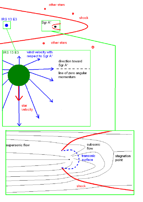
Figure 1: The schematic picture of the wind flow from the star IRS 13E3 towards the Galactic center.

Stellar winds originating from the central cluster are plentiful sources of gas. Most of this material is likely to be expelled from the central region (e.g. Quataert 2004) but a remaining fraction may power the observed activities. Among various mass loosing stars, particularly active one is the Wolf-Rayet star IRS 13 E3 (Paumard et al. 2001, Melia & Falcke 2001), resolved to consist actually of two dusty Wolf-Rayet stars (Maillard et al. 2004). The potential role of each source in dominating the flow pattern can be estimated through its ram pressure (e.g. Melia 1992).

We consider the stars listed by Rockefeller et al. (2004) as potential important sources of the material. For each of the stars independently we calculate the ram pressure, $0.5\rho_{wind}v_{wind}^{2}$ at the location of Sgr A*, where $\rho_{wind}$ is the density of the stellar wind and $v_{wind}$ is the wind velocity. Wind density can be found knowing the outflow rate, $\dot{M}_{wind}$ and the distance, $D_{*}$, from the star to Sgr A*. As a reference, we use IRS 13 E3. Therefore, the ram pressure ratio of a given star to IRS 13 E3 is defined as

$$f_{ram}={\dot{M}_{wind}\over\dot{M}_{o}}{v_{wind}\over v_{o}}({D_{o}\over D_{*}})^{2},$$ (1)

where the quantities $\dot{M}_{o}$, $v_{o}$ and $D_{o}$ are the wind outflow, wind velocity and the distance to Sgr A* of IRS 13 E3. As distance values, $D_{*}$ and $D_{o}$ we use values given by Rockefeller et al. (2004) obtained assuming that the z coordinate of each star is random. Results are given in Table 1.

Source	$f_{ram1}$	$f_{ram2}$
IRS 16NE	0.11	0.027
IRS 16NW	0.01	0.02
IRS 16C	0.05	0.26
IRS 16SW	0.22	0.62
IRS 13E3(AB)	1.0	1.0
IRS 7W	0.054	0.08
IRS 15SW	0.011	0.02
IRS 15NE	0.018	0.02
IRS 29N	0.013	0.07
IRS 33E	0.1	0.02
IRS 34W	0.029	0.027
IRS 16SE	0.014	0.03

Table 1: Results:Values of ram pressure, with the reference source IRS13 E3, for two different values of z coordinate of the source. In the first column the ram pressure was calculated assuming that z coordinate is taken from random distribution, the second column is for z coordinate modeled in Rockefeller et al. (2004).

Source	D	$V_{wind}$	$V_{star}$	$\lambda_{1}[R_{schw}c]$	${\cal E}_{1}/c^{2}$	$\lambda_{2}[R_{schw}c]$	${\cal E}_{2}/c^{2}$	$\dot{M}_{wind}$	$\dot{M}_{1,accr}$	$\dot{M}_{2,accr}$
	[arcsec]	[km/s]	[km/s]					$(10^{-5}M_{\odot}/yr)$	$(10^{-5}M_{\odot}/yr)$	$(10^{-5}M_{\odot}/yr)$
IRS 16NE	3.4	750	560	25.0	$2.0\cdot 10^{-6}$	16.98	$3.99\cdot 10^{-6}$	9.5	1.0	0.66
IRS 16NW	8.36	750	290	3.8	$1.98\cdot 10^{-6}$	2.57	$3.97\cdot 10^{-6}$	5.3	0.09	0.06
IRS 16C	4.6	650	430	19.47	$1.99\cdot 10^{-6}$	12.14	$3.98\cdot 10^{-6}$	10.5	0.94	0.59
IRS 16SW	2.8	650	540	54.13	$2.04\cdot 10^{-6}$	33.7	$4.01\cdot 10^{-6}$	15.5	3.8	2.35
IRS 13E3(AB)	3.8	1000	207	2.16	$1.98\cdot 10^{-6}$	1.68	$3.97\cdot 10^{-6}$	79.1	2.6	1.58
IRS 7W	8.3	1000	380	1.92	$1.98\cdot 10^{-6}$	1.5	$3.97\cdot 10^{-6}$	20.7	0.14	0.1
IRS 15SW	13.4	700	200	1.94	$1.98\cdot 10^{-6}$	1.27	$3.97\cdot 10^{-6}$	16.5	0.13	0.08
IRS 15NE	11.5	750	150	1.34	$1.98\cdot 10^{-6}$	0.91	$3.97\cdot 10^{-6}$	18.0	0.16	0.1
IRS 29N	8.56	750	220	2.71	$1.99\cdot 10^{-6}$	1.84	$3.97\cdot 10^{-6}$	7.3	0.12	0.08
IRS 33E	3.05	750	230	8.0	$1.99\cdot 10^{-6}$	5.43	$3.89\cdot 10^{-6}$	7.3	0.9	0.65
IRS 34W	5.8	750	280	5.26	$1.99\cdot 10^{-6}$	3.56	$3.97\cdot 10^{-6}$	7.3	0.27	0.18
IRS 16SE	8.33	750	540	9.44	$1.99\cdot 10^{-6}$	6.4	$3.98\cdot 10^{-6}$	7.3	0.13	0.08

Table 2: Results:$\lambda_{1}$ and $\dot{M}_{1,accr}$ corresponds to wind temperature $T_{wind}=0.5keV$, $\lambda_{2}$ and $\dot{M}_{2,accr}$ to $T_{wind}=1.0keV$. Mass accretion rate is defined here as $\dot{M}_{accr}=\dot{M}_{wind}\cdot(\frac{R_{BHL}}{D})^{2}$.

Politropic index $\gamma=1.6$.

We see that $f_{ram}$ is smaller than 1 for all stars. The highest value, obtained for IRS 16 SW is equal to 0.22. For another choice of z coordinates of stars (see Rockefeller et al. (2004)), the results are similar. The highest $f_{ram}$=0.62, still smaller than 1, is again for IRS 16 SW.

A number of O type stars not listed in Table 1 also contribute to the mass accretion rate, as discussed by Loeb (2004). However, the closest stars have too high relative velocity with respect to Sgr A* to allow for mass settlement. For example, SO-16 at the closet approach (0.0002 pc) has the velocity of 12 000 km s^-1 and its wind create a narrow stream of gas not directed toward Sgr A*. Stars with velocities of 1000 km s^-1 can lead to an accretion event if they are at the distance of 0.015 pc or more. If we consider a star at such a distance that its Keplerian velocity is equal to the wind velocity we obtain the maximum value of the ram pressure ratio for the star

$$f_{ram}^{max}={\dot{M}_{wind}\over\dot{M}_{o}}({v_{wind}\over v_{o}})^{3}.$$ (2)

If $\dot{M}_{wind}\sim 10^{-6}M_{\odot}$yr^-1 and $v_{wind}\sim 3000$ km s^-1 occasional episodes of strong accretion from such a star are expected, in agreement with Loeb (2004) estimates but if $\dot{M}_{wind}\sim 10^{-6}M_{\odot}$yr^-1 and $v_{wind}\sim 3000$ km s^-1 then $f_{ram}\sim 0.08$ and the wind will be confined by the wind from IRS 13 E3.

In further considerations we assume that the wind of IRS 13 E3 dominates at the position of Sgr A*, i.e. it is strong enough to form a bow shock which shields Sgr A* from the winds from other stars. In order to check whether this assumption is not in contradiction with the observations we check the predicted wind density. The adopted wind outflow rate, wind velocity and the distance (see Table reftab:stars) the wind density at the location of Sgr A* (neglecting at this moment the gravitational effect of the black hole) is 108 cm^-3. This value is consistent with the density 130 cm^-3 measured by Baganoff et al. (2003) within the radius 1.4” of Sgr A*.

2.2 Angular momentum of the flow

We assume now that IRS 13 E3 is the dominant source of the matter accreting onto Sgr A^∗. We determine the net angular momentum of the flow in the following way:

We consider the case where the wind velocity is much higher than the orbital velocity of a star. Therefore, the material ejected from a fractional region of the star surface located at $\phi_{o}$ (see Fig.1) can reach the gravity center with zero angular momentum (see e.g. Loeb 2004). This angle is given by the condition:

$$\sin\phi_{o}={v_{star}\over v_{wind}}.$$ (3)

The wind is mildly supersonic, with the Bondi-Hoyle-Lyttleton accretion radius, $R_{BHL}$, given by the formula

$$R_{BHL}={2GM\over v_{wind}^{2}+v_{s}^{2}},$$ (4)

where $v_{wind}$ is the flow velocity and $v_{s}$ is the sound speed within the wind.

The spherically-symmetric wind blowing at $\phi\neq\phi_{o}$ or out of the orbital plane will posses some amount of positive or negative specific angular momentum (angular momentum density), $l$. In the second order approximation

$$l\approx-v_{wind}D\delta\phi\cos(\phi_{o})[1-1/2\tan\phi_{o}\delta\phi],$$ (5)

where $\delta\phi=\phi-\phi_{o}$, $\phi$ is the azimuthal angle of the element at the star surface and $D$ is the distance between the star and the Galactic center.

A cylindrical fraction of this flow, with $\Delta\phi=R_{BHL}/D$, and $\Delta\theta\sim R_{BHL}/D$ will be intercepted by the central black hole, where the angle $\theta$ determines the deviation from the orbital plane. Integrating the Equation 5 with respect to $\delta\phi$ and $\delta\theta$ in the limits specified by $\Delta\phi$ and $\Delta\theta$, we obtain the net angular momentum of the flow as:

$$l_{eff}={2\over 3\pi}{1\over\sqrt{1-(v_{star}/v_{wind})^{2}}}v_{star}D\left({R_{BHL}\over D}\right)^{2},$$ (6)

The above relation is valid if the star velocity is significantly smaller than the wind velocity. Large value of the angular momentum density of the donor star, $v_{star}D$, is decreased by small quadratic term in the $R_{BHL}/D$ ratio.

We further express the angular momentum density in dimensionless units $2GM/c$, or equivalently

$$\lambda={l_{eff}\over R_{Schw}c},$$ (7)

where $R_{Schw}=2GM/c^{2}$.

We calculate the values of $\lambda$ for each of the stars in Table 1. We consider two values of the temperature representative for the possible wind temperature: 0.5 keV and 1.0 keV (eg. Muno et al.2004, Raassen et al. 2003). We calculate angular momentum $\lambda$ for these two values of wind temperature , $\lambda_{1}$ (also Bernoulii constant ${\cal E}_{1}$) corresponds to 0.5 keV , $\lambda_{2}$ (and ${\cal E}_{2}$) to 1.0 keV.

In the case of the temperature of 0.5 keV the average value of $\lambda$ calculated for all stars is 12.2, and if we neglect the dominant star IRS 13 E3 this mean value is equal to 13.3. It is interesting to compare this value with the mean angular momentum obtained in hydrodynamical simulations in the innermost part of the flow. In dimensionless units, these values are $\sim 25$ in Cuadra et al.(2005b), $\sim 40-60$ in Coker $\&$ Melia (1998), and 3-20 in Coker $\&$ Melia (1997), not far from our results. However, as we showed above (see Sect. 2) actually the star IRS 13 E3 dominates the flow and the effective angular momentum is ten times lower. It shows that using equally efficient stellar winds in the simulations may lead to unrealistic description of the flow.

2.3 Flow geometry within $R_{BHL}$ and the Bernoulli constant

The supersonic flow develops a shock at a distance to the black hole comparable to $R_{BHL}$, as shown in a number of papers addressing the issue of the supersonic motion of the accreting objects (e.g. Salpeter 1964, Bisnovatyi-Kogan 1979). The topology of solutions was systematically discussed by number authors (Hunt 1971, 1979, Livio et al. 1979, Okuda 1983, Livio et al. 1986, Shima et al.1986, Matsuda 1992, Ishii et al. 1993 Ruffert 1994,1995,1996) Three dimensional calculations recently were made by Pogorelov et al. (2000), and Foglizzo et al. (2005).

Since black hole has no rigid surface the shock does not initially form in front of it but only sideways, as sketched in Fig. 1. Shocked material returns toward the black hole and the dominant inflow actually comes from this back-side flow. Since the infalling material has certain small angular momentum and the density slowly decreasing perpendicularly to the flow in the same direction as the donor star velocity the flow patters is not symmetric with respect to the main axis. The stagnation point is shifted, and the material with the lowest and the highest angular momentum mix.

We can determine the Bernoulli constant of this material, $\cal E$, either above or below the shock. Its value above the shock can be estimated as

$${\cal E}={1\over 2}v_{wind}^{2}+{v_{s,wind}^{2}\over\gamma_{i}-1}-{GM\over(R_{BHL}-R_{Schw})}+{1\over 2}{\lambda^{2}\over R_{BHL}^{2}}$$ (8)

assuming that the velocity of the wind close to the shock is equal to initial wind velocity, and that the shock occurs at distance comparable to $R_{BHL}$. In Eq. 8 the second term dominates, so the Bernoulli constant is mainly determined by assumed wind temperature $T_{wind}$ and politropic index $\gamma$.

Values of $\cal E$, in $c^{2}$ units, are given in Table 1, for two values of the wind temperature. Because for a supersonic wind the Bernoulli constant $\cal E$ is $\sim v_{s,wind}^{2}/v_{wind}^{2}\times\frac{3-\gamma}{2(\gamma-1)}$ all values of $\cal E$ in the Table 2 are almost the same for corresponding temperature of the wind.

For IRS 13 E3 they are of order of $(1-4)\times 10^{-6}$. In calculations we adopt $\lambda$=2.16 and $\cal E$ for $T=0.5$ keV before the shock as appropriate for consideration of the accretion close to Sgr A*. Because we assume adiabatic shocks, the Bernoulli constant doesn’t change after passing the shock. Keeping the Bernoulli constant we obtain temperature of the gas after a shock to be $T=1.4keV$ (for parameters adopted for Sgr A*). This value seems to be in a good agreement with X-ray observations of Sgr A* (Baganoff et al. 2003).

In order to simplify the issue we further assume that the accretion proceeds roughly in a spherically symmetric way, with the effective angular momentum given by Eq. 6 and the Bernoulli constant determined from Eq. 8. This simplification allows to use the semi-analytical solution for the flow pattern outlined in the next section.

3 Low angular momentum flow close to Sgr A*

Therefore, we further study the low angular momentum (strongly sub-Keplerian) flow onto Sgr A^∗. Apart from Cuadra et al. (2005a,b), only a few papers were devoted to this option so far. Melia (1994) considered a model of a free fall with non-negligible angular momentum assuming no contribution to emission from within the circularization radius. Proga & Begelman (2003a,b) performed 2-D hydrodynamical and magnetohydrodynamical simulations of the low angular momentum flow for a specific class of outer boundary conditions (angular momentum decreasing with the distance from the equatorial plane).

Here we concentrate on semi-analytical solutions with standing shocks in the pseudo-Newtonian potential.

3.1 General character of the low angular momentum flow

The initially subsonic flow onto a black hole must exhibit transonic behavior in order to satisfy the inner boundary conditions imposed by the event horizon, i.e. it becomes supersonic again.

Low angular momentum flow may actually posses more than one sonic, as first shown by Abramowicz & Żurek (1981). Typically the external sonic point, $r_{out}$, lies far from the black hole (close to a Bondi radius for a corresponding spherical accretion). The internal sonic point, $r_{in}$, and the middle sonic point $r_{mid}$ exist within and outside the marginally stable orbit, respectively, for general relativistic (Das 2004, Barai, Das & Wiita 2004) as well as for post-Newtonian (D02, DPM) model of accretion flow. The location of the sonic points can be calculated as a function of the specific flow energy ${\cal E}$ (the Bernoulli’s constant), angular momentum $\lambda$ and inflow polytropic index $\gamma_{i}$ (see, e.g. §3 of D02 for details of such calculations).

If $\lambda$ is close to zero, a shock does not form, and accretion remains supersonic down to the event horizon after it crosses $r_{out}$. For slightly larger $\lambda$ the centrifugal barrier becomes strong enough, inflowing matter starts pilling up close to the black hole due to the resistance offered by the barrier, and the depleted matter may break the incoming flow behind it and consequently a shock forms. Such shocks may become steady and standing so that they can be studied within the framework of stationary flow (D02, DPM and references therein).

Following D02, we consider here a stationary non self-gravitating, non-magnetized, inviscid accretion of polytropic fluid. We assume that the flow proceeds through a standing shock, so the discontinuity in the radial velocity allows to match the supersonic flow below $r_{out}$ with the transonic flow through $r_{in}$. The exact location of the shock as a function of parameters $\left[{\cal E},\lambda,\gamma_{i}\right]$ is obtained by solving the generalized Rankine-Hugoniot equations. We assume that the shock is non-radiating and infinitesimally thin.

However, for the parameters chosen as the best values for the accretion flow onto Sgr A* (${\cal E}=2\times 10^{-6}-4\times 10^{-6}$ , $\lambda=1.68-2.16$ and $\gamma_{i}=1.6$, see results for IRS13E3 in Table 1) we do not obtain a stationary solution describing the accretion all the way down to the black hole.

In order to understand what is happening we analyze the model properties in the broader parameter space around the adopted values.

3.2 Dependence of the flow topology on model parameters

For a fixed $\gamma_{i}$ and ${\cal E}$ the position of the sonic point and the position of the shock are strong functions of $\lambda$. The equation of motion with small angular momentum allow us to determine the position of the sonic points:

$${\rm{v^{2}}\over 2}+{\rm{v_{s}^{2}}\over\gamma-1}-{GM\over r-R_{g}}+{\lambda^{2}\over 2r^{2}}=\cal E$$ (9)

Derivative of Eq.9 can be expressed as:

$$\rm{v{dv\over dr}}=\frac{{2\over r}\rm{v^{2}}-{GM\over(r-R_{g})^{2}}+{\lambda^{2}\over r^{3}}}{1-{v^{2}\over v_{s}^{2}}},$$ (10)

with the help of the continuity equation. The sonic point condition is that nominator and denominator of Eq.10 equals zero. In the upper panel of Fig. 2 we show the position of sonic points, as functions of $\lambda$ parameter for constant Bernoulli constant ${\cal E}=1.98\times 10^{-6}$ in $c^{2}$ units.

For $\lambda$ lower than about 1.4 (in general for any Bernoulli constant), one solution of equations Eq.9 and Eq.10 exist above the black hole horizon for introduced gravitational potential. This point is located at a large distance from the black hole and the flow proceeds as in the case of a spherical Bondi flow. For $\lambda$ between $\sim 1.4$ and $\sim 20$ (in general upper value of $\lambda$ is a function of specific flow energy $\cal E$) three formal solutions exist. However, there is a significant difference between the solutions for $\lambda$ smaller than 2 and larger than 2. For $\lambda$ smaller than $\sim 2.0$ (exact limit slightly depends on $\cal E$) the inner sonic point describes the physically acceptable solution for the inflow. However, for $\lambda$ larger than $\sim 2.0$ the internal sonic point is unphysical, in this point $v_{s}^{2}$ is less than zero (see Abramowicz & Żurek 1981 for the discussion). The transition from physical to unphysical inner sonic points takes place for $\lambda$ very close to 2 (the dependence on $\cal E$ is of order of $\cal E$ in our dimensionless units. In Fig. 2 (upper panel) we mark the unphysical points with dashed line, and the physical points with solid line.

For $\lambda$ still larger than $\sim 20$ again one sonic point exists (unphysical ones), it is located under the last stable orbit (sonic point position approach to 1 $R_{g}$) and the flow proceeds in a subsonic way. This type of solution finally becomes unphysical since in the case of higher angular momentum subsonic flow it is unlikely that the angular momentum transfer is negligible and the appropriate solution of the physical flow is provided by ADAF-type models.

In the lower panel of Fig. 2 we expand the figure around most plausible values of $\lambda$ for Sgr A*, and we mark the position of the stationary shock with the dashed line. We see that this type of solutions exist in a very narrow range of the physical parameters, as noted before in D02.

Fig. 2 was obtained for a specific value of the Bernoulli constant but the dependence on it is not very strong. In Fig. 3 we show the positions of the sonic points as functions of $\cal E$ for fixed $\lambda$, for higher initial wind temperature 1.0 keV. Stationary shock develops only for the Bernoulli constant a few times lower that the value estimated for Sgr A*. The same picture is not possible for $\lambda=2.16$ because in the case of $\lambda>2$ the inner sonic points are unphysical, so the transonic accretion for lower specific energy of the flow is still not possible. Changing of $\cal E$ is changing only the position of the outer sonic point (as shown in Fig. 3), so in a case of $\lambda>2$ with lower $\cal E$ the topology will not change.

We can mark conveniently the types of solutions using the $\cal E$ - $\lambda$ diagram (see Fig. 4), as introduced in D02. We have four regions in the interesting range of parameters for Sgr A*. Region A corresponds to semi-spherical flow without a shock and when we have only one distant sonic point. In region B three sonic points exist, the condition for a stationary shock is never satisfied but the flow proceeds supersonically without a shock.

Fig. 5 shows the topology of the shocked accretion flow for the values of the Bernoulli constant $\cal E$ and $\gamma_{i}$ appropriate for Sgr A*, but with angular momentum $\lambda=1.55$, lower than the best estimate for Sgr A*. Such a topology is representative for region C. For such $\lambda$ the stationary shock is possible. Matter first passes through $r_{out}$ ( $\sim 10^{4}$ $r_{g}$) and encounters a shock at $r_{sh}$ ($\sim$ 70 $r_{g}$) close to the black hole. The solid vertical line marked with a down-ward arrow represents the shock transition. $M_{-}$ and $M_{+}$ are the pre/post shock Mach numbers and the shock strength ${\cal S}$ is defined as ${\cal S}=\frac{M_{-}}{M_{+}}$, which comes out to be 4.0 for this case. Post-shock subsonic inflow becomes supersonic again after crossing $r_{in}$ ( 3.1 $r_{g}$) and finally dives through the event horizon.

Figure 2: The position of the sonic points as functions of the angular momentum for the Bernoulli constant appropriate for Sgr A* accretion flow. Lower panel shows the expanded version of the upper graph, with the position of the shock marked with the dashed line. For $\lambda=2.16$ no stationary shock solution exists.

Figure 3: The position of the sonic points as functions of the Bernoulli constant for angular momentum $\lambda=1.68$ appropriate for Sgr A* accretion flow. Position of the shock is marked with the dashed line.

Figure 4: Region A corresponds to semi-spherical flow without a shock and with a distant sonic point and inner under horizon, in region B four sonic points exist, the condition for a stationary shock is never satisfied but the flow proceeds transonically without a shock. In region C a stationary shock solution exists, D region corresponds to the parameters for which torus form. Plausible parameters of the inflow in Sgr A* locate the solutions in region D (thick continuous line).

Sgr A*, however, lies in the region D, according to our estimates. In the region D, three sonic points still exist but the topology is different, the initially supersonic flow proceeds along the flow line which end up at a distance of few Schwarzschild radii, since the flow line forms there a closed loop (see Fig. 6). The angular momentum barrier is just strong enough to prevent the flow

This dependence of the topology on the flow parameters was discussed before (see D02, Das 2004, Chakrabarti & Das 2004). However, most of the attention in those papers was payed to models with stationary shocks, located in region C. What is new and important is that our best estimates of the flow in Sgr A* locate the flow in the D region, where no stationary shock develops.

Figure 5: The topology of the flow obtained wit a standard stationary shock solution for angular momentum lower than that for Sgr A*. Dotted line marks the position of the line where Rankine-Hugoniot conditions are satisfied, so the intersection of this line with the transonic flow lines marks the position of the shock (arrows). Inner shock is unstable, outer shock is stable. Sonic points are marked with pluses ’+’.

Figure 6: The topology of the flow obtained for the flow parameters corresponding to Sgr A*. Close loop touches the radius of 4 $R_{Schw}$ in a case of $\lambda=1.68$ or 10 $R_{Schw}$ in a case of $\lambda=2.16$ and the constant angular momentum torus forms there.Sonic points marked with pluses ’+’.

This means that the flow in Sgr A* is non-stationary in a natural way, and it consists of two parts:

• outer, semi-stationary flow

• inner, non-stationary torus

3.3 Constraints on mass accretion rate from Faraday rotation in an outer flow

Our model gives self-consistent constraints on the mass accretion rate, which is estimated from the conditions at the position of the first outer sonic point. The values of mass accretion rate estimated by this condition are given in Table 3. In Table 2 we showed the accretion rate calculated using the formula: $\dot{M}_{accr}=\dot{M}_{wind}\cdot(\frac{R_{BHL}}{D})^{2}$, which is about an order of magnitude larger than the one calculated at the position of the sonic point. Thus we assume here that there must be an outflow at some radius, but we do not specify its form or geometry.

$\lambda$	$\dot{M}_{sonicpoint}[M_{\odot}/yr]$	$RM[rad/m^{2}]$
0.82	$3.93\cdot 10^{-6}$	$5.7\cdot 10^{5}$
1.68	$2.45\cdot 10^{-6}$	$7\cdot 10^{5}$
2.16	$2.18\cdot 10^{-6}$	$2\cdot 10^{6}$
12.2	$2.15\cdot 10^{-6}$	$2.8\cdot 10^{6}$

Table 3: Mass accretion rate for four values of angular momentum $\lambda$ parameter.

We compare our results with the limitations estimated from Faraday rotation measurements, which give us a limit for the mass accretion rate very close to the black hole (up to 100 $R_{SCHW}$). In general such high accretion rates as shown in Table 3 give RM coefficient to be very high in comparison to the data. For non relativistic plasma the rotation measured is given by:

$$RM=8.1\cdot 10^{5}\int n_{e}\vec{B}d\vec{l}$$ (11)

For ultra-relativistic thermal plasma ($Te>6.0\cdot 10^{9}$) RM have to be additionally multiplied by a factor of $\frac{log\gamma}{2\gamma^{2}}$ (Quataert $\&$ Gruzinov 2000). Taking into account our $n_{e}(r)$ profile and the absolute value of the magnetic filed (which is in equipartition with the gas) we obtain RM to be overestimated. However, the magnetic field of the inflowing material is unlikely to have large scale structure. Indeed, from magnetohydrodynamical simulations of accretion of plasma with low angular momentum we know that if we include changing of the direction of the magnetic field along any specific line of sight the RM factor is reduced even a few hundred times (Moscibrodzka et al. 2006, in preparation). Assuming the reduction factor of 200 the results, given in Table 3, are consistent with the recent measurements of RM for Galactic center where RM is from few times $10^{5}rad/m^{2}$ to few times $10^{6}rad/m^{2}.$ (Bower et al. 2005, Quataert $\&$ Gruzinov 2000).

3.4 Stationary emission from the outer part of inner flow

The outer part of the inner flow, from the Bondi radius down to the inner radius of the closed loop in Fig. 6 can be considered approximately as a stationary. Knowing the flow parameters, we can calculate the radiation spectrum of such a flow, and we expect it to represent the stationary, non-variable emission of Sgr A*.

We use the model outlined in Mościbrodzka et al. (2005). This model is based on the assumption that the flow is two-temperature, with the flow dynamics mostly determined by ions. Electrons are heated partially due to the Coulomb coupling with ions, but also $\delta$ fraction of energy goes directly to electrons through the Ohmic heating. The presence of the magnetic field is assumed, with the field strength measured with respect to the equipartition value through the $\beta$ parameter. The emission is calculated with the use of the Monte Carlo code, taking into account bremsstrahlung, synchrotron emission and Comptonization.

Figure 7: The stationary emission of the Sgr A* flow generated between the outer radius, which is about 2 Bondi radii and the inner radius determined by the distance of the closed loop flow from the black hole. For $\lambda=1.68$ the inner loop close at distance 4.0 $R_{Schw}$ , for $\lambda=2.16$ the loop close at about 10 $R_{Schw}$ and spectrum is marked as long dashed and solid line respectively. The spectrum marked as dotted line is calculated for the mean value of specific angular momentum $<\lambda>=12.2$ of all available sources of matter, in this case the torus forms at about 1000 $R_{g}$. For $\lambda=0.82$ (the case of IRS 13 but with the assumption that the star cluster is located 10 arcsec from the center), the flow is continuous down to the event horizon without formation of a shock and the spectrum is marked as short dashed line.

Models in Mościbrodzka et al. (2005) were based on spherical accretion dynamics but now we generalized to the case of the flow with low angular momentum, described in Section 3.2. The adopted parameters for modeling emissivity are $\beta=0.5$ and $\delta=0.5$.

The spectra calculated for four representative values of the angular momentum are shown in Fig. 7.

The most satisfactory representation of the broad band stationary emission is provided by the model with $\lambda=2.16$. It fits the quiescence NIR spectrum quite well and does not overpredict the stationary X-ray emission measured by Chandra. The spectral slope of the modeled X-ray emission is within the error bars of the data. The radio tail is not reconstructed. To fit radio part of the spectrum, we need a non-thermal population of electrons (Yuan et al. 2003), currently not included in the model. The model with $\lambda=1.68$ is slightly too bright in the X-rays and in the IR. This is due to the fact that the inner boundary of a stationary flow is further out for $\lambda=2.16$ and closer in for $\lambda=1.68$.

Since our determination of the most plausible range of angular momentum is the accreting flow is based on a number of assumptions, we also show the resulting spectrum for a lower, and a higher value of $\lambda$.

The solution $\lambda=0.82$ corresponds to a distance of IRS13 of 10 arcsec. Such a solution has different topology, as seen from Fig. 4. It belongs to the region A, which means that a single (outer) sonic point exists, and the flow is practically as in the case of a flow without angular momentum. Flow velocity is high and the density is relatively low although the accretion rate required by the condition of transonic solution is actually slightly higher than in the two cases considered before. Therefore, the radiative efficiency of the flow becomes lower although the stationary flow proceeds down to the black hole horizon. The resulting spectrum (see Fig. 7) underrepresent the X-ray persistent emission by more than an order of magnitude.

The solution $\lambda=12.2$ corresponds to the assumption that the ram pressure cannot prevent accretion streams from various stars to approach Sgr A* (i.e. the value of the angular momentum is given as a mean value for all stars from Table 2). This solution belongs to region D in Fig. 4. The high value of the angular momentum prevents the stationary flow from approaching a black hole - the accumulation radius is $\sim 1000R_{Schw}$. The level of emission is very low and the spectrum and none of the observational points are reproduced. It may not conclusively rule out all higher angular momentum models since the model of constant angular momentum flow is not likely to apply to the flow with high initial angular momentum. Effects of the angular momentum transfer may in such case take place, as suggested by the numerical simulations (e.g. Cuadra et al.2005). The issue can be set by future MHD simulations with appropriate grid coverage, realistic boundary conditions and computations of the resulting spectra.

3.5 Inner torus

At the inner radius of the semi-stationary flow, the inflowing matter accumulates and forms a ring of material with constant angular momentum. The exact location of the torus/ring depends on the angular momentum. For $\lambda=1.68$ it forms very close to the marginally stable orbit. For $\lambda=2.16$ (determination for IRS 13 E3 assuming lower wind temperature; see Table 1) the topology of the solution is again as in Fig. 6 but the ring forms at 10 $R_{Schw}$.

The equilibrium of the material with fixed angular momentum close to a black hole has been studied long time ago (Abramowicz, Jaroszyński & Sikora 1978, Jaroszyński, Abramowicz & Paczyński 1980). The key parameter here is the exact value of $\lambda$. If $\lambda<2$ then the equipotential surface exists with an inner cusp. As soon as the material fills this equipotential surface the accretion proceeds. This means that the inflow is completely rebuilt and the initial mostly supersonic inflow is replaced with the solution which is subsonic above the marginally stable orbit. It is represented by the lower line in Fig. 6. Such a solution, if reached, would remain stable. However, the timescale to built this flow pattern is long. For our $\lambda=1.68$ solution the mass in the supersonic branch (upper transonic solution in Fig. 6) is $M_{1}=1.28\times 10^{-5}M_{\odot}$, the mass in the subsonic branch (the lowest branch in Fig. 6 in lower panel) is $M_{2}=1.22\times 10^{-5}M_{\odot}$, and the accretion rate on the transonic branch is $\dot{M}=2.45\times 10^{-6}M_{\odot}yr^{-1}$, so the reconstruction timescale is roughly $(M_{2}-M_{1})/\dot{M}=0.26$ yr.

On the other hand, the newly formed ring is known to be strongly unstable, roughly in the local dynamical timescale (Papaloizou & Pringle 1984). Actually, a ring model as an explanation of the Sgr A* variability (e.g. Liu & Melia 2002, Rockefeller et al 2005, Prescher 2005, Tagger & Melia 2006). Therefore, we find it extremely interesting that the best estimates of the accretion flow parameters leads in a natural way to formation of such a ring.

Calculation of the dynamics and the spectra of this ring is beyond the scope of the present paper. We can only speculate, that the matter in a ring accumulates as long as the density contrast between the ring and the infalling material is large enough. In that case the (non-stationary) shock forming between the ring and the inflowing material can effectively reflect the instability waves and the torus is violently disrupted. Most of the material plunges into black hole or is ejected in a form of a jet. However, small fraction of the material may remain in a ring-like configuration, with increased angular momentum. Hydrodynamical simulations (Żurek & Benz 1986, Hawley 1987; see also Proga & Begelman 2003ab and the references therein) and analytic studies in the non-linear regime (Goodman, Narayan & Goldreich 1987) support the instability scenario but the long time-scale behavior of the flow under such conditions is not determined yet. The magnetic field is also likely to play a role in redistribution of the angular momentum (e.g. De Villiers & Hawley 2003, Tagger & Melia 2005) or producing an outflow.

4 Discussion

The accretion flow into Sgr A* black hole is widely believed to be radiatively inefficient but the exact character of the inflow is under discussion. In the present paper we estimated analytically the effective angular momentum of the accretion flow by analyzing the relative strength of the winds of the nearby stars.

We calculated ram pressure from each of the sources listed in Table 2. Assuming the stellar wind properties, positions and velocities given in Rockefeller et al. (2004) we argue that IRS 13E3 dominates. This star complex would stop dominate if it was more than 5 arcsec far away from the center. If IRS 13 is further away IRS16 SW would be a dominating source instead, because it has second high mass accretion rate. In such case the angular momentum supplied by this star complex would be too high to accrete directly closer than $10^{6}R_{SCHW}$. An angular momentum transfer would be requested to power Sgr A* and the dynamics would be like in ADAF flow. On the other hand if we slow down the wind of IRS 13 has a velocity of 650 km/s (the same value as of IRS 16SW), with the distance unchanged, then IRS13 still dominates.

Therefore, we favor the scenario in which the wind from the IRS 13 E3 complex dominates, and the angular momentum, $\lambda$, is of order of 1.68 - 2.16 in dimensionless units ($R_{Schw}c$). (Angular momentum provided by IRS 13E3 can change due to ellipticity of the orbit ,and the picture of accretion flow can change. The issue concerning ellipticity of orbits was discussed in context of very near stars with short periods (Loeb 2004), but it is not discussed in this paper.) . This value is much lower than usually adopted in the outer part of the ADAF-type flow. Thus we analyzed the flow in the pseudo-Newtonian potential following the original ideas of Abramowicz & Żurek (1981) (see Das 2004 for recent developments) allowing for a multi-transonic solution for constant angular momentum. We found that the angular momentum estimated for Sgr A* is just large enough to provide the centrifugal barrier close to the black hole. Therefore, the inflow is mostly supersonic but close to the black hole the stationary solution does not exist and the material piles up. The radius, where an inner ring/torus forms depends significantly on the exact value of the angular momentum, and for $\lambda$ between 1.68 - 2.16 it falls into 4 - 10 $R_{Schw}$ range. We assumed that the inflow region is the source of the persistent emission and we calculated the radiation spectrum for the two extreme cases of $\lambda$ equal to 1.68 and 2.16, taking into account bremsstrahlung, synchrotron emission and Comptonization. The accretion rate ($\dot{M}=4.29\times 10^{-6}M_{\odot}yr^{-1}$) was determined self-consistently from the model, from the condition of the transonic inflow in the outer region. Taken at the face value, this accretion rate overpredicts the observed Faraday Rotation measure by two orders of magnitude (Bower 2003,2005). However, we find that if magnetic field is very tangled, then this accretion rate does not violate this limits.

The case of larger $\lambda$ gave the spectrum roughly consistent with the persistent emission, the case of smaller $\lambda$ overpredicted the persistent emission level.

The inner ring/torus was not modeled in our paper, but is is well known that such a constant angular momentum ring is a subject to violent instabilities (Papaloizou & Pringle 1984) which opens an attractive scenario for modeling SGR A* flares. Therefore, our estimates of the inflowing material parameters support the models based on the presence of an inner torus (e.g. Liu & Melia 2002, Rockefeller et al. 2005, Prescher 2005, Tagger & Melia 2006).

Our analytical estimates are necessarily oversimplified, and it would be interesting to see whether 3-D computations, like those of Cuadra et al. (2005a,b) give the same result if the dominant role of IRS 13E3 is taken into account. However, this is not simple since it requires modeling also in the supersonic region.

If our estimates of the angular momentum and the accretion rate are correct then we deal with two issues important for the long timescale studies.

First issue concerns the accretion rate secular changes. In our model the wind accretion rate given in Table 1 is by a factor of 3 - 5 higher than the accretion rate through the outer sonic point. This means that some material is temporarily stacked there, at distance of a few thousands $R_{Schw}$. We estimated the timescale for the radiative cooling in this region from our model and this timescale is long ($2.8\times 10^{6}$ yr) which means that the material remains hot. Second issue is the cumulating angular momentum of the material in the innermost part of the flow. The inner ring/torus instabilities cause events of accretion but a fraction of the material has to remain to carry the excess angular momentum and a kind of equatorial outflow/drift of high angular momentum material is likely to develop. Therefore, we can expect some kind of instability in a longer timescale, when this accumulating material finally forms a type of an ADAF inflow with much higher accretion rate. Such periods of enhanced accretion probably occasionally happen in Sgr A* (for evidences for an enhanced luminosity about 300 yr ago, see Revnivtsev et al. 2004). Unfortunately, performed numerical simulations do not cover yet timescales and radial ranges wide enough to see such phenomenon.

5 Conclusions

Our analysis of the flow pattern in Sgr A* indicates that

• If IRS13 distance to Sgr A* in 3D is close to its projected distance of about 3.5, IRS 13E3 is a single dominant source of the material for Sgr A* activity, and the number density of its wind estimated near Sgr A* is roughly consistent with the X-ray data limits of Baganoff et al. (2003)

• the estimated mean angular momentum density $\lambda$ of the inflowing is most likely between 1.68 and 2.16 in $R_{Schw}c$ units

• for such an angular momentum and realistic values of the Bernoulli constant no stationary shock solutions exist and the material piles up close to the black hole, forming a (non-stationary) ring/torus

• for $\lambda=2.16$ the inflow stops at $\sim 10R_{Schw}$ and the radiation spectrum (including bremsstrahlung, synchrotron and Comptonized radiation) emitted by the material above this radius is roughly consistent with the persistent emission from Sgr A* (Except of the radio part of the spectrum.)

• for $\lambda=1.68$ inflow stops at $\sim 4R_{Schw}$, and the predicted persistent emission is too high for Sgr A*.

• the accretion rate predicted by our model is consistent with the limits given by the measurements of the Faraday rotation if magnetic field is highly tangled and makes many reversals, reducing the Faraday Rotation measure by 200 times.

References

- [] Abramowicz M.A., Jaroszynski M., Sikora M., 1978, A&A, 63, 221
- [] Abramowicz M.A., Żurek W.H., 1981, ApJ, 246, 314
- [] Abramowicz M.A., Chen X.,Kato S., Lasota J.-P., Regev O., 1995, ApJ, 483, L37
- [] Baganoff F.K. et al., 2003, ApJ, 591, 891
- [] Baganoff F.K. et al., 2001, Nature, 413, 45
- [] Baganoff F.K., 2003, HEAD, 35.0302
- [] Barai, P., Das, T. K., & Wiita, P. J. 2004. ApJ, 613, L49
- [] Belanger G. et al. 2005, ApJ, 635, 1095
- [] Bisnovatyi-Kogan G.S., Kazhdan Y.M., Klypin A.A., et al., 1979, Soviet Astronomy, 23, 201
- [] Beloborodov A.M., Illarionov A.F., 1991, MNRAS, 323, 167
- [] Bisikalo A.A., Boyarchuk V.M., Chechetkin V.M., Kuznetsov O.A., Molteni D., 1998, MNRAS, 300, 39
- [] Bondi H., 1952, MNRAS, 112, 195
- [] Bower G.C., Falcke H., Wright M.C., Backer D.C., 2003, ApJ, 588, 331
- [] Bower G.C., Falcke H., Wright M.C., Backer D.C., 2005, ApJ, 618, 29
- [] Chakrabarti, S. K., Tapas S., 2004, MNRAS, 349, 649
- [] Coker R.F., Melia F., 1997, ApJ, 488, L149
- [] Coker R.F., Melia F., 1998, IAUS, 184, 319
- [] Cuadra J., Nayakshin S., Springel V., Di Matteo T., 2005a, MNRAS, 360, L55
- [] Cuadra J., Nayakshin S., Springel V., Di Matteo T., 2005b, astro-ph/0505382
- [] Das, T. K. 2002, ApJ, 577, 880 (D02)
- [] Das, T. K. 2003, ApJ, 588, L89
- [] Das, T. K. 2004, MNRAS, 375, 384
- [] Das, T. K., & Chakrabarti, S. K. 1999, Class. Quantum Grav. 16, 3879 (DC)
- [] Das, T. K., Pendharkar, J. K., & Mitra, S. 2003, ApJ, 592, 1078 (DPM)
- [] Das, T. K., Rao, A. R., & Vadawale, S. R. 2003, MNRAS, 343, 443 (DRV)
- [] De Villiers J.-P., Hawley J.F., 2003, ApJ, 592, 1060
- [] Eckart A., Genzel R., 1997, MNRAS, 284, 576
- [] Eckart A. et al., 2004, A&A, 427, 1
- [] Eckart A. et al. 2005, astro-ph/0512440
- [] Foglizzo T., Galletti P, Ruffert M., 2005, A&A, 435, 397
- [] Genzel et al., 2003, Nature, 425, 934
- [] Ghez A. et al. 2004, ApJ, 601, L159
- [] Goldwurm et al. 2003, ApJ, 584, 751
- [] Goodman J., Narayan R., Goldreich P., 1987, MNRAS, 225, 695
- [] Hawley J.F., 1987, MNRAS, 225, 677
- [] Ho L.C. 1999, in Observational Evidence For Black Holes in the Universe, ed. S.K. Chakrabarti (Dodrecht: Kluwer), 157
- [] Hunt R., 1971, MNRAS, 154 ,141
- [] Hunt R., 1979, MNRAS, 188 ,83
- [] Igumenshchev I.V., Beloborodov A.M., 1997, MNRAS, 284, 767
- [] Igumenshchev I.V., Abramowicz M.A., 1999, MNRAS, 303, 309
- [] Illarionov A.F., 1988, Sov. Astron., 31, 618
- [] Ishii T., Matsuda T., Shima E., Livio M., et al., 1993, ApJ, 404, 706
- [] Jaroszynski M., Abramowicz M.A., Paczynski B., 1980, AcA, 30, 1
- [] Liang E.P.T., Nolan P.L., 1984, Space Sci. Rev., 38, 353
- [] Liu S., Melia F., 2002, ApJ, 566, L77
- [] Liu S., Perosian V., Melia F., 2004, ApJ, 611, L101
- [] Liu S., Melia F., Perosian V., 2005, astro-ph/0506151
- [] Livio M., Shara M.M., Shariv G., 1979, ApJ, 233, 704
- [] Livio M., Soker N., de Kool M., Savonije G.J., 1986, MNRAS, 222, 235
- [] Loeb A., 2004, MNRAS, 350, 725
- [] Mailard J.P., Paumard T., Slolovy S.R., Rigaut F., 2004, A&A, 423, 155
- [] Maraschi L., Tavecchio F., 2003, ApJ, 593, 667
- [] Markoff S., Falcke H., Youan F., Biermann P.L., 2001, A&A, 379, L13
- [] Melia F., Falcke H., 2001, ARA&A, 39, 309
- [] Miyoshi, M., Imai, H., Nakashima, J., Deguchi, S., Shen, Z., 2005, in Future Directions in High Resolution Astronomy: The 10th Anniversary of the VLBA, ASP Conference Proceedings, Vol. 340. Edited by J. Romney and M. Reid. San Francisco: Astronomical Society of the Pacific, 2005., p.258
- [] Mościbrodzka M., 2005, astro-ph/0512527
- [] Matsuda T., et al., 1992, MNRAS, 255, 183
- [] Narayan R. Yi I., Mahadevan R., 1995, Nature, 374, 623
- [] Okuda T., Teresi V., Toscano E., Molteni D., 2004, PASJ, 56, 547
- [] Okuda T., 1983, PASJ, 35, 235
- [] Paczyński B., Wiita P.J., 1980, A&A, 88, 23
- [] Papaloizou J.C.B., Pringle J.E., 1984, MNRAS, 208, 721
- [] Paumard T., Maillard J.P., Morris M., Rigaut F., 2001, A&A, 366, 466
- [] Pogorelov N.V., Ohsugi Y., Matsuda T., 2000, MNRAS, 313, 198
- [] Porquet D., et al., 2003, A&A, 407, L17
- [] Proga D., Begelman M.C., 2003a, ApJ, 582, 69
- [] Proga D., Begelman M.C., 2003b, ApJ, 592,767
- [] Rockefeller G., Fryer C.L., Melia F., Warren M.S., 2004, ApJ, 604, 662
- [] Revnivtsev M.G. et al. 2004, A&A, 425, L49
- [] Ruffert M., 1994, A&A, 106, 505
- [] Ruffert M., 1995, A&A, 113, 133
- [] Ruffert M., 1996, A&A, 311, 817
- [] Quataert E., 2004, ApJ, 613, 322
- [] Shakura N.I., Sunyaev R.A., 1873, A&A, 24, 337
- [] Shima E., Matsuda T., Inaguchi T., 1986, MNRAS, 221, 687
- [] Tagger M., Melia F., 2006, ApJ, 636, L33
- [] Yuan F., Markoff S., Falcke H., 2002, A&A, 383, 854
- [] Yuan, F., Quataert, E., Narayan, R. 2003, ApJ, 598, 301
- [] Yuan F., Quataert E., Narayan R., 2004, ApJ, 606, 894
- [] Żurek W.H., Benz W., 1986, ApJ, 308, 123