On the Putative Detection of $z>0$ X–ray Absorption Features
in the Spectrum of Mrk 421

Abstract

In a series of papers, Nicastro et al. have reported the detection of $z>0$ O VII absorption features in the spectrum of Mrk 421 obtained with the Chandra Low Energy Transmission Grating Spectrometer (LETGS). We evaluate this result in the context of a high quality spectrum of the same source obtained with the Reflection Grating Spectrometer (RGS) on XMM-Newton. The data comprise over 955 ksec of usable exposure time and more than $2.6\times 10^{4}$ counts per 50 mÅ at 21.6Å. We concentrate on the spectrally clean region ($21.3<\lambda<22.5$Å) where sharp features due to the astrophysically abundant O VII may reveal an intervening, warm–hot intergalactic medium (WHIM). We do not confirm detection of any of the intervening systems claimed to date. Rather, we detect only three unsurprising, astrophysically expected features down to the Log$\left({N_{i}}\right)\sim 14.6$ ($3\sigma$) sensitivity level. Each of the two purported WHIM features is rejected with a statistical confidence that exceeds that reported for its initial detection. While we can not rule out the existence of fainter, WHIM related features in these spectra, we suggest that previous discovery claims were premature. A more recent paper by Williams et al. claims to have demonstrated that the RGS data we analyze here do not have the resolution or statistical quality required to confirm or deny the LETGS detections. We show that our careful analysis resolves the issues encountered by Williams et al. and recovers the full resolution and statistical quality of the RGS data. We highlight the differences between our analysis and those published by Williams et al. as this may explain our disparate conclusions.

1 Introduction

With the advent of high resolution X-ray spectroscopy provided by the diffraction grating spectrometers on the Chandra and XMM-Newton observatories (Canizares et al. 2000; Brinkman et al. 2000; den Herder et al. 2001), it has become feasible to undertake an exploratory search for the large amount of baryonic matter that may be contained in a highly ionized phase of the local Intergalactic Medium. The agreement of the baryon density at high redshift as measured in the Ly$\alpha$ forest, compared to the density predicted from Big Bang Nucleosynthesis and the light element abundances (Cowie et al. 1995; Burles & Tytler 1997, 1998) strongly suggests that such a medium should exist. Independently, large scale coupled dark matter/hydrodynamics simulations have shown that an early, largely neutral IGM will progressively become more highly ionized, until at the present day it is essentially undetectable at optical/UV wavelengths (Cen & Ostriker 1999; Croft et al. 2001). The calculations indicate that a major fraction of the baryons at small redshift could reside in this diffuse, warm, unvirialized phase of the IGM, and this is consistent with the fact that the local baryon density inferred from a census of stars and gas in virialized structures falls short of the predicted value by up to 50%.

Currently, the most promising technique for detecting and characterizing the medium is high resolution soft X-ray absorption spectroscopy of the low-$Z$ elements towards bright extragalactic continuum sources, which has now been attempted with a variety of instruments towards a number of suitably bright, spectrally featureless objects (Fang & Canizares 2000; Fang et al. 2001, 2002a, 2002b; Nicastro et al. 2002; Rasmussen et al. 2003a, b; Mathur et al. 2003; Cagnoni et al. 2004; Ravasio et al. 2005; Nicastro et al. 2005b; Barcons et al. 2005). The search has naturally focused on the K shell resonance lines of H- and He-like oxygen (O VII $1s^{2}\ {}^{1}S_{0}-1s\,2p\ ^{1}P_{1}$ ($w$), 21.602 Å, and O VIII $1s-2p$, 18.969 Å), since oxygen has high abundance, and the O K band is relatively clean. Thus far, these observations have not produced an unambiguous detection of highly ionized metals except at zero redshift, where resonance absorption in C, O, and Ne is associated with gas in and around the Milky Way Galaxy, and possibly in a tenuous intragroup medium in the Local group. This state of affairs is not surprising, given the predicted distribution of column densities (Fang et al. 2002a; Chen et al. 2003), the fact that only a relatively small redshift path has been surveyed, and that the wavelength resolution of the grating spectrometers on Chandra andXMM-Newton is roughly an order of magnitude too poor to provide adequate sensitivity for the expected equivalent widths.

The most ambitious and most promising search has been conducted using a very deep spectrum of the blazar Mrk 421, obtained with the Low Energy Transmission Grating Spectrometer (LETGS) on Chandra (using both the ACIS-S and HRC-S cameras), collecting data taken during times when the source was undergoing an outburst (Nicastro et al. 2005a, b). The most surprising feature in this spectrum is the presence of what appear to be faint O VII $w$ (21.602 Å) resonance absorption lines, at redshifts $z\approx 0.011$ and $z\approx 0.027$ (the redshift of Mrk 421 (Ulrich et al. 1975) is $z\approx 0.0308$), and additional absorption, though much weaker, in other transitions at approximately the same redshifts. These reported detections have attracted substantial attention, since, if correct, they would represent the first discovery of the hottest phase of the WHIM, long predicted by cosmological N-body simulations.

We have analyzed an even deeper spectrum based on data obtained with the Reflection Grating Spectrometer (RGS) on XMM-Newton, comprising nearly a million seconds of exposure time, in a spectrometer with approximately 3 times the effective area of LETG/HRC-S ($5-8$ times the effective area of LETG/ACIS-S) in the relevant spectral band, at comparable wavelength resolution. We do not confirm the detectiion of the $z>0$ O VII absorption features reported by Nicastro et al. (2005a, b).

In a recent paper, Williams et al. (2006) report on the analysis of a portion of these same RGS observations and claim to have shown that the data are not of sufficient quality to confirm or deny the Chandra detections. On the contrary: We show that a careful reduction of the RGS data does not suffer from the serious limitations cited by them, and that the RGS instrument may have been incorrectly blamed for the shortcomings of their attempted analysis.

In the following, we describe the RGS dataset on Mrk 421 and we give a detailed description of our data analysis procedures. We then describe the search for faint, redshifted discrete absorption lines in the RGS spectrum, and show that no significant redshifted absorption is seen in the O K band. We quantify our result that absorption lines at the contrast seen in LETGS can be ruled out. We compare our analysis with that of Williams et al. (2006) and illustrate what we believe the differences are. We conclude with a summary, and briefly put our finding in the context of the search for the highly ionized IGM.

2 Observations

Already in its sixth year in orbit, XMM-Newton has pointed toward Mrk 421 many times for various purposes. Our strategy to maximize our sensitivity for detecting faint spectral features logically requires combining as much data as possible, drawing from the multiple observations that are available. Table 1 summarizes the 33 XMM-Newton pointings (out of 36 currently available) that we used in our analysis. We combined data from these observation data files (ODF) into 14 different data sets. After rejecting periods of high background, the remaining “good” integration time makes up roughly 93% of the total (exceeding 1 Ms), at 955 ks. Three ODFs that were neglected would have contributed only 10 ks in additional exposure.

Table 1: Mrk 421 observations for absorption analysis.

XMM–Newton	Obs. Start	Obs. On	Target
Obs. ID	Date (UT)	Time [s]	Dataset
0099280101	2000-05-25	66497	0084
0099280201	2000-11-01	40115	0165
0099280301	2000-11-13	49811	0171
0099280401	2000-11-14	43010	0171
0099280501	2000-11-13	21206	0171
0099280601	2000-11-15	20213	0171
0136540101	2001-05-08	39007	0259
0136540201	2001-05-08	09816	0259
0153950601	2002-05-04	39727	0440
0153950701	2002-05-05	19982	0440
0153950801	2002-05-05	21671	0440
0136540301	2002-11-04	23913	0532
0136540401	2002-11-04	23917	0532
0136540501	2002-11-04	22914	0532
0136540601	2002-11-04	22917	0532
0155555501	2002-11-05	37765	0532
0136540701	2002-11-14	71520	0537
0136540801	2002-11-14	11415	0537
0136540901	2002-11-15	11420	0537
0136541001	2002-12-01	71118	0546
0136541101	2002-12-02	11413	0546
0136541201	2002-12-02	11415	0546
0158970101	2003-06-01	47538	0637
0158970201	2003-06-02	08963	0637
0158970701	2003-06-07	08055	0640
0158970801	2003-06-07	12805	0640
0158970901	2003-06-08	10752	0640
0158971001	2003-06-08	12800	0640
0150498701	2003-11-14	48917	0720
0162960101	2003-12-10	39889	0733
0158971201	2004-05-06	66141	0807
0153951201	2005-11-07	10017	108x
0158971301	2005-11-09	60015	108x

The data sets that were analyzed are summarized in Table 2. Essential data products (spectra and response matrices) for each data set were prepared using filtering parameters specific to the content of the constituent ODFs. A description of the filtering specifications is included below.

Table 2: Spectral data sets produced.

Dataset	GTI	${N\over\Delta\lambda}$	${\Delta R_{90}\over R}$	$\Delta\phi_{90}$	$S$	$\chi^{2}_{\nu}$
0084	063.52	01670	0.29	0.004	0.001	0.912
0165	036.34	00426	0.33	0.010	0.003	0.900
0171	133.03	04383	0.25	0.241	0.061	1.197
0259	040.84	01007	0.23	0.010	0.002	1.042
0440	080.86	00862	0.62	0.107	0.067	0.979
0532	092.31	03044	0.52	0.050	0.026	1.331
0537	091.04	03028	0.48	0.169	0.081	1.028
0546	093.66	01722	0.29	0.168	0.049	1.000
0637	062.95	01276	0.26	0.104	0.027	1.051
0640	049.02	00584	0.18	0.517	0.096	1.194
0720	048.80	02094	0.28	0.024	0.007	1.054
0733	027.78	00572	0.17	0.012	0.002	0.923
0807	065.98	02632	0.28	0.006	0.002	1.222
108x	069.82	02888	0.23	0.102	0.023	0.770
Total	955.90	26188	$\cdots$	$\cdots$	$\cdots$	1.040

The usual data analysis paradigm that applies to our approach is one where a data set’s integration time occurs over a period where the source and all instrument characteristics are assumed to be static. The reality is substantially different, particularly for long observations. Even in a single observation, many parameters of an observation change, including the source’s spectrum, the satellite’s attitude, and the number and location of problematic detector areas that are identified and subsequently rejected from analysis. Variation of any of these quantities can lead to subtle complications and may frustrate simple interpretation of weak features in the data. The proper treatment of these effects is detailed below.

3 Data Analysis

The RGS branch of the XMM-Newton Science Analysis System (SAS) provides software filtering for X–ray events detected in the readout CCDs. It is designed to provide nominal data products essential for spectral modeling (spectra, background samples and response matrices) under the assumption that the X–ray event data can be converted into a form where the instrumental signature of each event’s origin has been removed. While the response matrix generator can provide proper compensation for physical QE variation across the CCD array, it specifically does not compensate for QE variations due to local charge transport anomalies across the 18 detector readouts per RGS. As the CCDs incur more radiation damage, this becomes a limitation of the existing analysis approach. Thus, while overall charge transport characteristics are corrected for, the event “pulse–invariant” conversion model does not include detail on the pixel scale. Currently, only four charge transfer inefficiency (CTI) parameters per readout node are used to perform this correction.

We find that the majority of faint, systematics–induced features arise from three mechanisms:

1. Localized gain anomalies (attributed to radiation damage induced CTI variations). These are identified and corrected for in hardware coordinates. In general these are limited to a small fraction ($<$1%) of CCD area, particularly after camera cooldown was performed circa rev. 0530.

2. Transient, high duty–cycle pixel reads. These can evade identification in long exposure times, where the hot pixel finder will succeed in finding persistent pixels even at a low duty cycle.

3. Crosstalk pixels – pickup of synchronously sampled analog signal of high dark current pixels. The CCDs are each read out of two output amplifiers and “mirror images” of cosmic rays are seen in the electronic image of the other readout, at a $\sim$1-2% crosstalk coupling.

4. Changes in source spectrum in the presence of finite spacecraft drift. Systematics are introduced in regions of non-continuous detector coverage. The effect is present only if both spectral variation and spacecraft drifts occur within an observation. It is analogous to the effect of adding spectra from multiple offset pointings where the source varied between pointings (cf. § 5.3).

The first three mechanisms listed above have been observed with varying degrees of significance, and each provides a mediating process for redistributing nominal X–ray induced CCD events out of the event extraction pulseheight window (thereby inducing faint systematics that can resemble absorption features). The fourth mechanism can affect the interpretation of the data in the context of the common approach to analysis. Three columns in Table 2 address some of these effects (${\Delta R_{90}\over R}$, $\Delta\phi_{90}$ & $S$). These correspond to the 90% distribution widths in the relative countrate and the pointing variation (in arcminutes) and their product ($S\equiv\Delta\phi_{90}\times{\Delta R_{90}\over R}$), respectively. Contribution to systematics by this mechanism may scale with a data set’s susceptibility $S$ and the number of affected regions should scale with the number of detector regions excluded from the analysis.

Our production of data sets that are minimally impacted by systematics focuses on identification and rejection of problematic detector regions and is guided by the following principles:

1. The effective exposure time of each data set should be sufficient to generate adequate statistics for a quiescent thresholded hot pixel map and median offset map for each CCD. Conversely, the instrumental detail for each data set should be specific to its epoch and not averaged over other observations where detector characteristics may have changed. We have chosen to combine ODF data that span approximately full XMM-Newton revolutions ($\sim$48 hours).

2. An iterative approach is adopted for rejection of problematic detector areas. Automatic detection and rejection of some regions is performed by simultaneously inspecting both a median offset CCD frame and a thresholded hot pixel map for each CCD analyzed. A second screening is performed by manual inspection of the surviving X–ray events, arranged by hardware and pulse–invariant event parameters. Non–statistical features are readily identified when superior counting statistics are available. An example for the iterative approach to data screening is provided in the Appendix.

While we used custom software to prepare the datasets for spectral analysis, we emphasize that if used thoughtfully, any software can be used to achieve these results. In the Appendix we provide a demonstration that the XMM-Newton SAS can be used (interactively and iteratively) to produce an equivalent spectrum. We cannot guarantee this if one were to start with the data products automatically generated by the SAS pipeline processing system (PPS). This limitation is consistent with the purpose of the PPS products: They are intended to provide the user with a “quick–look” assessment of the ODF’s contents, and no attempt is made in their preparation to reduce systematics.

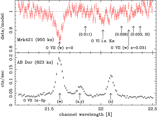
Figure 1: The deep (955 ksec) absorption spectrum toward Mrk 421 (top panel). Locations for intervening absorption features previously reported by Nicastro et al. (2005b) are indicated with parenthesized redshifts. The Mrk 421 spectrum is given alongside a line–rich coronal spectrum (bottom panel) of comparable integration time and observation count for comparison. Both plots use the instrument’s blind wavelength scale for their constituent datasets. The O VII $w$ emission line profile in the spectrum of AB Dor provides a model- and calibration-independent estimate for the effective wavelength response in spectra composed of many different datasets.

Each data set generated was then analyzed in parallel within XSPEC (Arnaud 1996) as a separate spectrum paired with its specific response matrix and backlight emission model. A total of 10 isolated channels (out of a total 2268) stood out by contributing $\Delta\chi^{2}>10$ and were excluded from the fit. Indeed, 8 of these 10 channels reside in the 6 datasets with the susceptibility parameter $S>0.025$′ (cf. Tab. 2), consistent with some of our initial considerations on systematic errors.

The spectra of all the data sets included in the joint fit are combined only for plotting purposes via XSPEC’s setplot group command. The resulting absorption spectrum is given in Figure 1, where each spectrum was divided through by its specific folded powerlaw continuum model prior to averaging across data sets. In the following section we discuss the quantitative analysis of this composite spectrum representing 955 ks of integration time toward Mrk 421.

4 Analysis of the 21.2–22.5Å spectrum

4.1 Continuum modeling; the discrete absorption at redshift zero

The absorption spectrum in the range where the O VII $w$ line should appear for the redshift range $z=0-0.030$ was generated as described above. No additional splines to the instrument response were applied, so any uncorrected, differential calibration errors over this spectral range will appear in these residuals. We neglected any absorption by neutral gas in our Galaxy in the fitting, since our analysis spans a narrow wavelength band. The foreground column density is small ($N_{\mathrm{H}}=1.61\times 10^{20}$ cm^-2, Lockman & Savage 1995), and the transmission $T$ of the ISM varies by 2% across the chosen range, but can be approximated locally by a power law $T\sim\lambda^{-0.38}$ within 0.02 % accuracy. The most prominent absorption features ($\lambda=21.6,\,22.0$ Å) were fitted at the same time, but the wavelength and strength were fixed across all data sets because the absorber is considered to be independent of the backlight spectrum. Our method therefore reduces any differences in the continuum between data sets.

Next, absorption parameters for each line feature were further determined by fitting only in a narrow spectral range centered on each feature. The powerlaw indices of each data set (determined by fitting over $21.3<\lambda<22.5$ Å) were held fixed and only their normalizations were allowed to vary. The fitting ranges were ($21.4<\lambda<21.8$ Å), ($21.9<\lambda<22.1$ Å) and ($22.2<\lambda<22.4$ Å), respectively, for the three detected features listed in Table 3.

Table 3: Joint fitting results and line detection limits for datasets in Table 2

Feature	$\lambda_{meas}$	$\Delta\lambda$	ID	z	$\rm W_{\lambda}$	$\rm S/N$	$\rm Log\,N_{i}$	$\chi_{\nu}^{2}$(d.o.f.)
1	21.595	${}^{+\phantom{0}3.2}_{-\phantom{0}3.0}$	O VII	$\equiv 0$	$13.6^{+1.1}_{-1.1}$	25.6(20.4)	$15.763^{+0.031}_{-0.046}$	0.951(726)
2	22.022	${}^{+10.0}_{-10.0}$	O VI	$0.0004\pm.0005$	$3.3^{+1.5}_{-1.4}$	6.30(4.2)	$15.22^{\phantom{0}+0.16}_{\phantom{0}-0.23}$	0.902(332)
3	22.290	${}^{+21.1}_{-19.9}$	(O VII)	$0.0318\pm.0010$	$2.1^{+1.4}_{-1.3}$	4.00(2.6)	$14.93^{\phantom{0}+0.43}_{\phantom{0}-0.22}$	1.190(347)
Non–detections
	$\lambda_{input}$	$\Delta\lambda$	ID	z	$\rm W_{\lambda}$		$\lceil\rm Log\,N_{i}\rceil$	$\chi_{\nu}^{2}$(d.o.f.)
$\cdots$	21.85	${}^{+20}_{-20}$	(O VII)	$0.011^{+.001}_{-.001}$	$\phantom{0}0\phantom{0}^{+1.8}_{-1.4}$	$\cdots$	14.78(15.01)	1.025(346)
$\cdots$	22.20	${}^{+20}_{-20}$	(O VII)	$0.028^{+.001}_{-.001}$	$\phantom{0}0\phantom{0}^{+2.0}_{-1.2}$	$\cdots$	14.81(15.06)	1.229(347)
$\cdots$	22.32	${}^{+20}_{-20}$	(O VII)	$0.033^{+.001}_{-.001}$	$\phantom{0}0\phantom{0}^{+2.7}_{-0.5}$	$\cdots$	14.93(14.93)	1.182(348)

To fit absorption line profiles and to estimate equivalent widths, we generated response matrices with energy bin densities that oversample the RGS spectral resolution by a factor of about 5 ($\Delta\lambda\sim\lambda/1800$), sufficient to model narrow features in the spectra. For the intrinsic line profiles we used the Voigt profile, evaluated appropriately for a discrete model wavelength grid.

The fit parameters providing the best fits (for given temperature, atomic mass and Doppler parameter) are given in the oscillator strength–column density product ($fN_{i}$) and the equivalent width $W_{\lambda}$ for the line (again, computed on the spectral model grid).

Three apparent absorption features stand out visually: at wavelengths $\lambda\approx 21.60,22.02,22.29$ Å. The results of formally fitting these features are summarized in the first three entries of Table 3.

The strongest line is identified with the the O VII $w$ transition at $z=0$ (21.602 Å). The best fit wavelength is off by 7 mÅ (or 100 km s^-1) from the expected value and formally outside of the measured 90 % confidence limit range, by 4 mÅ; however this mismatch is smaller than the overall wavelength scale zero point uncertainty. Therefore we assume that it is the 21.602 Å line feature at $z=0$, and it provides a local wavelength fiducial for the remaining features in the spectrum.

The next strongest line is coincident with the dominant inner shell excitation doublet of O VI, also at $z=0$, which has a laboratory wavelength of 22.0194$\pm$0.0016 Å (Schmidt et al. 2004). This line is also quite prominent in Figure 1. The measured strength of this line ($W_{\lambda}\sim 3.3$ mÅ) is marginally consistent with the Chandra LETGS measurement of $2.4\pm 0.9$ mÅ (Williams et al. 2005) but the inferred column density raises some concern, because it is large compared to the column density in O VI resolved by FUSE (Savage et al. 2005). The narrow feature immediately to the right of the O VI inner shell feature appears to be narrower than the instrumental resolution. The source of this fluctuation could be instrumental, but an exhaustive search for its origin has not been performed. Unfortunately the wavelength range is only covered by RGS1 and an independent cross check on this feature is not available.

Finally, the weakest, $\sim 2\sigma$ feature close to 22.29 Å is suggestive of absorption by O VII 21.602 Å in the host galaxy ($0.031<z<0.033$). The 90% confidence range for the feature redshift is marginally consistent with a currently accepted redshift of $z=0.0308$ for Mrk 421 (Ulrich et al. 1975). They did not give an accuracy estimate for their redshift but an inspection of their published plot suggests it may be of the order of 0.001.

4.2 Weak line feature search

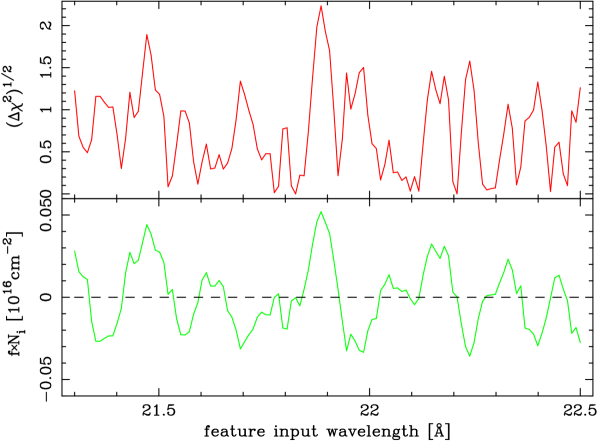
Figure 2: Results of the search for narrow, unresolved features in the O VII region of the spectrum. The positive detections identified in Table 3 have been included in the underlying model. The top plot shows $\sqrt{\Delta\chi^{2}}$ (in units of $\sigma$) between the best fit local continuum level and adding in a line–like feature at the center of the data band where the fitting was performed. The bottom plot gives the best fit parameter $fN_{i}$ which encodes the polarity and equivalent width of the best fit feature.

To identify any other possible spectral features in the wavelength range of interest, we have performed a search by fitting for lines within localized spectral ranges. The fitting ranges were 4 resolution elements in width (0.2 Å) and were centered on the hypothetical feature wavelength. Allowing only the normalizations of the local continua to vary and with the powerlaw indices fixed, the narrow spectral range was fitted. Then a line feature (either in absorption or emission) was introduced to the model and its best fit amplitude was determined, along with the change in $\chi^{2}$. This process was performed on a fine, uniformly spaced grid of wavelengths within the search region. Results of this process are given in Fig. 2. The search is effectively a localized test of the null hypothesis (no line), performed over the spectral range. While some features appear to be fit with significances of 2$\sigma$, the overall distribution of these “detections” is well behaved (Fig. 3) and the number of 2$\sigma$ detections is not greater than expected, according to the $\chi^{2}$ and $F$ distributions. The typical null hypothesis probability for obtaining our value for $F$ is 8.5%. We conclude that at the working sensitivity level of the blind search, the data are consistent with no excess in features above the 2$\sigma$ level (1.9 mÅ; $N_{OVII}\sim 7\times 10^{14}$ cm^-2) that may trace intervening WHIM toward Mrk 421.

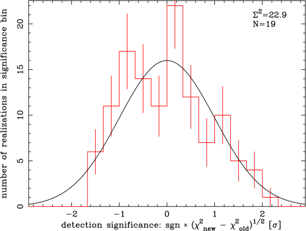
Figure 3: The distribution of “detections” in the narrow feature search results (cf. Fig. 2). The distribution appears to be consistent with what is expected, based on the $\chi^{2}$ and $F$ distributions (the overplotted curve). There is no indication for additional intervening absorption systems at this effective sensitivity level ($\sigma$ corresponds to $\delta W_{\lambda}\sim 0.95\,$mÅ).

5 Comparison to Published Results

5.1 Comparison to Williams et al. (2005)

We immediately notice that our measured $W_{\lambda}$ values are significantly larger ($\gtrsim$30%) than those tabulated based on the Chandra results. We investigated reasons for this, and found that the discrepancy is most likely due to the combined effect of several factors. First, it should be noted that $W_{\lambda}$ values derived from order-unsorted data (LETG/HRC-S) can depend strongly on properties of the underlying continuum model and the assumed column density. When we fit the LETGS data ourselves (Kaastra et al. 2006), we obtain $W_{\lambda}$ values for the order sorted (LETG/ACIS-S) observations that exceed the published (Williams et al. 2005) values by roughly 20%. Moreover, when we attempt to estimate $W_{\lambda}$ values graphically from their Figure 1(c) we are able to reproduce their tabulated values precisely. We found this surprising because the presence of spectral contamination in their composite data set (estimated at about 20%) should reduce the apparent $W_{\lambda}$ value correspondingly. We therefore believe that contaminating contributions to the continuum level had not been properly subtracted prior to their $W_{\lambda}$ estimation, thereby resulting in systematically low equivalent widths. Because the discussion of their data analysis refers to Nicastro et al. (2005b) for a thorough description, we infer that the systematic underestimation affects both of these papers.

The presence of finite spectral contamination by scattering further decreases apparent equivalent widths. While integrated contributions of this sort are considered small, we note that off-diagonal terms are neglected in off–the–shelf Chandra matrices: Response values (e.g., http://asc.harvard.edu/cal/Links/Letg/User/Hrc_QE/ea_index.html) are identically zero for off–diagonal elements where $|m\Delta\lambda|>75\rm\,m\AA$.

On the RGS side, it is certainly conceivable that estimated $W_{\lambda}$ values may be systematically high or low by a relatively small ($\sim$10%) amount. Pre-flight calibration activities included illuminating individual RGS gratings to measure their scatter distribution over various angular scales. Interpretation of the raw data naturally placed upper limits to true scatter contributions, but improper accounting for of any spectral contamination in the source or scatter in the beamline each affect the apparent scatter amplitude off of the gratings. A modest overestimation in the grating scatter amplitude in the RGS physical model also lead to overestimates in $W_{\lambda}$ measures, according to our method, by approximately the same amount.

It is evident, therefore, that the $z$=0 O VII feature in the spectrum is reported inconsistently in units of mÅ. Unless otherwise noted in the following discussion, we disregard this fact and use tabulated entries for absorption line strengths ($W_{\lambda}$) taken at face value.

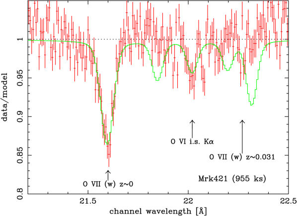
Figure 4: A comparison of the 955 ks absorption spectrum toward Mrk 421 to the absorption line pattern of the Chandra LETGS spectrum (Nicastro et al. 2005b; Williams et al. 2005).

5.2 Comparison to Nicastro et al. (2005b)

As we have already shown above, a blind search of the RGS spectrum for narrow absorption lines in the $21.3-22.5$ Å wavelength range yields no evidence for the presence of lines that could indicate absorption by intervening WHIM. Furthermore, directly fitting for the absorption features identified in the Chandra LETGS spectrum reported by Nicastro et al. (2005b) yielded only null results (cf. the three non–detections tabulated in Table 3).

We are left to compare the XMM-Newton RGS absorption spectrum toward Mrk 421 we obtained to the folded spectrum that is consistent with the reported intervening absorbers. This is given in Figure 4. To generate this comparison we took the feature equivalent widths tabulated in the two LETGS papers (Nicastro et al. 2005b; Williams et al. 2005) together with a quantitative estimate for the $z=0.033$ feature which was not tabulated in either paper, to produce a pattern of absorption features. The pattern amplitude was then scaled to obtain agreement between the data and the folded model for the O VII $w$ ($z=0$) feature as given in Table 3.

The comparison between the RGS data and the synthesized LETGS model (folded through the RGS response) is striking. Overall, two features are in reasonable agreement, while three features are not. All three features that are inconsistent are the purported intervening O VII $w$ absorption systems at redshifts $z\approx$0.011, 0.027 & 0.033. Their presence, at the contrast seen in the LETGS spectrum is ruled out at the 3.5 $\sigma$, 2.8 $\sigma$ and 5.2 $\sigma$ levels, respectively. We can conclude that the features in the Chandra data as reported by Nicastro et al. (2005b) are in disagreement with the results of our analysis of the RGS data.

5.3 Comparison to Williams et al. (2006)

Williams et al. (2006) searched for the z$>0$ absorption lines in a subset of RGS data. They attributed their inability to confirm the intervening WHIM features discovered by Nicastro et al. (2005b) to a host of instrumental problems intrinsic to the RGS, and declared their non-detection fully consistent with the Chandra measurement. We have demonstrated that a careful analysis is not in agreement with this conclusion. We have successfully used the XMM-Newton RGS to produce and analyze data sets that are minimally affected by instrumental systematics. Our strong exclusion of only the redshifted features detected by Chandra makes the claim for the discovery of the WHIM dubious.

By studying the analysis approach described in Williams et al. (2006), we have ascertained that they introduced certain problems in the method for co-adding the 14 observations. For a source as variable as Mrk 421, where the spectra are accumulated from a large number of pointings characterized by small offsets, certain systematics will naturally be introduced into the data wherever bad detector regions exist. The key lies in understanding how non–continuous detector coverage can be used to still yield results that are not riddled with artifacts from that coverage. Because the countrates in the RGS varied by as much as a factor of 4 for the observations they used, a single bad column that was properly ignored in the data pipeline (but improperly compensated for in modeling) can conceivably introduce multi-modal features with equivalent widths as large as 6 mÅ. This is a factor of 10 or so greater than the 1 $\sigma$ counting statistics limit.

While we accumulated counting statistics to a different level (26000 vs. their 12500 cts per 50 mÅ), this fact alone should have had an inconsequential impact on the overall sensitivity to spectral features of the significance detected by Chandra LETGS. We suggest that Williams et al. (2006) did not exercise proper care in collecting up large quantities of data for the purpose of measuring faint spectral features.

Irrespective of our mutually opposing conclusions, secondary reasons for obtaining different quality spectra using the RGS exist, and we list them here:

1. Our data were not added together, but fitting residuals were averaged for display purposes. Each dataset was analyzed with its corresponding response matrix, as described above. This naturally led to nearly complete spectral coverage over the range of interest.

2. Large countrate fluctuations ($\sim$5%) from channel to channel are seen in their spectrum (their Fig. 1), and are suggestive of aliasing problems. Similar fluctuations are sometimes seen only in the longest wavelength range of the RGS and are a result of an overzealous hot pixel finder. The problem can be ameliorated significantly by altering the extraction region definitions or parameters of the hot pixel finder. The problem is normally not noticeable in the shorter wavelength ranges ($\lambda\lesssim 29$Å). The fluctuations seen in all wavelength ranges of their spectrum are therefore suggestive of a different problem. Instead, they are probably due to the co–adding approach they took, which we referred to above.

3. They state that pointing offsets exceeding 15″ were not included because spectral resolution is degraded there. This an unnecessary restriction that led to smaller counting statistics for them. For example, we have combined data from multiple offset pointings, and rely on the aspect correction algorithms for the RGS to align spectral data. The RGS spectral resolution does not really degrade significantly even with $\sim$few arcminute scale pointing offsets.

4. They claim that the presence of a ‘detector feature’ rendered the $z\sim$0.011 feature unmeasurable in the RGS. The SAS provides means to exclude specific detector regions, both from the data and from the response. We have shown that with proper care, systematics arising from detector regions may be almost completely removed. The machinery that provides this capability is available and is central to the RGS branch of the SAS.

We summarize our disagreement with Williams et al. (2006) as follows: While the systematics introduced by their method hindered spectral interpretation, those problems are not insurmountable. Signatures of systematics can be distinguished from instrumental PSFs, and the equivalent widths of the features reported by Nicastro et al. (2005b) are large enough to see by overplotting the data (cf. Fig. 4). As we have demonstrated above, the RGS data can indeed be used to confirm or deny presence of the weak spectral features that constitute the Chandra LETGS (Nicastro et al. 2005b) detections.

6 Conclusions

We have analyzed a very deep spectrum of Mrk 421 obtained with the RGS on XMM-Newton. In 1 Ms of exposure, we collected over 26000 counts per 50 mÅ resolution element,which gives us high sensitivity to the detection of narrow absorption lines. We describe the detailed procedure by which we reduced the data, which results in a continuum spectrum with noise properties that are dominated by statistical fluctuations. The deep continuum spectrum of Mrk 421 is well enough understood that it allows us to detect real absorption lines of equivalent width $>2.4$ mÅ with 99% confidence.

Focusing attention on the $21.3-22.5$ Å band, which contains the wavelength range in which intervening O VII $w$ absorption lines along the line of sight to Mrk 421 should be contained, we find no evidence for redshifted absorption lines. We place a 2 $\sigma$ upper limit of 1.9 mÅ on the equivalent with of any narrow absorption line over the quoted wavelength band.

This finding is in clear conflict with the claim of the detection of narrow absorption lines at 21.85 and 22.20 Å in the deep Chandra LETGS spectrum of the source, which would naturally correspond to O VII $w$ lines redshifted to $z=0.011$ and $z=0.027$, respectively. We find that absorption lines at these positions, at the equivalent widths claimed on the basis of the Chandra LETGS spectrum, are excluded with high confidence (3.5 and 2.8 $\sigma$, respectively). The exclusion becomes only stronger when we use the mutually detected O VII $z=0$ feature as an absorption fiducial to align the $W_{\lambda}$ values measured across instruments as represented in Figure 4 (5.3 and 3.8 $\sigma$, respectively).

We conclude that the detection of absorption by intergalactic He-like oxygen in filaments of column densities $N_{i}\approx 8.5\times 10^{14}$ cm^-2 is all but excluded (with 99% confidence) by our data. Possible explanations for the apparent discrepancy between the XMM-Newton and Chandra spectroscopic results are investigated in an accompanying paper (Kaastra et al. 2006).

The non-detection of intervening absorption, even in the deepest exposures that can currently be contemplated, on the brightest suitable extragalactic continuum source, is probably not surprising. The redshift of Mrk 421 is relatively small, and the a priori probability, as predicted by recent cosmological gas dynamics simulations, of having an intervening filament with a column density that is readily and convincingly detectable with the current instrumentation, is relatively small: for $Z\sim 0.1\,Z_{\sun}$, ${dP\over dz}\times z_{Mrk421}\sim 0.05-0.2$ for Log$(N_{i})>15.0$ and $14.6$, respectively (Fang et al. 2002a; Chen et al. 2003). The most uncertain parameter in these calculations is the absolute oxygen abundance, which can currently not be calculated with confidence from first principles. The null detections therefore do not yet constrain these calculations in a meaningful way. The detection of the ‘missing baryons’ remains a challenge, best addressed with higher resolution, higher sensitivity spectrometers.

Appendix A Effects of removing detector regions

A demonstration of the iterative analysis approach is given here. The data in Figure 5 is from the dataset 0720, and is plotted in terms of its ratio to a folded model. The top histogram is the data processed with automatic detection and rejection of flickering pixels, divided through with a continuum model folded through its corresponding response matrix. An instrumental, sharp feature located close to 21.8Å, is identified with equivalent width roughly 2.5 mÅ. Inspection of the same data binned by hardware address reveals a single column with non–standard response. Because the RGS normally operates in 3$\times$3 on–chip binning (OCB) mode, the charge healthy and unhealthy columns alike are added prior to digitization. In this case, it appears that the charge from a single unhealthy column is added to the charge of two healthy ones prior to signal readout. The middle panel shows the same data after reprocessing, where the channel in question was rejected. As a test of this method, we have also manually rejected an additional randomly selected CCD column whose absense is seen at a channel wavelength of $\sim$21.37Å. These data are divided by the same folded model and response matrix as in the top panel. The rejected column affects more than one spectral channel because of the chosen bin size. The bottom histogram finally shows the same data as in the middle, but here is divided through by the folded model using the updated response matrix, which include effects of the rejected columns. While the column rejection process appears to introduce some minor artifacts, substantial reduction in incidence of non-statistical outliers is seen.

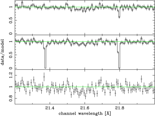
Figure 5: A demonstration of removing detector regions in the data reduction process. A column with non-standard response (close to 21.8Å) is rejected, along with a typical, randomly selected column (close to 21.37Å). The three spectra depict the same data at different iterations of the reduction.

Appendix B Weak spectral features arising from systematics

We have shown above that with careful data analysis techniques, including identification of problematic detector locations, systematics can be reduced to a level which is comparable to the statistical limit. As statistics build up in very deep, large signal–to–noise observations, beating down systematics is critical in order for a proper identification of weak features.

The section of the spectrum discussed in this paper is recorded on a single CCD in RGS1 which, due to a CCD failure early in the mission, has no counterpart in RGS2. The quality of this CCD will be comparable to other CCD’s on the RGS so the comparison between RGS1 and RGS2 can give us a model independent estimate of the magnitude of systematic effects which may be present in RGS spectra in general and in the section of the spectrum analyzed in this paper in particular.

To evaluate remaining systematic errors in RGS we have performed a model independent analysis of the source spectrum seen by the twin RGS instruments. By comparing the count ratio seen by the two instruments on a channel–by–channel basis in wavelength coordinates and comparing this to an expected statistical distribution, the non–statistical (or systematic) contribution may be resolved from the statistical population as a wing. Figure 6 displays an example of this distribution, with a Gaussian distribution (based on the channel counts only) overlaid to guide the eye and to help visualize the non–statistical contribution.

Table 4 provides a tabulation of these quantities for bins of 40 mÅ  (the approximate width of the RGS PSF) per CCD pair. Based on these results if one only assumes purely statistical errors, there is about a 15% chance of falsely identifying a feature. For $>2\sigma$ features this corresponds to 3 mÅ  absorption features. It is stressed that the type of systematics discussed here can only result in absorption features and not in emission features, since all these effects can only lower the effective area and not increase it.

Among the main causes for the non-statistical distribution in Figure 6 will be the effects of small differences in CTE between columns in relation to the pulse-height data selection window. Columns with clearly bad CTE will be manually discarded, but small CTE differences may not be recognized. They will however, influence the number of recorded photons due to the pulse-height selection window and hence will result in non-statistical count rate differences.

Recognition of individual systematic features, which are linked to fixed detector positions, can only be done with high confidence if detector coordinates change over time with respect to the wavelength coordinates i.e. an effective dithering of the observations. In addition, systematic features too weak to be recognized will be smeared-out by dithering, effectively decreasing their impact. It would therefore be advisable to purposely dither long RGS observations when detection of weak spectral features is desired.

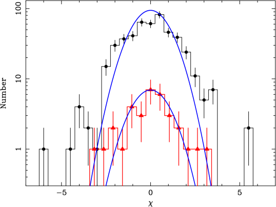
Figure 6: The difference between RGS1 and RGS2, based on background subtracted counts. The (top) histogram (filled circles) shows count differences for single spectral bins between the two RGS spectrometers, divided by the computed statistical variance of the difference. The non–Gaussian tail component is assumed to be the non–statistical, systematic contribution. The overplotted continuous line, for comparison purpose, shows a strict Gaussian distribution, based on count statistics only. The lower distribution (filled triangles) show the distribution of differences between the model continuum and the actual data for the analyzed section of RGS1, CCD4; the CCD which is used to obtain the spectrum section discussed in this paper. Since this spectrum contains a spectral range of only $\sim$1.2Å, compared to the overlapping coverage between RGS1 and RGS2 ($\sim$21Å), there is a factor of about 15 difference in number of data points binned. The actual distributions appear indeed to be shifted with respect to each other by a constant factor of about 10, confirming that our estimate of systematic errors can also be applied to the section of the spectrum discussed here.

Table 4: Consistency between RGS1 and RGS2 showing only those CCD’s which are operational in both RGSs. The flux and noise columns indicate the flux and statistical noise in the Mrk 421 spectrum for the specified CCD. $W_{\lambda}$ gives the equivalent width of a 1 $\sigma$ feature. The last column indicates what percentage of the data lies outside the statistical Gaussian distribution. These results indicate that there is an overall probability of about 15% for a $2\sigma$ feature with a typical EW of 3 mÅ, when the data is sampled for 40 mÅ bins.

CCD	Flux	Noise	$W_{\lambda}$	Outside
	s-1 cm-2	s-1 cm-2	mÅ	%
1	0.0100	0.0004	1.55	5
2	0.0105	0.0004	1.48	12
3	0.0122	0.0005	1.59	14
-
5	0.0140	0.0003	0.83	12
6	0.0145	0.0003	0.80	20
-
8	0.0140	0.0004	1.11	25
9	0.0130	0.0007	2.09	20

Appendix C SAS data reduction prescriptions

Almost all XMM observers use the standard XMM software (SAS) for their analysis. We describe in this section how we processed the Mrk 421 observations using the SAS and dealt with the systematic effects present in the data.

The SAS does handle some aspects of CCD systematics by default, but some others require manual control. This is only relevant in the search of weak features in spectra with a rather long observations. We used the SAS version 6.5, but with task ‘rgsenergy’ version 2.0.3 (standard SAS version 6.5 uses ‘rgsenergy’ version 2.0.2). This allows CCD-pixel dependent offsets to be subtracted (option: withdiagoffset=yes). These offsets are retrieved from diagnostics CCD images, sampled at regular intervals during observations. In addition, the default filter in the SAS to recognize and delete hot pixels was modified to delete the hot pixels only, and not their neighbors (option: rejflags=”BAD_SHAPE ON_BADPIX ON_WINDOW_BORDER BELOW_ACCEPTANCE” ).

The SAS removes detectable, high duty cycle (“hot”) pixels by default. To identify additional bad pixels and columns not recognized by the SAS, the data are displayed in the CCD coordinate reference frame as images of photon energy versus the CCD dispersion axis. Since the individual Mrk 421 observations have slightly different pointings, real spectral features are spread out over a range of CCD hardware coordinates, while CCD defects are localized in these coordinates. Such displays were used to identify local CCD defects. Using software written for this purpose, suspicious columns and pixels are found manually and included in the SAS current calibration files (CCF) to be removed during the subsequent processing. As described in the text, many of the columns identified in this way seem to suffer from loss of charge transfer presumably due to local CCD radiation damage. In the Energy versus CCD-column plot, X-ray events appear to be recorded at much lower energies than for the neighboring columns - resulting in a different detection efficiency into the local pulseheight window. Such regions can currently only be identified manually, with the aid of high counting statistics observations, such as those used here. After modifying the CCF to include these bad columns, all data are processed again through the SAS.

The spectra generated for each individual observation were run through the task rgsfluxer to obtain individually fluxed spectra. Due to the source variability these spectra were not simply added. Instead the spectra are all normalized over a short wavelength interval and these normalized spectra are added. The error is calculated taking into account the normalization.

The final spectrum obtained in this way, using the SAS, appears to be equivalent to the spectrum obtained in our custom analysis. This can be seen in Figure 7.

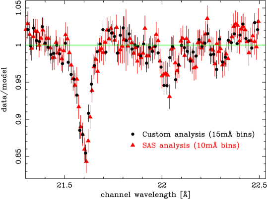
Figure 7: Comparison between the spectrum obtained via the XMM SAS analysis package and our custom software. Binning is slightly different and each package identifies slightly different occasional bad pixels. Nevertheless, the spectra obtained are practically identical.

References

- Arnaud (1996) Arnaud, K. A. 1996, in ASP Conf. Ser. 101: Astronomical Data Analysis Software and Systems V, ed. G. H. Jacoby & J. Barnes, 17–+
- Barcons et al. (2005) Barcons, X., Paerels, F. B. S., Carrera, F. J., Ceballos, M. T., & Sako, M. 2005, MNRAS, 359, 1549
- Brinkman et al. (2000) Brinkman, B. C., Gunsing, T., Kaastra, J. S., van der Meer, R., Mewe, R., Paerels, F. B., Raassen, T., van Rooijen, J., Braeuninger, H. W., Burwitz, V., Hartner, G. D., Kettenring, G., Predehl, P., Drake, J. J., Johnson, C. O., Kenter, A. T., Kraft, R. P., Murray, S. S., Ratzlaff, P. W., & Wargelin, B. J. 2000, in Proc. SPIE Vol. 4012, p. 81-90, X-Ray Optics, Instruments, and Missions III, Joachim E. Truemper; Bernd Aschenbach; Eds., ed. J. E. Truemper & B. Aschenbach, 81–90
- Burles & Tytler (1997) Burles, S., & Tytler, D. 1997, AJ, 114, 1330
- Burles & Tytler (1998) —. 1998, ApJ, 507, 732
- Cagnoni et al. (2004) Cagnoni, I., Nicastro, F., Maraschi, L., Treves, A., & Tavecchio, F. 2004, ApJ, 603, 449
- Canizares et al. (2000) Canizares, C. R., Huenemoerder, D. P., Davis, D. S., Dewey, D., Flanagan, K. A., Houck, J., Markert, T. H., Marshall, H. L., Schattenburg, M. L., Schulz, N. S., Wise, M., Drake, J. J., & Brickhouse, N. S. 2000, ApJ, 539, L41
- Cen & Ostriker (1999) Cen, R., & Ostriker, J. P. 1999, ApJ, 514, 1
- Chen et al. (2003) Chen, X., Weinberg, D. H., Katz, N., & Davé, R. 2003, ApJ, 594, 42
- Cowie et al. (1995) Cowie, L. L., Songaila, A., Kim, T.-S., & Hu, E. M. 1995, AJ, 109, 1522
- Croft et al. (2001) Croft, R. A. C., Di Matteo, T., Davé, R., Hernquist, L., Katz, N., Fardal, M. A., & Weinberg, D. H. 2001, ApJ, 557, 67
- den Herder et al. (2001) den Herder, J. W., Brinkman, A. C., Kahn, S. M., Branduardi-Raymont, G., Thomsen, K., Aarts, H., Audard, M., Bixler, J. V., den Boggende, A. J., Cottam, J., Decker, T., Dubbeldam, L., Erd, C., Goulooze, H., Güdel, M., Guttridge, P., Hailey, C. J., Janabi, K. A., Kaastra, J. S., de Korte, P. A. J., van Leeuwen, B. J., Mauche, C., McCalden, A. J., Mewe, R., Naber, A., Paerels, F. B., Peterson, J. R., Rasmussen, A. P., Rees, K., Sakelliou, I., Sako, M., Spodek, J., Stern, M., Tamura, T., Tandy, J., de Vries, C. P., Welch, S., & Zehnder, A. 2001, A&A, 365, L7
- Fang et al. (2002a) Fang, T., Bryan, G. L., & Canizares, C. R. 2002a, ApJ, 564, 604
- Fang & Canizares (2000) Fang, T., & Canizares, C. R. 2000, ApJ, 539, 532
- Fang et al. (2001) Fang, T., Marshall, H. L., Bryan, G. L., & Canizares, C. R. 2001, ApJ, 555, 356
- Fang et al. (2002b) Fang, T., Marshall, H. L., Lee, J. C., Davis, D. S., & Canizares, C. R. 2002b, ApJ, 572, L127
- Kaastra et al. (2006) Kaastra, J. S., Werner, N., den Herder, J. W. A., Paerels, F. B. S., de Plaa, J., & Rasmussen, A. P. de Vries, C. P. 2006, ApJ, (submitted)
- Mathur et al. (2003) Mathur, S., Weinberg, D. H., & Chen, X. 2003, ApJ, 582, 82
- Nicastro et al. (2001) Nicastro, F., Fruscione, A., Elvis, M., Siemiginowska, A., Fiore, F., & Bianchi, S. 2001, in ASP Conf. Ser. 234: X-ray Astronomy 2000, ed. R. Giacconi, S. Serio, & L. Stella, 511–+
- Nicastro et al. (2005a) Nicastro, F., Mathur, S., Elvis, M., Drake, J., Fang, T., Fruscione, A., Krongold, Y., Marshall, H., Williams, R., & Zezas, A. 2005a, Nature, 433, 495
- Nicastro et al. (2005b) Nicastro, F., Mathur, S., Elvis, M., Drake, J., Fiore, F., Fang, T., Fruscione, A., Krongold, Y., Marshall, H., & Williams, R. 2005b, ApJ, 629, 700
- Nicastro et al. (2002) Nicastro, F., Zezas, A., Drake, J., Elvis, M., Fiore, F., Fruscione, A., Marengo, M., Mathur, S., & Bianchi, S. 2002, ApJ, 573, 157
- Paerels et al. (2003) Paerels, F., Rasmussen, A., Kahn, S., Herder, J. W., & Vries, C. 2003, X-ray Absorption and Emission Spectroscopy of the Intergalactic Medium at Small Redshift
- Rasmussen et al. (2003a) Rasmussen, A., Kahn, S. M., & Paerels, F. 2003a, in ASSL Vol. 281: The IGM/Galaxy Connection. The Distribution of Baryons at z=0, ed. J. L. Rosenberg & M. E. Putman, 109–+
- Rasmussen et al. (2003b) Rasmussen, A., Kahn, S. M., Paerels, F., den Herder, J., & de Vries, C. 2003b, AAS/High Energy Astrophysics Division, 7, #201
- Ravasio et al. (2005) Ravasio, M., Tagliaferri, G., Pollock, A. M. T., Ghisellini, G., & Tavecchio, F. 2005, A&A, 438, 481
- Savage et al. (2005) Savage, B. D., Wakker, B. P., Fox, A. J., & Sembach, K. R. 2005, ApJ, 619, 863
- Schmidt et al. (2004) Schmidt, M., Beiersdorfer, P., Chen, H., Thorn, D. B., Träbert, E., & Behar, E. 2004, ApJ, 604, 562
- Ulrich et al. (1975) Ulrich, M.-H., Kinman, T. D., Lynds, C. R., Rieke, G. H., & Ekers, R. D. 1975, ApJ, 198, 261
- Williams et al. (2006) Williams, R. J., Mathur, S., Nicastro, F., & Elvis, M. 2006, ApJ, accepted for publication
- Williams et al. (2005) Williams, R. J., Mathur, S., Nicastro, F., Elvis, M., Drake, J. J., Fang, T., Fiore, F., Krongold, Y., Wang, Q. D., & Yao, Y. 2005, ApJ, 631, 856