Hot Accretion With Conduction: Spontaneous Thermal Outflows

Abstract

Motivated by the low-collisionality of gas accreted onto black holes in Sgr A* and other nearby galactic nuclei, we study a family of 2D advective accretion solutions with thermal conduction. While we only impose global inflow, the accretion flow spontaneously develops bipolar outflows. The role of conduction is key in providing the extra degree of freedom (latitudinal energy transport) necessary to launch these rotating thermal outflows. The sign of the Bernoulli constant does not discriminate between inflowing and outflowing regions. Our parameter survey covers mass outflow rates from $\sim 0$ to $13\%$ of the net inflow rate, outflow velocities from $\sim 0$ to $11\%$ of the local Keplerian velocity and outflow opening angles from $\sim 0$ to $60$ degs. As the magnitude of conduction is increased, outflows can adopt a conical geometry, pure inflow solutions emerge, and the limit of 2D non-rotating Bondi-like solutions is eventually reached. These results confirm that radiatively-inefficient, hot accretion flows have a hydrodynamical propensity to generate bipolar thermal outflows.

1 Introduction

Over the past decade, X-ray observations have made it increasingly clear that black holes are capable of accreting gas under a variety of flow configurations. In particular, there is convincing evidence that a distinct form of hot accretion exists at sub-Eddington rates, which contrasts with the classical “cold and thin” accretion disk scenario (Shakura & Sunyaev 1973). Hot accretion appears to be common in the population of supermassive black holes in galactic nuclei and during the quiescent phases of accretion onto stellar-mass black holes in X-ray transients (e.g. Narayan et al. 1998a; Lasota et al. 1996; Di Matteo et al. 2000; Esin et al. 1997, 2001; Menou et al. 1999; see Narayan, Mahadevan & Quataert, 1998b; Melia & Falcke 2001; Narayan 2003; Narayan & Quataert 2005 for reviews).

Theories for the structure and properties of hot accretion flows remain controversial, however. Inspired by the work of Shapiro, Lightman & Eardley (1976), Narayan & Yi (1994; 1995a,b) derived self-similar ADAF solutions which emphasized the important stabilizing role of radial heat advection (see also Ichimaru 1977; Rees et al. 1982; Abramowicz et al. 1988). Subsequent analytical work on hot accretion flows has emphasized the possibility of outflows, motivated by a positive Bernoulli constant (Narayan & Yi 1994; ADIOS: Blandford & Begelman 1999), and the potential role of convection (CDAFs; Narayan et al. 2000, Quataert & Gruzinov 2000a). Hydrodynamical and MHD numerical simulations, on the other hand, have greatly contributed to the subject by highlighting important dynamical aspects of the problem which are not captured by idealized analytical models (e.g. Stone et al. 1999; Stone & Pringle 2001; Hawley et al. 2001; DeVilliers et al. 2003; Proga & Begelman 2003; McKinney & Gammie 2004).

The purpose of this work is to consider the possibility that thermal conduction, which has been a largely neglected ingredient, could affect the global properties of hot accretion flows substantially. In §2, we use existing observational constraints on a few nearby galactic nuclei to argue that hot accretion is likely to proceed under weakly-collisional conditions in these systems, thus implying that thermal conduction could be important. In §3, we extend the original 1D self-similar solutions of Narayan & Yi (1994) to include a saturated form of thermal conduction and we study the effects of conduction on the flow structure and properties. In §4, we generalize the 2D solutions of Narayan & Yi (1995a) in the presence of thermal conduction and find that this extra degree of freedom allows the emergence of rotating thermal outflows. In §5, we discuss our results in the context of recently established observational trends for hot accretion flows and related outflows. In §6, we comment on several limitations of our work, potential additional consequences of strong thermal conduction in hot accretion flows as well as directions for future work.

2 Observational Constraints and Collisionality

Chandra observations provide tight constraints on the density and temperature of gas at or near the Bondi capture radius in Sgr A* and several other nearby galactic nuclei. These observational constraints have been used before to estimate the rate at which the gas is captured by the black hole in these systems, following Bondi theory (e.g. Loewenstein et al. 2001; Di Matteo et al. 2003; Narayan 2003). Here, we use these same constraints (taken from Loewenstein et al. 2001; Baganoff et al. 2003; Di Matteo et al. 2003; Ho, Terashima & Ulvestad 2003) to calculate mean free paths for the observed gas. It should be noted that these constraints are not all equally good, in the sense that Chandra has probably resolved the gas capture radius in Sgr A* and M87 but not in the other nuclei.

Galactic nuclei and their associated gas properties on $1^{\prime\prime}$ scales are listed in Table 1: $n_{1^{\prime\prime}}$ is the gas number density, $T_{1^{\prime\prime}}$ is the temperature, $R_{1}$ is the $1^{\prime\prime}$ size-equivalent at the nucleus distance, $l_{1}$ is the mean free path for the observed $1^{\prime\prime}$ conditions and $R_{\rm cap}$ is the capture radius, inferred from the gas temperature and the black hole mass in each nucleus. From Spitzer’s (1962) expressions for collision times, a standard expression for the thermal speed and a Coulomb logarithm $\ln\Lambda\simeq 20$, one gets the simple mean free path scaling $l\simeq 10^{4}(T^{2}/n)$ cm (Cowie & McKee 1997; valid for both electrons and protons in a 1-temperature gas). We have used this relation to calculate $l_{1}$ values in Table 1.

The inferred mean free paths are in the few hundredths to few tenths of the observed $1^{\prime\prime}$ scales ($l_{1}/R_{1}$ values in Table 1). Assuming no change in the gas properties down to the inferred capture radius, values of $l_{1}/R_{\rm cap}\mathrel{\hbox to0.0pt{\lower 4.0pt\hbox{\hskip 1.0pt$\sim$}\hss}\raise 1.0pt\hbox{$>$}}0.1$ are deduced in four of the six nuclei. One could also reformulate these scalings by stating that the $1^{\prime\prime}$ mean free paths are systematically $\mathrel{\hbox to0.0pt{\lower 4.0pt\hbox{\hskip 1.0pt$\sim$}\hss}\raise 1.0pt\hbox{$>$}}10^{4-5}R_{\rm s}$, where $R_{\rm s}$ is the Schwarzschild radius (the typical length-scale associated with the accreting black holes). These numbers suggest that accretion will proceed under weakly-collisional conditions in these systems.

The weakly-collisional nature of ADAFs has been noted before (e.g. Mahadevan & Quataert 1997), in the sense of collision times longer than the gas inflow time, but these are model-dependent statements. Direct observational constraints on the gas properties near the capture radius favor a weakly-collisional regime of hot accretion, more or less independently of the exact hot flow structure. Whether the gas adopts an ADAF, CDAF or ADIOS type configuration once it crosses the capture radius, it is expected to become even more weakly-collisional as it approaches the black hole, since the relative mean free path scales as $l/R\propto R^{-3/2-p}$ in these flow solutions with a virial temperature profile and a density profile $\rho\propto R^{-3/2+p}$.

Tangled magnetic fields in the turbulent accretion flow would likely reduce the effective mean free paths of particles. The magnitude of this reduction, which will depend on the field geometry, is currently unknown. We return to this important issue in our discussion section. Even if the effective mean free paths of electrons are reduced to values $l_{\rm eff}/R\mathrel{\hbox to0.0pt{\lower 3.0pt\hbox{$\mathchar 536\relax$}\hss}\raise 2.0pt\hbox{$\mathchar 316\relax$}}1$, thermal conduction may be important . It is therefore of interest to investigate its effects on the structure and properties of hot accretion flows in general. We begin with a study of 1D ADAF models with conduction in §3 and then move on to study a 2D version of these hot accretion flows in §4.

3 One-Dimensional Hot Accretion Flows with Saturated Conduction

3.1 The Self-Similar Equations in One Dimension

The standard Spitzer formula for thermal conduction applies only to gas well into the collisional (“fluid”) regime, with a mean free path $l\ll L$, for any relevant flow scale $L$. We expect radial temperature variations on scales $\sim R$ from self-similarity. In a weakly-collisional regime with $l\gg R$ or even $l\sim R$, a saturated (or equiv. “flux-limited”) thermal conduction formalism should be adopted if one is to avoid unphysically large heat fluxes. We adopt the formulation of Cowie and McKee (1977) and write the saturated conduction flux as $F_{s}=5\Phi_{\rm s}\rho c_{s}^{3}$, where $\Phi_{\rm s}$ is the saturation constant (presumably $\sim 1$), $\rho$ is the gas mass density and $c_{s}$ is its isothermal sound speed. With this prescription, the largest achievable conduction flux is approximated as the product of the thermal energy density in electrons times their characteristic thermal velocity (assuming a thermal distribution and equal electron and ion temperatures; see Cowie and McKee 1977 for details). Because it is a saturated flux, it no longer explicitly depends on the magnitude of the temperature gradient but only on the direction of this gradient. Heat will flow outward in a 1D hot accretion flow with a near-virial temperature profile, hence the positive sign adopted for $F_{s}$.

With this formulation for conduction, the steady-state 1-temperature self-similar ADAF solution of Narayan & Yi (1994) can be generalized to include the divergence of the saturated conduction flux in the entropy-energy equation (see also Honma 1996 and Manmoto et al. 2000 for investigations of the role of “turbulent” heat transport in one-dimensional ADAF-like flows). Adopting the same cylindrical geometry and notation as Narayan & Yi (1994), we consider a “visco-turbulent”, differentially rotating hot flow which satisfies the following height-integrated equations for the conservation of momentum and energy

$$v_{r}\frac{dv_{r}}{dR} = R(\Omega^{2}-\Omega_{K}^{2})-\frac{1}{\rho}\frac{d}{dR}(\rho c_{s}^{2}),$$ (1)

$$v_{r}\frac{d(\Omega R^{2})}{dR} = \frac{1}{\rho RH}\frac{d}{dR}\left(\frac{\alpha\rho c_{s}^{2}R^{3}H}{\Omega_{K}}\frac{d\Omega}{dR}\right),$$ (2)

$$2H\rho v_{r}T\frac{ds}{dR} = f\frac{2\alpha\rho c_{s}^{2}R^{2}H}{\Omega_{K}}\left(\frac{d\Omega}{dR}\right)^{2}-\frac{2H}{R}\frac{d}{dR}(RF_{s}),$$ (3)

supplemented by the continuity equation, which is rewritten as $\dot{M}=-4\pi RHv_{r}\rho$. The last term in equation (3) is the additional divergence of the saturated conduction flux. In these equations, $R$ is the cylindrical radius, $\Omega_{K}$ is the Keplerian angular velocity around the central accreting mass, $v_{r}$ is the gas radial inflow speed, $\Omega$ is its angular velocity, $\rho$ is the mass density, $c_{s}$ is the isothermal sound speed, $s$ is the gas specific entropy, $T$ is its temperature, $H=Rc_{s}/v_{K}$ is the flow vertical thickness and $f\leq 1$ is the advection parameter ($f=1$ for negligible gas cooling). A Shakura-Sunyaev prescription has been used to capture the “visco-turbulent” nature of the flow, with an equivalent kinematic viscosity coefficient $\nu=\alpha c_{s}^{2}/\Omega_{K}$, where $\alpha$ is the traditional viscosity parameter.

We look for solutions to these equations of the form

$$\rho=\rho_{0}R^{-3/2},~{}v_{r}=v_{0}R^{-1/2},~{}\Omega=\Omega_{0}R^{-3/2},~{}c_{s}^{2}=c_{s0}^{2}R^{-1},$$ (4)

and use the notation $v_{K}=v_{K0}R^{-1/2}=R\Omega_{K}=R\Omega_{K0}R^{-3/2}$. We find that the three unknowns $v_{0}$, $\Omega_{0}$ and $c_{s0}$ satisfy the relations

$$\frac{1}{2}v_{0}^{2} - \Omega_{K0}^{2}+\Omega_{0}^{2}+\frac{5}{2}c_{s0}^{2}=0,$$ (5)

$$v_{0} = -\frac{3\alpha}{2}\frac{c_{s0}^{2}}{v_{K0}},$$ (6)

$$\frac{9\alpha^{2}}{8}c_{s0}^{4} + \left(\frac{5}{2}+\frac{5/3-\gamma}{f(\gamma-1)}\right)c_{s0}^{2}v_{K0}^{2}-\frac{40\Phi_{\rm s}}{9\alpha f}c_{s0}v_{K0}^{3}$$ (7)

$$-v_{K0}^{4}=0,$$

while the density scale, $\rho_{0}$, is fixed by the accretion rate, $\dot{M}$.

Contrary to the original ADAF solution, the energy relation (Eq. [7]) is not a quadratic in $(c_{s0}/v_{K0})^{2}$ because of the extra saturated conduction term. We solve this fourth order polynomial with a standard numerical technique (Press et al. 1992) and discard the two imaginary roots as well as the real root with negative $c_{s0}$, which is unphysical because of a conduction flux going up the temperature gradient.

3.2 Results: Hot Accretion in One Dimension

The main features of the new self-similar solutions with saturated conduction are illustrated in Figure 1, as a function of the value of the saturation constant, $\Phi_{s}$. We are showing results for two distinct solutions here, with $\gamma=1.5$ and $\gamma=1.1$, while we have fixed $f=1$ and $\alpha=0.2$ in both cases. Even though a value of $\gamma<4/3$ may not be physically meaningful, it is useful to illustrate more clearly how solutions depend on $\gamma$.

Original 1D ADAF solutions are recovered at small $\Phi_{\rm s}$ values. As $\Phi_{\rm s}$ approaches unity, however, the solutions deviate substantially from the standard ADAF. The sound speed, $c_{s}$, and the radial inflow speed, $-v_{r}$, both increase with the magnitude of conduction, while the squared angular velocity, $\Omega^{2}$, decreases. Formal solutions still exist when $\Omega^{2}$ becomes negative but they are obviously physically unacceptable. The solution with $\gamma=1.5$ reaches the non-rotating limit at $\log\Phi_{\rm s}\simeq-2$, while the solution with $\gamma=1.1$ reaches this limit for $\log\Phi_{\rm s}\simeq-0.8$. Both solutions have sub-virial temperatures ($c_{s}<v_{k}$) and subsonic radial inflow speeds ($-v_{r}<c_{s}$), which appear to be rather general properties. Supersonic solutions may exist for large $\alpha$ values when $\gamma\to 5/3$.

As the level of saturated conduction is increased, more and more heat flows from the hotter, inner regions, resulting in a local increase of the gas temperature relative to the original ADAF solution. Simultaneously, the gas adjusts its angular velocity (which reduces the level of viscous dissipation) and increases its inflow speed to conserve its momentum balance (increasing at the same time the level of advection). One can show from the energy equation that $\Omega^{2}\propto(1-|q_{\rm cond}/q_{\rm adv}|)$, where $q_{\rm cond}$ and $q_{\rm adv}$ are the magnitudes of the conduction and advection terms: solutions cease to exist once advection balances exactly the heating due to saturated conduction. We have found that variations in the advection parameter, $f$, have relatively minor effects on the solutions, as long as $f$ is not $\ll 1$. The breakdown of the solutions (when $\Omega^{2}\to 0$) occurs at lower values of the saturation constant $\Phi_{\rm s}$ for smaller $\alpha$ and larger $\gamma$ values. Solutions with $\Omega^{2}=0$ can be viewed as Bondi-like solutions with saturated conduction.

Clearly, conduction can significantly affect the structure and properties of hot accretion flows, even at a level well below the saturated flux value (i.e. for $\Phi_{\rm s}\ll 1$). By analogy with the reasoning of Narayan & Yi (1995a) on convection in 2D self-similar ADAF solutions, one might expect conduction to be more important in the polar regions of hot accretion flows than at their equator. To better understand the role of conduction, it is therefore important to study it in a more realistic two-dimensional setting, without height integration.

4 Two-Dimensional Hot Accretion Flows with Thermal Conduction

4.1 The Self-Similar Equations in Two Dimensions

We now extend the analysis of the previous section to two-dimensional hot accretion flows, following closely the methods of Narayan & Yi (1995a). We also discuss in Appendix C the relation between our work and that of Anderson (1987). Adopting spherical polar coordinates ($r\theta\phi$), we consider axisymmetric, steady-state flows ($\partial/\partial\phi=\partial/\partial t=0$). We define Keplerian angular and linear velocities as, respectively,

$$\Omega_{\mathrm{K}} \equiv (GM)^{1/2}r^{-3/2},$$ (8)

$$v_{\mathrm{K}} \equiv \Omega_{\mathrm{K}}r,$$ (9)

and we use the same $\alpha$-prescription as before to describe the visco-turbulent nature of the flow:

$$\nu=\alpha c_{s}^{2}/\Omega_{\mathrm{K}},$$ (10)

where $c_{s}$ is the isothermal sound speed ($c_{s}^{2}\equiv P/\rho$).

The fluid equations obeyed by the visco-turbulent accretion flow are written as follows:

$$\nabla\cdot(\rho{\bf v}) \>=\> 0,$$ (11)

$$({\bf v}\cdot{\bf\nabla}){\bf v} \>=\> -\frac{1}{\rho}{\bf\nabla}P-\Omega_{\mathrm{K}}^{2}{\bf r}+\frac{\alpha c_{s}^{2}}{\Omega_{\mathrm{K}}}\nabla\cdot{\bf\sigma},$$ (12)

$${\bf v}\cdot(T{\bf\nabla}s) \>=\> f\alpha\frac{c_{s}^{2}}{\Omega_{\mathrm{K}}}\left[\frac{1}{2}({\bf\sigma}\cdot{\bf\sigma})-\frac{2}{3}(\nabla\cdot{\bf v})^{2}\right]+\frac{1}{\rho}\nabla\cdot(\lambda\nabla T),$$ (13)

where ${\bf\sigma}$ is the viscous stress tensor (divided by the dynamic viscosity, $\rho\nu$). The notation for the other flow variables is the same as in §3. It should become clear, later on, that our main results are not expected to depend critically on the exact form of the viscous stress tensor adopted. To allow a direct comparison with our results in §3 and for consistency with Narayan & Yi (1995a), we use the same advection parameter $f$ to quantify the cooling efficiency of the flow. We will see, however, that this parameter is in fact ill-defined for solutions with conduction. Fully developed forms of these equations (with a few typos and no thermal conduction term) can be found in Narayan & Yi (1995a).

Contrary to the formulation adopted in §3, we do not write the conduction flux in a saturated form here, but return instead to a traditional form where the flux depends linearly on the local temperature gradient. Justifications for this choice are provided in Appendix A. We adopt a form of the thermal conductivity coefficient which preserves the radial self-similarity of the solutions:

$$\lambda(r)=\lambda_{0}r^{-1}.$$ (14)

Following Narayan & Yi (1995a), we consider separable solutions satisfying

$$v_{r}(r,\theta) =\> v_{\mathrm{K}}(r)\,v_{r}(\theta),$$ (15)

$$v_{\theta}(r,\theta) =\> 0,$$ (16)

$$v_{\phi}(r,\theta) =\> v_{\mathrm{K}}(r)\,\Omega(\theta)\sin\theta,$$ (17)

$$\rho(r,\theta) =\> \rho(\theta)\,r^{-3/2},$$ (18)

$$c_{s}(r,\theta) =\> v_{\mathrm{K}}(r)\,c_{s}(\theta).$$ (19)

In Narayan & Yi (1995a), the $\sin\theta$ in the equivalent of Eq. (17) is missing, in what appears to be a typo. Note that we make the same $v_{\theta}=0$ assumption as Narayan & Yi (1995a).

With these forms, solutions automatically satisfy the continuity equation, Eq. (11). The problem is reduced to a one-dimensional differential system along the polar coordinate, $\theta$. We are left to solve the following four coupled differential equations for the dimensionless variables $v_{r}(\theta),\Omega(\theta),\rho(\theta),$ and $c_{s}(\theta)$:

$$\rho\left(-\frac{1}{2}v_{r}^{2}-\sin^{2}\theta\Omega^{2}\right) \>=\> -\rho+\frac{5P}{2}+\alpha P\left(-v_{r}+\cot\theta\frac{dv_{r}}{d\theta}\right)+\alpha\frac{d}{d\theta}\left(P\frac{dv_{r}}{d\theta}\right),$$ (20)

$$-\sin\theta\cos\theta\rho\Omega^{2} = -\frac{dP}{d\theta}+\alpha\left(v_{r}\frac{dP}{d\theta}+\frac{3}{2}P\frac{dv_{r}}{d\theta}\right),$$ (21)

$$\frac{1}{2}\sin\theta\rho v_{r}\Omega \>=\> \alpha\left[-\frac{3}{4}P\Omega+3\cos\theta P\frac{d\Omega}{d\theta}+\sin\theta\frac{d}{d\theta}\left(P\frac{d\Omega}{d\theta}\right)\right],$$ (22)

$$-\frac{3}{2}\epsilon^{\prime}v_{r} \>=\> \alpha\left\{3v_{r}^{2}+\left(\frac{dv_{r}}{d\theta}\right)^{2}+\sin^{2}\theta\left[\frac{9}{4}\Omega^{2}+\left(\frac{d\Omega}{d\theta}\right)^{2}\right]\right\}$$ (23)

$$\qquad\qquad+\lambda_{0}^{\prime}\frac{1}{P}\left[c_{s}^{2}+\frac{1}{\sin\theta}\frac{d}{d\theta}\left(\sin\theta\frac{dc_{s}^{2}}{d\theta}\right)\right].$$

For convenience, the parameters

$$\epsilon^{\prime} \equiv \frac{1}{f}\epsilon=\frac{1}{f}\frac{5/3-\gamma}{\gamma-1},$$ (24)

$$\lambda_{0}^{\prime} \equiv \frac{1}{f}\lambda_{0},$$ (25)

were introduced in the energy equation (Eq. [23]), where $\gamma\equiv c_{p}/c_{v}$ is the adiabatic index of the gas.

This is a seventh-order differential system of four variables. The three momentum equations (Eqs [20–22]) are identical to those presented in Narayan & Yi (1995a). The energy equation (Eq. [23]) differs in that extra terms corresponding to the radial and polar contributions to heat conduction are now present. This qualitative difference turns out to be crucial in providing the extra degree of energetic freedom necessary for inflow or outflow at the pole. While the original energy equation seemed to require that rotating solutions be static ($v_{r}=0$) along the polar axis because of the positivity of all the viscous terms (no rotating solutions with $v_{r}\neq 0$ at $\theta=0$ were found by Narayan & Yi 1995a), the addition of thermal conduction terms allows for radial velocities at the pole which are generally non-zero. Furthermore, for outflows to be energetically favored, the polar contribution to heat conduction (second term in the last square bracket in Eq. [23]) must be negative enough to overcome the positive sum of the radial conduction term and all the viscous terms on the RHS of Eq. (23). When that happens, advection can act as an effective heat source, with a positive sign for the radial velocity, $v_{r}$ (on the LHS of Eq. [23]). As we shall see below, this sign change for $v_{r}$ preferentially happens in polar regions of the flow and only for certain combinations of model parameters.

Boundary conditions for the system of differential equations are obtained by requiring that all flow variables be symmetric and continuously differentiable across the pole and the equator. This corresponds to the following conditions at $\theta=0$ and $\theta=\pi/2$:

$$\frac{dv}{d\theta}=\frac{d\Omega}{d\theta}=\frac{d\rho}{d\theta}=\frac{dc_{s}^{2}}{d\theta}=0.$$ (26)

As noticed by Narayan & Yi (1995a), these conditions are not all independent from each other, given Eqs. (20–23), so that the system ends up not being over-constrained.

The net mass accretion rate, which one obtains from the volume integral of the continuity equation (Eq. [11]), is

$$\dot{m}=-\int 2\pi\rho(\theta)v(\theta)\sin\theta d\theta,$$ (27)

where the radial dependence has been omitted because of self-similarity. This integral supplies two additional boundary conditions to our system because we enforce it by solving the corresponding differential equation for $d{\dot{m}}/d\theta$ and imposing the values of $\dot{m}$ at $\theta=0$ and $\theta=\pi/2$. The $\dot{m}$ integral then uniquely determines the scaling of $\rho(\theta)$ in our solutions. In what follows, we have used $\dot{m}=1$ (from $\theta=0$ to $\pi/2$) consistently in all the solutions.

We find numerical solutions with an implementation of the relaxation code described in Hameury et al. (1998). We do not implement the adaptive mesh feature but simply solve the set of equations on a grid of $400$–$1000$ points equally spaced in $\theta$. After recovering the original 2D ADAF solutions of Narayan & Yi (1995a), we explored the parameter space of solutions with conduction in detail, in terms of the model parameters $\alpha$, $\epsilon^{\prime}$ and $\lambda_{0}^{\prime}$.

4.2 Results: Hot Accretion in Two Dimensions

4.2.1 Dynamical Structure of the Flow

Figure 2 shows latitudinal profiles ($\theta=0$ at the pole) of the four dynamical variables in our model, for solutions with $\alpha=0.1$, $\epsilon^{\prime}=10$ and several values of $\lambda_{0}^{\prime}$. Except for the density, $\rho$ (which is normalized to $\dot{m}=1$), the radial velocity, $v_{r}$, the angular velocity, $\Omega$, and the isothermal sound speed squared, $c_{s}^{2}$, are all scaled to the local Keplerian values. For small enough values of $\lambda_{0}^{\prime}$ (=$10^{-6}$), solutions remain very close to the original 2D ADAF solutions of Narayan & Yi (1995a), with $v_{r}$ (nearly) zero at the pole. Note that this solution, with $\epsilon^{\prime}=10$, is denser and cooler at the equator than at the pole and it corresponds to something like a “thin disk” surrounded by a hot coronal atmosphere.

As the value of $\lambda_{0}^{\prime}$ is increased, the solutions start deviating substantially from the original ADAF, with faster radial inflow at the equator and significant radial outflow appearing in polar regions. The solution with $\lambda_{0}^{\prime}=1$ in Fig. 2 illustrates this transition clearly. The flow also becomes hotter (except around the poles), is rotating more slowly (being more pressure supported) and has a more uniform density profile, with a reduced density at the equator: it is gradually approaching spherical symmetry. As we shall see below, some of these variations in properties are shared by the original ADAF solutions if the flow is forced to be more advective (by reducing the value of $\epsilon^{\prime}$).

As the value of $\lambda_{0}^{\prime}$ is increased further, another qualitative change in the solutions occurs, with inflow at the pole, outflowing regions away from the pole and still faster inflow at the equator. In other words, the outflow adopts a conical geometry. The solution with $\lambda_{0}^{\prime}=1.6$ in Fig. 2 illustrates this regime. For even larger values of $\lambda_{0}^{\prime}$, the solution switches to a global inflow pattern ($\lambda_{0}^{\prime}=2.0$), with increasingly faster inflow in the polar regions, which ultimately overcomes the inflow speed at the equator ($\lambda_{0}^{\prime}=2.35$). At the end of this sequence ($\lambda_{0}^{\prime}\mathrel{\hbox to0.0pt{\lower 3.0pt\hbox{$\mathchar 536\relax$}\hss}\raise 2.0pt\hbox{$\mathchar 318\relax$}}2.35$), the flow approaches the non-rotating, uniform density and uniform temperature limit: the 2D solutions with conduction become Bondi-like, in a close analogy with what we have seen for 1D solutions with conduction in §3. In this limit, the value of $\rho\sim 5\dot{m}/(6\pi\alpha)=2.65$ (see Appendix B). We note that along this entire sequence of solutions, maximum inflow and outflow speed remained everywhere subsonic. As we shall see below in more detail, most of these solution properties can be understood in terms of the relative contributions of radial and polar conduction terms to the flow energetic balance.

Figure 3 shows a comparable sequence of latitudinal profiles in solutions with a reduced value of $\epsilon^{\prime}$ ($=2$) and the same $\alpha=0.1$ as before. For small enough values of $\lambda_{0}^{\prime}$ ($=10^{-6}$), the solutions are again close to the original 2D ADAF solutions of Narayan & Yi (1995a), with a more spherically symmetric profile than in the $\epsilon^{\prime}=10$ case, but still a $v_{r}$ value which is (nearly) zero at the pole. As the value of $\lambda_{0}^{\prime}$ is increased, a sequence similar to that in Fig. 2 obtains, with a few important differences: inflow and outflow velocities, outflow opening angles and the critical $\lambda_{0}^{\prime}$ value at which the non-rotating limit is reached are all smaller than in the $\epsilon^{\prime}=10$ case. In addition, there is no conical outflow regime along the $\lambda_{0}^{\prime}$ sequence in this subclass of solutions.

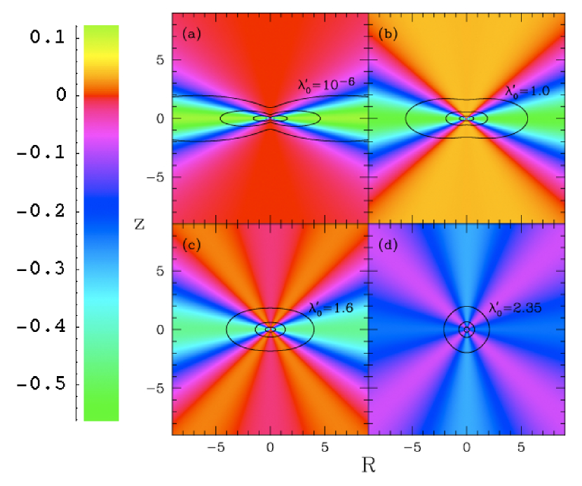
Figure 5: Two-dimensional isodensity contours (black lines) and mass flux contours (per unit solid angle; colors) for four of the solutions shown in Fig. 2 with $\alpha=0.1$, $\epsilon^{\prime}=10$ and $\lambda_{0}^{\prime}=10^{-6}$ (a), 1.0 (b), 1.6 (c), and 2.35 (d). The net inflow rate is normalized to $\dot{m}=1$ in all cases. The axes are labeled in terms of cylindrical coordinates $R$ and $z$.

Figure 5 illustrates in a different way the flow geometry and the relative importance of the rates of mass inflow and outflow, for four of the solutions shown in Fig. 2 ($\alpha=0.1$, $\epsilon^{\prime}=10$). Isodensity contours are shown by solid lines, while color contours trace the flux of mass per unit solid angle ($=\rho v_{r}$). The scale of the cylindrical coordinates ($Rz$) used to label the axes, as well as the isodensity contour levels, are arbitrary because of the radially self-similar nature of the solutions considered.

Figure 6 summarizes the most significant results for the existence and the properties of outflows that emerged from our systematic survey of the parameter space of hot accretion flow solutions with conduction. Focusing on the specific $\alpha=0.1$ case, the various curves in Fig. 6 cover the $(\epsilon^{\prime},\lambda_{0}^{\prime})$ space. The four panels show (a) the flow radial velocity at the pole, $v_{r}(\theta=0)$, in units of the Keplerian value, (b) the angular velocity at the equator, $\Omega(\theta=\pi/2)$, in units of the Keplerian value, (c) the opening angle of outflowing regions, including conical outflow cases, and (d) the ratio of outflowing to net inflowing mass rate (which is also the accretion rate defined in Eq. [27]).

A number of clear trends emerge from this parameter space survey. Solutions with small $\epsilon^{\prime}$ values ($\mathrel{\hbox to0.0pt{\lower 3.0pt\hbox{$\mathchar 536\relax$}\hss}\raise 2.0pt\hbox{$\mathchar 316\relax$}}1$) do not exhibit outflows, but only pure inflow regimes. Conversely, solutions with the largest values of $\epsilon^{\prime}$ are the most efficient at producing outflows. Furthermore, even among the solutions with $\epsilon^{\prime}\mathrel{\hbox to0.0pt{\lower 3.0pt\hbox{$\mathchar 536\relax$}\hss}\raise 2.0pt\hbox{$\mathchar 318\relax$}}1$, there is only a finite range of $\lambda_{0}^{\prime}$ values for which an outflow regime exists. The larger $\epsilon^{\prime}$ is, the larger are the velocity, opening angle and mass flux of the outflow, and so is the maximum value of $\lambda_{0}^{\prime}/\epsilon^{\prime}$ beyond which the outflow ceases to exist. We also find that solutions with conical outflows exist only for sufficiently high $\epsilon^{\prime}$ values. Finally, for large $\epsilon^{\prime}$ solutions, the outflowing regime persists even to very small values of $\lambda_{0}^{\prime}/\epsilon^{\prime}$ but outflows become increasingly weaker, slower and narrower. It should not be a surprise that these various flow properties scale with the ratio $\lambda_{0}^{\prime}/\epsilon^{\prime}$, given the form of the energy equation (Eq. [23]). All these trends are consistent with the detailed results shown in Figs. 2 and 3.

The increased efficiency of large $\epsilon^{\prime}$ solutions at producing outflows can be interpreted as resulting from the larger latitudinal temperature gradients present in these solutions. This makes the contribution of the polar conduction term more important, relative to the radial conduction term (which is tied to a fixed radial temperature gradient set by self-similarity). Mass outflow rates $\sim 6\%$ of the net inflow rate, outflow velocities $\mathrel{\hbox to0.0pt{\lower 3.0pt\hbox{$\mathchar 536\relax$}\hss}\raise 2.0pt\hbox{$\mathchar 316\relax$}}2\%$ of the local Keplerian velocity and outflow opening angles $\sim 50$ degs are reached in solutions with $\epsilon^{\prime}=10$ and $\lambda_{0}^{\prime}\simeq 0.1$. For even larger values of $\epsilon^{\prime}$, outflow properties continue to follow the trends shown in Fig. 6. For instance, we have found $\epsilon^{\prime}=50$ solutions with mass outflow rates $\mathrel{\hbox to0.0pt{\lower 3.0pt\hbox{$\mathchar 536\relax$}\hss}\raise 2.0pt\hbox{$\mathchar 316\relax$}}13\%$ of the net inflow rate, outflow velocities $\mathrel{\hbox to0.0pt{\lower 3.0pt\hbox{$\mathchar 536\relax$}\hss}\raise 2.0pt\hbox{$\mathchar 316\relax$}}3\%$ of the local Keplerian velocity and outflow opening angles $\mathrel{\hbox to0.0pt{\lower 3.0pt\hbox{$\mathchar 536\relax$}\hss}\raise 2.0pt\hbox{$\mathchar 316\relax$}}60$ degs. Numerical convergence becomes increasingly difficult at large $\epsilon^{\prime}$ values, however, and we have not explored this regime as systematically as the low $\epsilon^{\prime}$ one.

Two additional features in Fig. 6 are worth emphasizing. All solutions reach the non-rotating limit for values of $\lambda_{0}^{\prime}/\epsilon^{\prime}\approx 0.24$ and $v_{r}\mathrel{\hbox to0.0pt{\lower 3.0pt\hbox{$\mathchar 536\relax$}\hss}\raise 2.0pt\hbox{$\mathchar 316\relax$}}-0.06~{}v_{\mathrm{K}}$. A derivation of these asymptotic values for the non-rotating limit is provided in Appendix B. We also find that there is a wedge in the $\lambda_{0}^{\prime}/\epsilon^{\prime}$ vs. $\epsilon^{\prime}$ space, such that solutions do not exist for a growing range of $\lambda_{0}^{\prime}/\epsilon^{\prime}$ as the value of $\epsilon^{\prime}$ is increased. Despite careful efforts to reach numerical convergence in these parts of the parameter space, we have failed to find solutions of sufficient numerical accuracy (or at all) in these regions. We have not clearly identified the origin of this difficulty. Let us stress that all the solutions shown in figures, and otherwise discussed in this work, have reached satisfactory numerical convergence.

We find that the value of the viscosity parameter, $\alpha$, affects quantitatively (but not qualitatively) the properties of hot accretion flow solutions with conduction. For larger values of $\alpha$, the radial inflow and outflow speeds are increased and the overall density scale is reduced, as expected from the original ADAF $\alpha$ scalings. Figure 4 shows a specific comparison of solutions with $\epsilon^{\prime}=10$, $\lambda_{0}^{\prime}/\epsilon^{\prime}=0.1$ and $\alpha=0.02$, $0.1$ and $0.2$. The outflow speed is much larger in the $\alpha=0.2$ solution, reaching a value $\simeq 0.11\,v_{\rm K}$ at the pole. Yet, the mass outflow rate ($\sim 9\%\,\dot{m}$) is not much greater in the $\alpha=0.2$ solution than in the other two solutions ($\sim 6$-$7\%\,\dot{m}$) because of the reduced density scale associated with faster radial velocities. The outflow opening angles are comparable in all three solutions. For consistency and conciseness, we focus on solutions with $\alpha=0.1$ below.

4.2.2 Detailed Energy and Momentum Balance

To understand better the various properties of these hot accretion flows with conduction, let us now focus on the detailed energy and momentum balance that they satisfy.

Figure 7 shows latitudinal profiles of the advection term (a), on the LHS of the energy equation (Eq. [23]), and of the conduction (b) and viscous (c) terms, on the RHS of Eq. (23), for the same specific sequence of solutions as shown in Fig. 2 ($\alpha=0.1$, $\epsilon^{\prime}=10$). In the solution with negligibly small conduction ($\lambda_{0}^{\prime}=10^{-6}$), the advection and the viscous terms balance each other exactly and heat advection acts to cool the flow (which corresponds to positive values in panel a). In the solution with $\lambda_{0}^{\prime}=1.0$, however, the magnitude of the conduction term is already very important, being comparable to or larger than the magnitude of the viscous term in most of the flow. In addition, conduction both cools the flow in the polar regions (which corresponds to negative values in panel b) and heats it up in the equatorial regions. As a result of this cooling of the polar regions (where the contribution from the viscous term is comparatively small, simply by geometry), the balance between these various terms permits a negative advection term in the polar regions, which corresponds to advective heating and outflow.

As the value of $\lambda_{0}^{\prime}$ reaches $1.6$, the latitudinal profile of temperature starts to flatten significantly (see Fig. 2), thus reducing the contribution of the polar component of conduction. The radial component, on the other hand, is strictly positive and can only increase in magnitude with the value of $\lambda_{0}^{\prime}$ (because of the radial self-similarity of the solutions). As a result, the net conduction term switches sign again in the polar regions (which are now heated by conduction), but it is able to remain somewhat negative at intermediate values of the polar angle, $\theta$. This situation leads to the conical outflow regime previously identified.

Finally, for even larger values of $\lambda_{0}^{\prime}(\geq 2)$, the radial component of conduction dominates everywhere over the polar component (which is further reduced by the continued flattening of the temperature profile; Fig. 2), thus forcing the net conduction term to act strictly as a heat source (as in the 1D solutions of §3). The energy equation is then satisfied only if advection acts to cool the flow everywhere, which must then be globally inflowing. For the largest values of $\lambda_{0}^{\prime}$ considered, advection very nearly balances conduction as the viscous term drops precipitously and the non-rotating limit is reached. In good analogy with what we have seen for 1D solutions with conduction in §3, the non-rotating Bondi-like limit corresponds to strict equality between conduction and advection.

From this examination of energy balance in our radially self-similar solutions, it is clear that the key to thermal outflows is the existence of strong enough cooling in the flow for advection to be allowed to act as a heat source. This is preferentially achieved in polar regions, simply because these are regions where the rate of viscous dissipation must drop by geometrical constraint.

Let us comment here on the fact that the advection parameter, $f$, is actually ill-defined in our solutions with conduction. Since $f$ is associated with the viscous dissipation term in Eq. (23), it represents a form of cooling which is proportional to the rate of viscous dissipation. As a result, in solutions with an energy balance dominated by conduction (e.g. solutions with large $\lambda_{0}^{\prime}$ in Fig. 7), a small value of $f$ ($\ll 1$) does not correspond to a globally efficient cooling anymore, as it used to in the original ADAF solutions. This undesirable situation would disappear in 2-temperature solutions with more realistic descriptions of cooling, such as the ones described by Narayan & Yi (1995b). Note also that this is not a critical flaw for our analysis: the energetics of all the solutions discussed here depends only on the value of $\epsilon^{\prime}\equiv\epsilon/f$, so that large $\epsilon^{\prime}$ values can equally well be interpreted as corresponding to low $\gamma$ values.

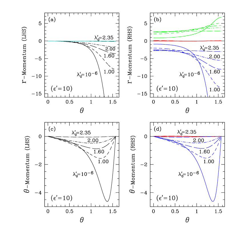
Figure 8: Latitudinal profiles of terms in the $r$- and $\theta$-components of the momentum balance equation in five solutions with $\alpha=0.1$, $\epsilon^{\prime}=10$ and varying degrees of conduction (as measured by $\lambda_{0}^{\prime}$). Top panels: left- and right-hand sides of the radial momentum equation (Eq. [20]). (a) shows the magnitude of the inertial term (cyan) and the centrifugal term (black) on the LHS of the $r$-momentum equation. (b) shows contributions to the RHS of this same equation: gravitational (blue), pressure gradient (green) and viscous (red) terms. Bottom panels: left- and right-hand sides of the latitudinal momentum equation (Eq. [21]). (c) shows the magnitude of the centrifugal term (black). (d) shows contributions from the pressure gradient (blue) and viscous (red) terms.

For completeness, we now examine in detail the momentum balance in these same solutions ($\alpha=0.1$, $\epsilon^{\prime}=10$). Figure 8 shows latitudinal profiles of various terms in the radial and polar components of the momentum equation (Eqs. [20] and [21], respectively). The magnitude of the various terms on the LHS and the RHS of these equations are labeled with different colors in the panels of Fig. 8, for the same sequence of increasing $\lambda_{0}^{\prime}$ values as before. Note that we ignore the azimuthal momentum equation, which simply expresses angular momentum conservation.

For a negligibly small level of conduction ($\lambda_{0}^{\prime}=10^{-6}$), the $r$-momentum balance is dominated by pressure support against gravity in the polar regions, while rotational support becomes gradually dominant in the equatorial regions. As the value of $\lambda_{0}^{\prime}$ is increased, the flow becomes hotter, more spherically symmetric and the $r$-momentum balance tends to be more dominated by pressure support at all values of the polar angle, $\theta$. The inertial and viscous terms are never very important for $r$-momentum balance along this $\lambda_{0}^{\prime}$ sequence. As for the $\theta$-momentum equation, for all values of $\lambda_{0}^{\prime}$ considered, it is satisfied through a balance between latitudinal pressure gradients and projected centrifugal force, with little contribution from the viscous terms. Perhaps one of the most interesting property of the profiles shown in Fig. 8 is that they show explicitly that there is no distinction, from the point of view of momentum balance, between inflowing and outflowing regions of the flow. This confirms that outflows, when they exist, are purely determined by energetic considerations. This further justifies us classifying them as “thermal” in origin.

4.2.3 The Bernoulli Parameter

Much of the discussion in the literature on the likelihood of outflows from hot accretion flows is articulated around the value of the Bernoulli parameter, $B_{\rm e}$ (or, more generally, the Bernoulli function). Narayan & Yi (1994; 1995a) first emphasized the positivity of $B_{\rm e}$ in their solutions and raised the possibility that this would lead to bipolar outflows. Furthermore, Blandford & Begelman (1999)’s motivation and method to develop ADIOS is rooted in the notion that hot accretion flows with positive $B_{\rm e}$ must have outflows and that their structure and properties should be accordingly modified, leading to a mass accretion rate varying with radius. The relevance of the value of $B_{\rm e}$ for the generation of outflows has also been discussed in the context of numerical simulations (e.g. Stone et al. 1999) and it has been put into question (e.g. Abramowicz et al. 2000). Since our hot accretion flow solutions with conduction produce outflows spontaneously, it is of considerable interest to study the relation between these outflows and the value of $B_{\rm e}$ in the solutions.

Figure 9 shows latitudinal profiles of the dimensionless Bernoulli parameter, $b(\theta)=B_{\rm e}/(r\Omega_{\rm K})^{2}$ (same notation as Narayan & Yi 1995a) in a set of solutions with $\alpha=0.1$, $\gamma=1.5$ and different values of $f$ and $\lambda_{0}^{\prime}/\epsilon^{\prime}$. In addition to $b(\theta)$, scaled latitudinal profiles of the radial velocity, $v_{r}$, are shown, for an easy identification of inflowing vs. outflowing regions. The nine panels in Fig. 9 are organized in such a way that the three rows correspond to $\epsilon^{\prime}\simeq 10$, $2$ and $0.5$, from top to bottom, with increasing values of $\lambda_{0}^{\prime}/\epsilon^{\prime}$ from left to right.

From this ensemble of solutions, one concludes that the positivity of $b(\theta)$ does not in general discriminate between inflowing and outflowing regions in our solutions. Although the solution corresponding to $f=0.033$ and $\lambda_{0}^{\prime}/\epsilon^{\prime}=0.1$ would seem to indicate it does, this is in fact a coincidence since we find many counterexamples. Notice in particular in Fig. 9 how solutions with $b(\theta)$ changing from positive at the pole to negative at the equator can be alternatively (nearly) static, outflowing or inflowing at the pole. Similarly, solutions with globally positive values of $b(\theta)$ can be globally inflowing without any difficulty.

The additional panels in Figure 10 show two particularly striking examples of the loose relation between the sign of $b(\theta)$ and the inflow/outflow properties of our solutions. In one solution, with $\lambda_{0}^{\prime}/\epsilon^{\prime}=0.16$, the outflow has a conical geometry. While the value of $b(\theta)$ decreases monotically with $\theta$, the radial velocity is clearly not monotonic, with two sign changes. In the other solution, with $\lambda_{0}^{\prime}/\epsilon^{\prime}=0.02$, the outflow is polar but there is a small regions at mid-latitudes where outflowing gas has negative $b(\theta)$ value. Although this type of “violation” is generally marginal, it clearly demonstrates that there is no strict relation between the sign of $b(\theta)$ and the inflow/outflow properties of gas in our solutions. It should be noted that for large enough values of $\lambda_{0}^{\prime}$, one would expect the Bernoulli parameter (which is an adiabatic, inviscid quantity) to lose its physical significance, since the flow must then become strongly diabatic. We suspect that the $b(\theta)<0$ outflow region shown in the left panel of Fig. 10 and the globally inflowing solutions with globally positive $b(\theta)$ values shown in Fig. 9 are all manifestations of this loss of significance of $b(\theta)$ in flows with significant conduction.

5 Relevance to Observational Trends

It is difficult to evaluate, from self-similar solutions alone, what the radiative efficiency of hot accretion flows with conduction may be. In our solutions, the flow structure adjusts so that the divergence of the conduction flux generated in the innermost regions is balanced by an increased level of entropy advection. There will be no extra source of energy available in the presence of conduction (in fact less is available in our solutions, since the viscous dissipation rate drops with $\Omega$), but the dissipated energy is redistributed differently in flows with conduction than in flows without. This redistribution affects the local flow properties (density, temperature), which in turn affect its cooling properties.

Using our 1D solution scalings (§3) for simplicity, it is possible to estimate crudely the modified level of emission expected relative to a standard ADAF. Free-free emission scales as $\rho^{2}T^{1/2}\propto(c_{s0}v_{0}^{2})^{-1}$ for a given value of the accretion rate, $\dot{M}$. We find that this emission is effectively reduced, e.g. by as much as $\sim 25\%$ in the 1D solution of Fig. 1 with $\gamma=1.5$ (and much more in the $\gamma=1.1$ solution). Even though conduction heats up the gas locally, the reduced density resulting from the larger inflow speed dominates, leading to a net decrease in the expected level of free-free emission. On the other hand, the very steep dependence of synchrotron emission on the electron temperature (e.g. Mahadevan 1997) suggests that hotter solutions (with conduction) may be radiatively more efficient from the point of view of that process. These are only rough scalings, however. In light of several complications expected in global solutions with conduction (see discussion in §6), it is unlikely that we can determine, from self-similar solutions alone, how the global radiative efficiency of a hot accretion flow may be affected by conduction. We postpone a thorough discussion of this important issue to future work and focus here instead on the possible relevance of the outflows found in our solutions to a variety of observationally established trends for accreting black holes.

In recent years, much progress has been made in understanding the outflow/jet properties of accretion flows around black holes in X-ray binaries and Active Galactic Nuclei. Various observational studies suggest that, in both classes of systems, there is a regime of steady outflow when black holes accrete well below the Eddington rate (for luminosities $\mathrel{\hbox to0.0pt{\lower 3.0pt\hbox{$\mathchar 536\relax$}\hss}\raise 2.0pt\hbox{$\mathchar 316\relax$}}0.01-0.1L_{\rm Edd}$), while the outflow regime becomes flaring/unsteady at higher accretion rates (e.g. Ho 2002; Gallo, Fender, Pooley 2003; Merloni, Heinz & Di Matteo 2003; Fender, Belloni & Gallo 2004; Nipoti, Blundel & Binney 2005; Sikora, Stawarz & Lasota 2006). Some of the latest results support the notion that black holes accreting at sub-Eddington rates do so through an advective form of accretion (e.g. Greene, Ho & Ulvestad 2005; Koerding, Fender & Migliari 2006), but there is some evidence in the “low/hard” state of at least two Galactic black hole systems (Miller et al. 2006) that a standard thin disk remains embedded in the hot flow (a situation which may favor outflows according to our large $\epsilon^{\prime}$ solutions). It is tempting to relate these various observational trends with our results on thermal outflows from steady, hot accretion flows with conduction.

The association would be strengthened if one could show that thermal conduction is expected to be equally important in hot accretion flows around stellar-mass and supermassive black holes. After all, we made the case for weakly-collisional accretion conditions only for systems harboring supermassive black holes in §2. While the temperature profile does not depend on black hole mass in self-similar solutions scaled in units of the Schwarzschild radius, density profiles do. To address this question, we compare the scalings for the coefficient of turbulent viscosity ($\nu=\alpha c_{s}^{2}/\Omega_{\rm K}$) and the Spitzer coefficient of thermal diffusivity ($\chi\propto T^{5/2}/\rho$), using for simplicity the ADAF scalings in Schwarzschild units of Narayan et al. (1998b). The comparison of these two diffusivity coefficients is the relevant one since it captures the relative magnitude of “viscous” and conduction effects on any scale of interest. We find that the two coefficients scale identically (linearly) with the mass of the central black hole, which suggests that conduction would indeed be equally important in hot accretion flows around stellar-mass and supermassive black holes. This conclusion is also consistent with the similar scalings with black hole mass of the accretion time and collision times discussed by Mahadevan & Quataert (1997). It would be interesting to strengthen this comparison by using, as much as possible, observational constraints on hot accretion flows in X-ray binaries, as we have done for AGN in §2.

Establishing on a firmer ground the relevance of the thermal outflows found in our solutions to observational trends for accreting black holes will clearly require additional work. In the meantime, we note that our solutions allow a direct scaling of the expected outflow power, per unit accreted mass, which is a quantity of obvious interest. Recalling that the Bernoulli constant, $b(\theta)$, represents the asymptotic value of the energy of gas escaping from the central mass gravity, we can use it as a measure of the outflowing energy rate and compare that to the rate of energy release due to accretion. The outflow power is simply $P_{\rm out}=\dot{M}_{\rm out}b(\theta)v_{\rm K}^{2}$. The accretion power is $P_{\rm acc}\simeq 0.1\dot{M}_{\rm in}c^{2}$ , if we pick a radius of maximum energy release of $\sim 3$ Schwarzschild radii to fix the accretion efficiency to $\sim 0.1$ as is usually done. At $3R_{\rm s}$, $v_{\rm K}^{2}\sim c^{2}/6$. For a ratio of $\dot{M}_{\rm out}/\dot{M}_{\rm in}\sim 0.05$ (solutions with $\epsilon^{\prime}=10$ in Fig. 6) and a corresponding value of $b(\theta)\sim 0.15$ for outflowing regions (Fig. 9), we deduce a ratio $P_{\rm out}/P_{\rm acc}$ that reaches up to $\sim 1\%$ in our solutions. Therefore, provided that solutions with realistic cooling properties can be constructed with radiative efficiencies $<10^{-3}$ (i.e. less than a hundredth of the fiducial $0.1$ value), it may be possible to explain the “jet-power dominance” of radiatively-inefficient accretion flows which has been recently emphasized by several authors (e.g. Nagar, Falcke & Wilson 2005; Koerding et al. 2006; Allen et al. 2006). Interestingly, values of $P_{\rm out}/P_{\rm acc}\mathrel{\hbox to0.0pt{\lower 3.0pt\hbox{$\mathchar 536\relax$}\hss}\raise 2.0pt\hbox{$\mathchar 316\relax$}}1\%$ as we just derived are comparable to the values of $P_{\rm jet}/P_{\rm Bondi}$ of a few percents inferred by Allen et al. (2006).

In this context, understanding how thermal outflows may relate to the relativistic jets of accreting black holes will likely be important. After all, outflow velocities decrease with radius as $r^{-1/2}$ in our solutions (by virtue of self-similarity), which is a rather unappealing feature. Thermal outflows could be collimated and accelerated by their environment or, alternatively, they could contribute to the collimation and acceleration of narrower and faster jets, such as the ones emerging in relativistic MHD numerical simulations of adiabatic tori (e.g. DeVilliers et al. 2005; Hawley & Krolik 2006).

One of the best systems available to us for the study of radiatively-inefficient accretion flows (and related outflows) is Sgr A*. In recent years, the focus of theoretical work to interpret the rich set of data has in fact shifted to include a jet or outflow component (e.g. Falcke & Biermann 1999; Falcke & Markoff 2000; Melia & Falcke 2001; Markoff et al. 2001; Yuan, Markoff & Falcke 2002). Observations of the size (e.g. Bower et al. 2004; Shen et al. 2005; Yuan, Shen, Huang 2006), variability (e.g. Yuan, Quataert & Narayan 2003; Yusef-Zadeh et al. 2006) and polarization (e.g. Agol 2000; Quataert & Gruzinov 2000b; Bower et al. 2003; Marrone et al. 2006) of this source all have tremendous potential to further constrain the properties of the hot accretion flow and its outflow, and they may be able to help us discriminate between the thermal outflows seen in our solutions and other outflow alternatives. Direct constraints on outflow geometries for accreting black holes are generally scarce, but it is interesting to note that Junor, Biretta & Livio (1999) observe an opening angle $\sim 60$ degs at the base of the radio jet in M87, in line with the wide outflow geometries found in our solutions. On the other hand, other geometries have been proposed for other classes of systems (e.g. Elvis 2000).

The motivation to understand the nature and properties of outflows from accreting black holes goes beyond what we have just outlined, as outflows may be an efficient process by which black holes influence their environments. Recently, this general point has been raised in the specific context of radiatively-inefficient accretion flows by several groups. Soria et al. (2006a,b; see also Di Matteo, Carilli & Fabian 2001) invoked slow outflows to effect a feedback on the rate of Bondi accretion in several low-luminosity AGN. The wide outflow geometries in our solutions may suggest that the conceptual use of a simple Bondi spherical inflow geometry to estimate gas capture rates is inappropriate if indeed a large fraction of the black hole capture sphere is the site of gas outflow. The work of Nagar et al. (2005) and Allen et al. (2006) further suggests that feedback due to outflows associated with radiatively-inefficient accretion flows can reach far beyond the black hole immediate vicinity and affect star formation in the host galaxy, or even the surrounding hot gas when the host is located at the center of a group or a cluster of galaxies. It will be interesting to develop these arguments, and more detailed feedback scenarios (e.g. Vernaleo & Reynolds 2006), in light of what we have learned in our study of thermal outflows.

6 Discussion and Conclusion

The possibility that tangled magnetic fields strongly limit the efficiency of thermal conduction in a hot flow constitutes a major theoretical uncertainty for our models. In recent years, a similar issue has been discussed in the context of galaxy cluster cooling flows. Several studies have concluded that magnetic fields may not limit too strongly the efficiency of thermal conduction (e.g. Narayan & Medvedev 2001; Gruzinov 2002; see also Chandran & Cowley 1998; Chandran et al. 1999), but this remains somewhat of an open issue. If tangled magnetic fields were to limit the effective mean free paths in the hot flow to $l_{\rm eff}\mathrel{\hbox to0.0pt{\lower 3.0pt\hbox{$\mathchar 536\relax$}\hss}\raise 2.0pt\hbox{$\mathchar 316\relax$}}R$, conduction would likely still have important consequences for the flow structure and properties. If, on the other hand, tangled magnetic fields act to make $l_{\rm eff}\ll R$, a much weaker role for conduction (if any) is to be expected. Explicit numerical simulations with anisotropic conduction along field lines in an MHD turbulent medium could greatly help in settling this issue (see, e.g., Cho & Lazarian 2004; Sharma et al. 2006). It should be emphasized that the energy transport mechanism which permits the existence of outflows in our solutions does not have to be thermal conduction. Any form of heat transport (e.g. turbulent, as emphasized by Balbus 2004) acting like thermal conduction would have similar consequences for the flow.

One of several limitations of our self-similar hot accretion flow solutions with conduction is their 1-temperature structure. Narayan & Yi (1995b) have shown how crucial it is to account for the 2-temperature structure of the hot flow to obtain solutions with realistic cooling properties. In such solutions, the expected decoupling of electron and ion temperatures in the inner regions of the hot flow would modify the role of conduction. For one thing, ions may be partially insulated from electron conduction. In addition, self-similarity is broken in the 2-temperature regime and the electron temperature profile flattens to a sub-virial slope (e.g. Narayan et al. 1998b). In global solutions, conduction is expected to flatten both the polar and the radial temperature profiles (while it only affects the polar profile in the radially self-similar solutions discussed here). Furthermore, if a saturated form of conduction is appropriate, the saturated flux should be reduced in regions of the flow where the electrons become relativistic, since their “free streaming” velocity then becomes limited by the speed of light. Finally, the break-down of self-similarity implies that the radial contribution to conduction, which acts only to heat up the flow in our solutions, will have to be done at the expense of inner regions that will now be cooling by conduction. Clearly, it will be interesting to see how all these effects combine with each other in global models of hot accretion flows with conduction.

A potentially more fundamental limitation of our work may be the use of simple fluid equations to describe a weakly-collisional plasma obeying a more complex set of equations. For instance, Balbus (2001) has argued that the dynamical structure of hot flows could be affected by the anisotropic character of conduction in the presence of magnetic fields (see also Parrish & Stone 2005), while Quataert et al. (2002) have emphasized additional effects due to the anisotropic pressure tensor present in the weakly-collisional regime (see also Sharma et al. 2006). On the other hand, it is possible that a scale analysis could justify the use of simpler fluid equations to describe the dynamics of the weakly-collisional magnetized plasma on the largest scales of interest in the context of hot accretion flows. Such an analysis would clearly be valuable since essentially all the literature on hot accretion flows relies on collisional fluid equations (magnetized or not).

In recent years, much emphasis has been put on reducing the rate at which gas is accreted by a central black hole, within a hot flow, either by arguing that a negative Bernoulli constant is required for an accretion solution with imposed winds to be physically viable (Blandford & Begelman 1999) or by invoking a gradual reduction in the rate of mass accretion in the flow due to the effects of convection (Narayan et al. 2000; Quataert & Gruzinov 2000a). Our results, combined with the possibility that conduction may be important in hot accretion flows, could pose a challenge to both of these scenarios. We have already seen that the sign of the Bernoulli constant does not determine the existence of thermal outflows, or even discriminate between inflowing and outflowing regions, in our solutions with conduction. Our solutions also show that a radially varying $\dot{m}$ is not necessarily associated with the existence of such outflows. In addition, if conduction is important on all scales of interest in the hot flow, convection may be suppressed altogether when a displaced fluid element efficiently reaches thermal equilibrium with its environment through conduction.

Obviously, our results do not exclude the existence of other classes of spontaneously outflowing solutions with radially varying $\dot{m}$, density profiles deviating from the canonical $r^{-3/2}$, more realistic flow patterns allowing for non-zero latitudinal velocities, polar funnels, or a role for other radial and latitudinal energy/momentum transport mechanisms (see, e.g., the issues of adiabatic stability discussed in Blandford & Begelman 2004, but also Balbus 2001 for the diabatic case with anisotropic conduction and magnetic fields). It would be particularly interesting to contrast the study of these generalized solutions with the results for averaged flow properties emerging from simple hydrodynamical and MHD numerical simulations (e.g. McKinney & Gammie 2002; Proga 2005), in an effort to make the best use of these two complementarity approaches to the black hole accretion problem.

If conduction is generally important in hot accretion flows around black holes, it could have additional interesting consequences besides the ones illustrated in our specific solutions. For instance, if the hot flow residing inside the capture radius around a black hole is able to heat up the ambient gas outside of that capture radius, the Bondi rate of gas capture ($\propto c_{s}^{-3}$) may be effectively reduced. While Gruzinov (1998) invoked “turbulent” heat flows to achieve this, the weakly-collisional conditions discussed in §2 for several galactic nuclei suggest that this could be done by “microscopic” conduction itself. More detailed models are therefore needed to address various interesting issues related to conduction, to understand better how conduction may affect the structure and properties of hot accretion flows and to determine how these effects may relate to the observational characteristics of dim accreting black holes.

Appendix A Prescriptions for Conduction

In §3, we have seen that a saturated form of conduction scales in such a way that it permits 1D radially self-similar solutions. Consequently, we first attempted to find 2D radially self-similar solutions with a saturated conduction flux written as

$${\bf F_{{\rm s}}}=\,-5\Phi_{{\rm s}}\rho c_{s}^{3}\frac{{\bf\nabla}T}{|{\bf\nabla}T|},$$ (A1)

which depends only on the direction of the local temperature gradient, not its magnitude. From taking minus the divergence, we obtained the following conduction term in the energy equation:

$$Q_{{\rm s}}(\theta) = 5\Phi_{{\rm s}}\Big{\{}\frac{P(\theta)c_{s}(\theta)}{\sqrt{1+\left(\frac{d}{d\theta}\log c_{s}^{2}(\theta)\right)^{2}}}$$

$$+\frac{1}{\sin\theta}\frac{d}{d\theta}\left[\sin\theta\frac{P(\theta)c_{s}(\theta)}{\sqrt{1+\left(\frac{d}{d\theta}\log c_{s}^{2}(\theta)\right)^{2}}}\frac{d}{d\theta}\log c_{s}^{2}(\theta)\right]\Big{\}},$$ (A2)

within the framework of our self-similar solutions.

We have found this prescription to be numerically unstable, or at least difficult to work with. This may be due to the explicit coupling between the radial and polar conduction terms that appears within this prescription (which does not seem well suited to our separable, radially self-similar solutions). It may also be caused by the structure of the mathematical operator resulting from this prescription: it no longer acts as a diffusion process.

Consequently, in our 2D treatment (in §4), we returned to a standard diffusive operator for conduction, with a conductivity coefficient scaled with radius to preserve self-similarity. This results in the following conduction term in the energy equation (see also Eq. [23]):

$$Q_{{\rm d}}(\theta)=\,\lambda_{0}\left[c_{s}^{2}(\theta)+\frac{1}{\sin\theta}\frac{d}{d\theta}\left(\sin\theta\frac{dc_{s}^{2}(\theta)}{d\theta}\right)\right].$$ (A3)

From a comparison of these two prescriptions, it is clear that, in the limit of strong conduction, when latitudinal profiles of most flow quantities become nearly flat, the two conduction parameters, $\Phi_{\rm s}$ and $\lambda_{0}$, are simply related to each by $\lambda_{0}\approx\,5\rho(\theta)c_{s}(\theta)\,\Phi_{{\rm s}}$. Using the simple scalings of Appendix B, the relation becomes

$$\lambda_{0}\approx\,\frac{5\sqrt{10}}{6\pi}\frac{\dot{m}}{\alpha}\,\Phi_{{\rm s}}=8.4\,\Phi_{{\rm s}},$$ (A4)

where we have used $\dot{m}=1$, $\alpha=0.1$ for the last equality. This correspondence is helpful in showing that, in all our 2D solutions, the non-rotating limit is reached for $\Phi_{{\rm s}}$ equivalent values which are $\ll 1$, in good agreement with our 1D results (in §3). In other words, even in 2D solutions, a level of conduction well below that of the (non-relativistic) saturated conduction flux is sufficient to alter the structure and properties of hot accretion flows substantially.

Appendix B Maximum Value of the Conduction Coefficient

As we have seen in §4, for a given value of the flow parameter $\epsilon^{\prime}$, there is a maximum value of the conduction parameter, $\lambda_{0}^{\prime}$, at which the solutions reach the non-rotating, Bondi-like limit. No solutions of physical significance exist beyond this maximum value since they would require imaginary values of $\Omega$, as we shall now establish. Let us evaluate Eqs. (20–23), at the flow equator, using adequate boundary conditions, in the limit of low viscosity ($\alpha v\ll 1$), small radial velocity ($v^{2}\ll 1$) and under the assumption that second order derivatives with respect to $\theta$ become small (which is generally accurate for solutions approaching the non-rotating limit). We obtain:

$$\frac{2}{5}(1-\Omega^{2}), \approx c_{s}^{2}$$ (B1)

$$(\frac{v_{r}}{c_{s}^{2}}+\frac{3}{2}\alpha)\Omega \approx 0,$$ (B2)

$$-\frac{3}{2}\epsilon^{\prime}v_{r}-\frac{\lambda_{0}^{\prime}}{\rho} \approx \frac{9}{4}\alpha\Omega^{2}.$$ (B3)

The first equation establishes that, in the strong conduction limit, $c_{s}^{2}\approx\frac{2}{5}$. The second equation yields, in combination with the first, $v_{r}\sim-\frac{3}{5}\alpha$, in the same limit. To be exact, this is not the limit $\Omega\approx 0$, but rather $d^{2}\Omega/d\theta^{2}\approx 0$. The actual non-rotating limit occurs at a slightly lower value of $v_{r}\mathrel{\hbox to0.0pt{\lower 3.0pt\hbox{$\mathchar 536\relax$}\hss}\raise 2.0pt\hbox{$\mathchar 316\relax$}}-\frac{3}{5}\alpha$. The third equation places the explicit constraint on $\lambda_{0}^{\prime}$ for the non-rotating limit, since the left-hand side must be positive for the value of $\Omega$ to be real. This fixes the maximum value of the conduction parameter $\lambda_{0}$ to

$$\lambda_{0,{}\max}(\dot{m},\epsilon)\approx\frac{3}{4\pi}\dot{m}\epsilon=0.24\dot{m}\epsilon,$$ (B4)

where we have used the crude approximation that momentum ($\rho v_{r}$) profiles are uniform along $\theta$, which results in $\rho(\theta)\sim 5\dot{m}/(6\pi\alpha)$. This estimate of the maximum value of $\lambda_{0}$ agrees well with our numerical results (e.g. in Fig. 6).

Appendix C Comparison with Anderson (1987)

Our results on 2D hot accretion flows with conduction share strong similarities with those of Anderson (1987). First, let us mention that we have succeeded in reproducing many of the results reported by this author, using the same prescription for conduction ( i.e. with a conduction coefficient which scales not only with radius, but also with the local flow viscosity and density). With this prescription, the conduction term in the energy equation becomes:

$$Q_{{\rm A}}=\,\alpha\lambda_{1}\left[P(\theta)c_{s}^{2}(\theta)+\frac{1}{\sin\theta}\frac{d}{d\theta}\left(\sin\theta P(\theta)\frac{dc_{s}^{2}(\theta)}{d\theta}\right)\right].$$ (C1)

Returning to our analysis, there are still differences between our work and that of Anderson (1987), both in the formalism and in the results. Anderson works in the limit of “weak shear viscosity,” with several viscous terms dropped from the dynamical equations (as compared to ours). He adopts a polytropic equation of state, a prescription for viscosity which differs from Shakura-Sunyaev and there is no inertial term in his radial momentum equation. As a result, his set of differential equations is reduced to a third order system, as opposed to a seventh order one in our case. Despite these technical differences, our results are qualitatively consistent with many of his conclusions. Differences appear mostly at the quantitative level, for instance in the rates of mass outflow (which appear a few times larger in our solutions). One qualitative feature which has apparently been missed by Anderson (1987) is the existence of solutions with conical outflow geometries in sub-regions of the parameter space.

From this comparison, we can safely conclude that many of the qualitative features exhibited by our solutions should be relatively robust to changes in the various prescriptions adopted (e.g. conduction and viscosity).

Nucleus	$n_{1^{\prime\prime}}$	$T_{1^{\prime\prime}}$	$R_{1}$	$l_{1}/R_{1}$	$l_{1}/R_{\rm cap}$
	(cm-3)	($10^{7}$ K)	(cm)
Sgr A*	$100$	$2.3$	$1.3\times 10^{17}$	$0.4$	$0.4$
NGC 1399	$0.3$	$0.9$	$3.1\times 10^{20}$	$0.009$	$0.02$
NGC 4472	$0.2$	$0.9$	$2.5\times 10^{20}$	$0.016$	$0.07$
NGC 4636	$0.07$	$0.7$	$2.2\times 10^{20}$	$0.032$	$0.6$
M87	$0.17$	$0.9$	$2.7\times 10^{20}$	$0.018$	$0.02$
M32	$0.07$	$0.4$	$1.2\times 10^{19}$	$0.2$	$1.3$

Table 1: Observational Constraints on Collisionality in Nearby Galactic Nuclei

Figure 1: Variations in the sound speed ($c_{s}/v_{K}$, solid lines), angular velocity squared ($\Omega^{2}/\Omega_{K}^{2}$, dashed lines) and radial inflow speed ($-v_{r}/v_{K}$, dotted lines) for two distinct 1D solutions, as a function of the saturation constant, $\Phi_{\rm s}$, for conduction. At low $\Phi_{\rm s}$ values, these solutions match the original 1D ADAF. The solution extending up to $\log\Phi_{\rm s}\simeq-0.8$ has a gas adiabatic index $\gamma=1.1$, while the solution extending up to $\log\Phi_{\rm s}\simeq-2$ has $\gamma=1.5$. In both solutions, the viscosity parameter $\alpha=0.2$ and the advection parameter $f=1$.

Figure 2: Latitudinal profiles of flow dynamical quantities in five 2D self-similar solutions with $\alpha=0.1$, $\epsilon^{\prime}=10$ and varying degrees of conduction (as measured by $\lambda_{0}^{\prime}$). (a): Radial velocity in units of the Keplerian value, $v_{r}/v_{K}$, where a positive value indicates outflow. (b): Angular velocity in units of the Keplerian value, $\Omega/\Omega_{\mathrm{K}}$. (c): Density, $\rho(\theta)$, in arbitrary units. (d): Square of the isothermal sound speed in units of Keplerian velocity, $c_{s}{}^{2}/v_{\mathrm{K}}{}^{2}$.

Figure 3: Latitudinal profiles of flow dynamical quantities in five 2D self-similar solutions with $\alpha=0.1$, $\epsilon^{\prime}=2$ and varying levels of conduction (as measured by $\lambda_{0}^{\prime}$). The notation is the same as in Fig. 2.

Figure 4: Latitudinal profiles of flow dynamical quantities in 2D self-similar solutions with $\epsilon^{\prime}=10$, $\lambda_{0}^{\prime}=1$ and three different values of the viscosity parameter $\alpha$: $0.02$ (short-dashed line), $0.1$ (solid line) and $0.2$ (long-dashed line).

Figure 6: Variations of several important flow properties as a function of $\lambda_{0}^{\prime}/\epsilon^{\prime}$ in 2D solutions with $\alpha=0.1$ and $\epsilon^{\prime}=0.5$, $2$, $5$ and $10$. (a): Flow velocity at the pole ($\theta=0$) in units of the Keplerian value, $v_{\mathrm{K}}$. (b): Angular velocity at the equator ($\theta=\pi/2$) in units of the Keplerian value, $\Omega_{\mathrm{K}}$. (c): Opening angle of the bipolar outflow, $\theta_{{\rm o}}$. (d): Mass outflow rate, $\dot{m}$(out), in units of the net accretion/inflow rate, $\dot{m}$(net). Robust numerical solutions were not found within a narrow wedge of $\lambda_{0}^{\prime}/\epsilon^{\prime}$ values. Solutions cease to exist once the $\Omega=0$ limit is reached.

Figure 7: Latitudinal profiles of the advection (a), conduction (b) and viscous (c) terms in the 2D self-similar energy equation, for five solutions with $\alpha=0.1$, $\epsilon^{\prime}=10$ and varying degrees of conduction (as measured by $\lambda_{0}^{\prime}$). Note the different vertical scales.

Figure 9: Latitudinal profiles of the dimensionless Bernoulli parameter, $b(\theta)$ (solid lines), and of the radial velocity, $v_{r}(\theta)/v_{\mathrm{K}}$ (multiplied by an arbitrary factor 5; dashed lines) in 2D self-similar solutions with $\gamma=1.5$. The various panels compare these profiles for different values of the advection parameter, $f$, and varying degrees of conduction (as measured by the scaled parameter $\lambda_{0}^{\prime}/\epsilon^{\prime}$). Horizontal dotted lines were added in each panel to help identify inflowing vs. outflowing regions. Note that the three rows of panels correspond to solutions with $\epsilon^{\prime}\simeq 10$ (top), $2$ (middle) and $0.5$ (bottom).

Figure 10: Latitudinal profiles of the dimensionless Bernoulli parameter, $b(\theta)$ (solid lines), and of the radial velocity, $v_{r}(\theta)/v_{\mathrm{K}}$ (multiplied by an arbitrary factor 5; dashed lines) in 2D self-similar solutions with $\gamma=1.5$, $f=0.033$ (hence $\epsilon^{\prime}\simeq 10$) and two values of the scaled conduction parameter, $\lambda_{0}^{\prime}/\epsilon^{\prime}$. The two panels show solutions of special interest, with a conical outflow geometry (right panel) and with a marginal outflowing region having $b(\theta)<0$ (left panel). Horizontal dotted lines were added in each panel to help identify inflowing vs. outflowing regions.

References

- (1) Abramowicz, M.A. et al. 1988, ApJ, 332, 646
- (2) Abramowicz, M.A., Lasota, J.-P. & Igumenshchev, I.V. 2000, MNRAS, 314, 775
- (3) Agol, E. 2000, ApJ, 538, L121
- (4) Anderson, M. 1987, MNRAS, 227, 623
- (5) Allen, S.W., Dunn, R.J.H., Fabian, A.C., Taylor, G.B. & Reynolds, C.S. 2006, MNRAS submitted, astro-ph/0602549
- (6) Baganoff, F.K. et al. 2003, ApJ, 591,891
- (7) Balbus, S. A. 2001, ApJ, 562, 909
- (8) Balbus, S. A. 2004, ApJ, 600, 865
- (9) Blandford, R.D. & Begelman, M.C. 1999, MNRAS, 303, L1
- (10) Blandford, R.D. & Begelman, M.C. 2004, MNRAS, 349, 68
- (11) Bower, G. C. et al. 2004, Science, 304, 704
- (12) Bower, G. C., Wright, M. C. H., Falcke, H. & Backer, D. C. 2003, ApJ, 588, 331
- (13) Chandran, B. & Cowley, S.C. 1998, Phys. Rev. Lett., 80, 3077
- (14) Chandran, B. et al. 1999, ApJ, 525, 638
- (15) Cho, J. & Lazarian, A. 2004, J. Kor. Astron. Soc., 37, 557
- (16) Cowie, L.L. & McKee, C.F. 1977, ApJ, 211, 135
- (17) DeVilliers, J.-P., Hawley, J.F. & Krolik, J.H. 2003, ApJ, 599, 1238
- (18) DeVilliers, J.-P., Hawley, J.F., Krolik, J.H.& Hirose, S. 2005, ApJ, 620, 878
- (19) Di Matteo, T. et al. 2000, MNRAS, 311, 507
- (20) Di Matteo, T. et al. 2003, ApJ, 582, 133
- (21) Di Matteo, T., Carilli, C. L. & Fabian, A. C. 2001, ApJ, 547, 731
- (22) Elvis, M. 2000, ApJ, 545, 63
- (23) Esin, A.A., McClintock, J.E. & Narayan, R. 1997, ApJ, 489, 865
- (24) Esin, A.A. et al. 2001, ApJ, 555, 483
- (25) Falcke, H. & Biermann, P. L. 1999, A&A, 342, 49
- (26) Falcke, H. & Markoff, S. 2000, A&A, 362, 113
- (27) Fender, R. P., Belloni, T. M. & Gallo, E. 2004, MNRAS, 355, 1105
- (28) Gallo, E., Fender, R. P. & Pooley, G. G. 2003, MNRAS, 344, 60
- (29) Greene, J. E., Ho, L. C. & Ulvestad, J. S. 2006, ApJ, 636, 56
- (30) Gruzinov, A. 1998, astro-ph/9809265
- (31) Gruzinov, A. 2002, astro-ph/0203031
- (32) Hawley, J.F., Balbus, S.A. & Stone, J.M. 2001, ApJ, 554, L49
- (33) Hawley, J.F. & Krolik, J.H. 2006, ApJ, 641, 103
- (34) Hameury, J.-M., Menou, K., Dubus, G., Lasota, J.-P., & Huré, J.-M. 1998, MNRAS, 298, 1048
- (35) Ho, L.C. 2002, ApJ, 564, 120
- (36) Ho, L.C., Terashima, Y. & Ulvestad, J.S. 2003, ApJ, 589, 783
- (37) Honma, F. 1996, PASJ, 48, 77
- (38) Ichimaru, S. 1977, ApJ, 214, 840
- (39) Igumenshchev, I.V., Narayan, R. & Abramowicz, M.A. 2003, ApJ, 592, 1042
- (40) Junor, W., Biretta, J. A. & Livio, M. 1999, Nature, 401, 891
- (41) Koerding, E., Fender, R., Migliari, S. 2006, MNRAS in press, astro-ph/0603731
- (42) Lasota, J.-P. et al. 1996, ApJ, 462, 142
- (43) Loewenstein, M. et al. 2001, ApJ, 555, L21
- (44) Mahadevan, R. 1997, ApJ, 477, 585
- (45) Mahadevan, R. & Quataert, E. 1997, ApJ, 490, 605
- (46) Manmoto, T. et al. 2000, ApJ, 529, 127
- (47) Markoff, S., Falcke, H., Yuan, F. & Biermann, P. L. 2001, A&A, 379, L13
- (48) Marrone,D.P., Moran, J.M., Zhao,J.-H. & Rao, R. 2006, ApJ in press, astro-ph/0511653
- (49) McKinney, J. C. & Gammie, C. F. 2002, ApJ, 573, 728
- (50) McKinney, J. C. & Gammie, C. F. 2004, ApJ, 611, 977
- (51) Melia, F. & Falcke, H. 2001, ARA&A, 39, 309
- (52) Menou, K. et al. 1999, ApJ, 520, 276
- (53) Merloni, A., Heinz, S. & Di Matteo, T. 2003, MNRAS, 345, 1057
- (54) Miller, J. M. et al. 2006, ApJ submitted, astro-ph/0602633
- (55) Nagar, N. M., Falcke, H. & Wilson, A. S. 2005, A&A, 435, 521
- (56) Narayan, R. et al. 1998a, ApJ, 492, 554
- (57) Narayan, R. 2003, in Lighthouses of the Universe, eds. M Gilfanov, R. Sunyaev et al., astro-ph/0201260
- (58) Narayan, R., Igumenshchev, I.V. & Abramowicz, M.A. 2000, ApJ, 539, 798
- (59) Narayan, R., Mahadevan, R. & Quataert, E. 1998b, in Theory of Black Hole Accretion Disks, eds. M. Abramowicz, G. Bjornsson & J. Pringle, p. 148, astro-ph/9803141
- (60) Narayan, R. & Medvedev, M.V. 2001, ApJ, 562, L129
- (61) Narayan, R. & Quataert, E. 2005, Science, 307, 77
- (62) Narayan, R. & Yi, I. 1994, ApJ, 428, L13
- (63) Narayan, R. & Yi, I. 1995a, ApJ, 444, 231
- (64) Narayan, R. & Yi, I. 1995b, ApJ, 452, 710
- (65) Nipoti, C., Blundell, K. M. & Binney, J. 2005, MNRAS, 361, 633
- (66) Press, W.H. et al. 1992, Numerical Recipes in Fortran: The art of scientific computing (Cambridge: CUP)
- (67) Proga, D. 2005, ApJ, 629, 397
- (68) Proga, D. & Begelman, M.C. 2003, ApJ, 594, 767
- (69) Quataert, E. & Gruzinov, A. 2000a, ApJ, 539, 809
- (70) Quataert, E. & Gruzinov, A. 2000b, ApJ, 545, 842
- (71) Rees, M.J. et al. 1982, Nature, 295, 17
- (72) Shakura, N.I. & Sunyaev, R.A. 1973, A&A, 24, 377
- (73) Shapiro, S.L., Lightman, A.P. & Eardley, D.M. 1976, ApJ, 204, 187
- (74) Sharma, P., Hammett, G.W., Quataert, E. & Stone, J.M. 2006, ApJ, 637, 952
- (75) Shen, Z.-Q. et al. 2005, Nature, 438, 62
- (76) Sikora, M., Stawarz, L., & Lasota J.-P. 2006, MNRAS submitted, astro-ph/0604095
- (77) Soria, R. et al. 2006a, ApJ in press, astro-ph/0511293
- (78) Soria, R. et al. 2006b, ApJ in press, astro-ph/0511341
- (79) Stone, J.M., Pringle, J.E. & Begelman, M.C. 1999, MNRAS, 310, 1002
- (80) Spitzer, L., 1962, Physics of Fully Ionized Gases
- (81) Vernaleo, J. C. & Reynolds, C. S. 2006, ApJ accepted, astro-ph/0511501
- (82) Yuan, F., Markoff, S. & Falcke, H. 2002, A&A, 383, 854
- (83) Yuan, F., Quataert, E. & Narayan, R. 2003, ApJ, 598, 301
- (84) Yuan, F., Shen, Z.Q. & Huang, L. 2006, ApJL in press, astro-ph/0603683
- (85) Yusef-Zadeh, F. et al. 2006, ApJ in press, astro-ph/0510787