Gamma-Hadron Separation Methods for the VERITAS Array of Four Imaging Atmospheric Cherenkov Telescopes

Abstract

Ground-based arrays of imaging atmospheric Cherenkov telescopes have emerged as the most sensitive $\gamma$-ray detectors in the energy range of about 100 GeV and above. The strengths of these arrays are a very large effective collection area on the order of 10⁵ m², combined with excellent single photon angular and energy resolutions. The sensitivity of such detectors is limited by statistical fluctuations in the number of Cosmic Ray initiated air showers that resemble gamma-ray air showers in many ways. In this paper, we study the performance of simple event reconstruction methods when applied to simulated data of the Very Energetic Radiation Imaging Telescope Array System (VERITAS) experiment. We review methods for reconstructing the arrival direction and the energy of the primary photons, and examine means to improve on their performance. For a software threshold energy of 300 GeV (100 GeV), the methods achieve point source angular and energy resolutions of $\sigma_{63\%}\,=$ $0.1^{\circ}$ ($0.2^{\circ}$) and $\sigma_{68\%}\,=$ 15% ($22\%$), respectively. The main emphasis of the paper is the discussion of $\gamma$-hadron separation methods for the VERITAS experiment. We find that the information from several methods can be combined based on a likelihood ratio approach and the resulting algorithm achieves a $\gamma$-hadron suppression with a quality factor that is substantially higher than that achieved with the standard methods used so far.

1 Introduction

The combination of the imaging optics and pixilated camera of the Whipple 10 m Cherenkov telescope and the “Hillas” parameterization [1] of the air shower images led to the initial detection of TeV $\gamma$-rays from the Crab Nebula during 1986 to 1988 [2]. The discovery established ground-based TeV $\gamma$-ray observations as an exciting field at the intersection of astronomy and particle physics. Today, almost two decades later, TeV $\gamma$-ray astronomy made a major impact on our understanding of the blazar class of Active Galactic Nuclei [3, 4, 5] and is beginning to have a major impact on galactic high energy astronomy [6].

The hardware of ground-based Cherenkov telescopes has evolved significantly. Four large Cherenkov observatories have been built or are under construction: VERITAS [7], the High Energy Stereoscopic Array (H.E.S.S.) [8], the Major Atmospheric Gamma Imaging Cherenkov detector (MAGIC) [9], and CANGAROO III [10]. All these four experiments use (or will use) several telescopes to detect air showers in coincidence. In the case of the VERITAS array, at first four, then later seven telescopes are to be located a distance of 80 m from the central telescope. The H.E.S.S. telescope array is already fully operational and consists of four telescopes located at the corners of a square with sides of 120 m length. In CANGAROO III, the telescopes are located on the corners of a parallelepiped with sides of 100 m length. The MAGIC experiment will use two telescopes at a distance of 80 m. The “stereoscopic” detection of air showers with several telescopes under different viewing angles suppresses background events initiated by muons passing close to individual telescopes and simplifies the reconstruction of the air shower parameters (arrival direction and energy of the primary particle). While the Whipple 10 m telescope used a camera of 37 pixels (0.5^∘ pixel pitch) two decades ago, the modern counterparts use reflectors of 10 m to 17 m diameter together with cameras containing 500 to 960 pixels ($\sim$0.15^∘ pixel pitch). These finely pixilated cameras are read out with fast electronics. In the case of the VERITAS experiment, the signals are sampled at 500 MHz, making it possible to acquire the air shower signals within a few nsec, minimizing the contamination of the fast air shower pulses with night sky background photons.
Stereoscopic observations of air showers with several Cherenkov telescopes requires a set of analysis methods to reconstruct the air shower parameters, and thus estimate the arrival direction as well as the type and energy of the primary particle. Several different approaches have been used, and we discuss here simple “geometrical methods” [11, 12, 13] and so-called “template fitting methods” [14, 15]. The interested reader might consult [16] for a description of geometric methods specifically aimed at low-energy events.

In the first approach, images are cleaned to suppress signals from night sky background photons and characterized with Hillas second moment parameters. A Cherenkov image of an air shower looks like a 2-D Gaussian distribution, or like a “filled ellipse”; the second moment analysis gives the orientation of the major axis of the ellipse and the “width” and “length” parameters. The latter two parameters correspond to the root mean square (RMS) of the signal amplitudes perpendicular to the major and minor axis of the image, respectively. Stereoscopic observation of an air shower with several telescopes under significantly different viewing angles makes it possible to combine the information from the air shower images taken with all the telescopes to reconstruct the orientation of the air shower axis and its location relative to the telescopes with a simple geometric method. Once the air shower axis has been determined, information about the type of the primary particle (photon or hadron) and its energy can be inferred based on the Hillas parameters.

In the second approach, a dataset of simulated photon-initiated air showers is used to derive the expected distribution of signal amplitudes in all telescopes of the experiment as function of a set of air shower parameters (e.g. orientation and location of the image, the energy of the primary particle, and the height of the shower maximum). An air shower event is then analyzed by determining for which parameter combination the expected signal amplitude distributions best agree with the observed ones. In other words, the air shower parameters are determined by finding the template image that resembles the observed image as closely as possible and minimizes a goodness-of-fit-measure like the $\chi^{2}$-value or a log-likelihood parameter. The best fit gives a direct estimate of the air shower parameters, and the goodness-of-fit-measure of the best fit can be used to infer information about the likelihood that the event was initiated by a photon rather than a hadron.
In this paper, we follow the first approach and evaluate its performance when applied to simulated VERITAS data. Direct comparison of the geometrical and template-fitting approaches with the HEGRA experiment [17] showed that the first approach can achieve an angular resolution, energy resolution and $\gamma$-hadron separation capability similar to the second [13, 15]. The geometrical approach has the important advantage that it minimizes the dependence on the input from Monte Carlo simulations and that it is computationally less demanding. The reconstruction of the air shower axis does not require any Monte Carlo input at all. The $\gamma$-hadron separation method and the energy reconstruction method require minimum simulation input, and experimental air shower data can be used to test that the simulations correctly describe the relevant air shower properties. For example, experimental $\gamma$-ray air shower data can be used to verify that the simulations correctly predict the lateral Cherenkov light distribution [18] as well as the width of the images as function of signal amplitude and shower axis distance [19]. Thus, while the template-fitting approach minimizes the statistical errors on the reconstructed air shower parameters, the geometrical method minimizes the systematic errors on the analysis results. We think that the robustness of the geometrical approach will guarantee its continued use.

To limit the scope of the paper we have focused the discussion on the majority of the events detected with VERITAS, which means events close to the $\sim$100 GeV energy threshold of the experiment. While most of the methods presented in the following work well over the entire VERITAS energy range, we have not specifically optimized the methods for giving the best results at the high-energy end. The reader is referred to [20] for a discussion of the astrophysics at $>$10 TeV energies, and experimental approaches to obtain excellent sensitivities in this energy range.

Another limitation of this paper is that we study only vertically incident “low zenith angle” air showers. Literature on the analysis of large zenith angle data can be found in [21, 22, 23] and in the references therein.

The rest of this paper is organized as follows. In Sect. 2 we describe the shower and detector simulation codes used, and discuss the simulated dataset. Furthermore, we look at some raw parameter distributions, like the shower core, direction, and energy distributions of the events that triggered the telescope array. Subsequently, we briefly describe the methods used to reconstruct the air shower axis in Sect. 3 and the primary energy in Sect. 4. The information about the shower axis reconstruction and the energy estimator will be used by the $\gamma$-hadron separation methods. We address the suppression of Cosmic-Ray initiated air showers in Sect.  5. The HEGRA and H.E.S.S. experiments use a “scaled width parameter” described further below to separate photons from Cosmic Rays. Here, we evaluate several $\gamma$-hadron separation parameters. The general ideas behind all the $\gamma$-hadron separation methods that we will explore were discussed by Hillas and co-workers (see, e.g. [27]) based on very detailed studies of the physical properties of photon and Cosmic-Ray initiated air showers. Here we study specific implementations of the methods, and evaluate their performance when applied to data from the VERITAS experiment. A somewhat surprising result from our study is that the information of the various $\gamma$-hadron separation methods is largely uncorrelated and combining the information from several parameters, one obtains a much more powerful hadron suppression. We conclude with a summary and a discussion in Sect. 6.

2 Simulation Details

We used the Grinnell-ISU-Utah (GrISUU) air shower and detector simulation package that combines the KASCADE air shower simulation code [24] with the calculation of the Cherenkov light emitted by the air shower and the simulation of the detector response. We generated 480,000 vertically incident $\gamma$-ray-initiated air showers over the energy range from 30 GeV to 10 TeV, distributed in energy according to a differential power law spectrum $dN/dE\propto E^{-\Gamma}$ with photon index $\Gamma\,=$ 2.5. The $\gamma$-rays were assumed to originate from a point source located at the center of the field of view of the telescopes and were simulated over a circular area of 350 m radius. We simulated 1,930,000 proton-initiated air showers over the energy range from 100 GeV to 20 TeV with a power law index of 2.7 and with arrival directions uniformly distributed over a 4^∘ radius circular area centered on the field of view of the telescopes. The proton-initiated air showers were generated over the same area as the $\gamma$-ray-initiated ones. All simulations assumed that the experiment is located at an altitude of 1.8 km above sea level. The GrISUU code traces the incoming Cherenkov photons through the mirror and light cone geometry and simulates the response of the photomultipliers (PMTs) and the digitization of the signals with the VERITAS 500 MHz flash analog to digital converters (FADCs). It simulates single pixel triggers, and the trigger of a telescope. We set the pixel trigger threshold to five photoelectrons. A telescope triggers if three pixels fire within 10 nsec and satisfy the pattern trigger requirement of any three adjacent pixels. The telescope array triggers if three telescopes trigger within 50 nsec. The night-sky noise was set to 4.2$\times 10^{11}$ photoelectrons Hz m^-2 sr^-1.

While the condition of three telescopes triggering in coincidence results in a higher energy threshold than a two-telescope trigger condition, it may optimize the sensitivity of the array for the majority of sources detectable with VERITAS. For sources with a soft GeV spectrum, a two-telescope trigger may give a higher sensitivity. When comparing the performance benchmarks of different analysis methods (e.g. angular and energy resolution, $\gamma$-hadron separation capability), one should be careful to specify the trigger condition. The methods discussed below can certainly also be applied to data taken with a hardware two-telescope coincidence condition, imposing a software requirement of a detected image in at least three telescopes. The choice between a two-telescope and a three-telescope trigger condition depends also on other considerations, as e.g., the dead time of the data acquisition system. It may be the best choice to decide on the trigger condition after taking some real data with various trigger conditions, rather than to rely entirely on simulations. In the following, we will sometimes use events where at least three or at least four telescopes triggered. All figures shown in this paper assume the three-telescope trigger condition.

The events were analyzed with the “eventdisplay” package developed at the University of Leeds. The PMT charge is determined by fitting a sample trace to the PMT traces and numerically integrating the best fit function. The code uses pedestal events to determine the average pedestal variance (RMS of the pixel charge in the absence of an air shower related signal). The pedestal variances are determined by the rate of night sky background photons and the level of electronic noise. The analysis characterizes PMT charges in units of the pedestal variance of each pixel. The image cleaning process consists of setting all amplitudes to zero for which neither the “image” (the signal amplitude exceeds four times the pedestal variance) nor the “border” (a pixel adjacent to an image pixel with a signal amplitude exceeding two times the pedestal variance) condition is met.
In the following we present distributions of several air shower parameters. Note that all parameter distributions discussed in this section have been derived from the true parameter values used in the Monte Carlo simulations. Distributions of reconstructed parameters will be discussed in the following sections. If not stated otherwise, we show distributions for all events that triggered the experiment and that had at least three telescopes with an image (more than two pixels surpassing the image threshold).

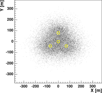
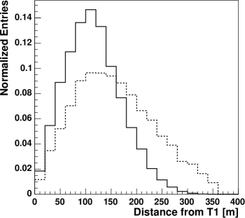
Figure 1: The left panel shows the distribution of the core locations of the triggered $\gamma$-ray-initiated air showers in the plane of the telescopes. For reference, the circles give the location of the 4 VERITAS telescopes. The right panel shows the distribution of the distances of the air shower cores from the central telescope T1 for $\gamma$-ray (solid line) and proton (dashed line) initiated air showers that triggered the experiment.

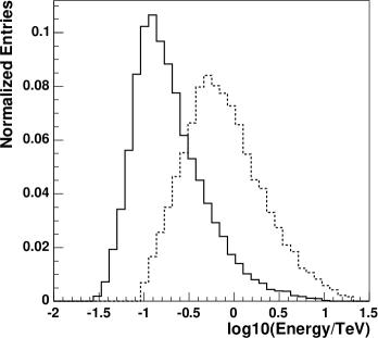
Figure 2: Distribution of the primary energy of photons (solid line) and protons (dashed line) that triggered the telescope array. The photon distribution peaks at $\sim$100 GeV and the proton distribution at $\sim$550 GeV.

The left panel of Fig. 1 shows the distribution of air shower cores of the triggered $\gamma$-rays (the points where the air shower axes intersect the telescope plane). Air showers basically trigger when their cores fall within the air shower array or less than $\sim$150 m away from the outer three telescopes. The right panel of Fig. 1 gives the distribution of the distances of air shower cores from the center of the telescope array for both triggered $\gamma$-rays and protons. The core distributions smoothly approach zero at 350 m from the central telescope, showing that we simulated air showers over a sufficiently large area to produce a realistic air shower dataset. In Fig. 2 we present the distribution of the energies of triggered events for both $\gamma$-rays and protons. The simulations cover sufficiently broad energy ranges, as the distributions approach zero close to the boundaries of the simulated range. The differential detection rate per logarithmic energy interval peaks at about 100 GeV for photons and 550 GeV for protons. We see that proton-initiated events have a substantially higher energy threshold than $\gamma$-ray-initiated events. The latter is a well known consequence of (a) hadronic showers channeling a fraction of their energy into muons and neutrinos via $\pi^{+,-}$-production, and (b) hadronic showers being more irregular than purely electromagnetic showers and thus being more unlikely to generate multi-pixel and multi-telescope coincidences.

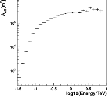
Figure 3: Effective area for detecting cosmic $\gamma$-rays as function of primary energy. Above the threshold region ($>$100 GeV), the effective area increases only slowly with energy.

Fig. 3 presents the effective detection area for $\gamma$-rays. It rises proportional to $E^{4.4}$ in the threshold region ($<$100 GeV) and proportional to $E^{0.27}$ at higher energies ($>$300 GeV).

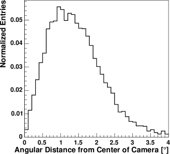
Figure 4: Distribution of the angular distance between the arrival directions of all protons that triggered the experiment and the center of the field of view of the cameras.

The distance of the arrival directions of triggered proton events from the center of the field of view is shown in Fig. 4. At $\sim$4^∘ from the center of the field of view, hardly any protons trigger the telescopes.

3 Reconstruction of Shower Axis

The reconstruction of the air shower direction and core is based on the simple fact that the major axes of the images are projections of the shower axis. In the field of view of the telescopes the major axes intersect at the point corresponding to the arrival direction of the primary particle. In the reference frame of the telescopes, all ellipse-like images point away from the shower core (the intersection of the shower axis and the telescope plane) and the core can again be found at the intersection point of the major axes [11, 12]. If the cosmic $\gamma$-ray source is a point source at a well-known position in the sky, the air shower core can be determined with very high statistical accuracy. One can use the fact that the lines pointing from the location of the source to the centroids of the air shower images point to the air shower core [13]. These lines can be reconstructed with a higher statistical accuracy than the major axes of the ellipse images. If not stated otherwise, we will assume in the following that the source is a point source of known location.

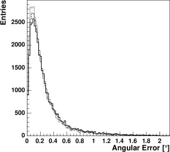
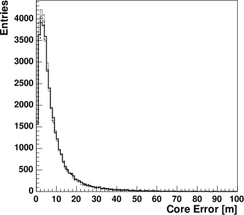
Figure 5: The left panel shows the point spread function for all photon-initiated events that triggered the telescope array. The different line styles show different weighting algorithms. The solid line shows the results for constant weights; the dashed line shows weights proportional to the size parameter, and the dotted line shows a weight that depends on the size, width and length parameters. All three weighting schemes give very similar results. For the best method (dotted line), we get an angular resolution (63% value) of 0.22^∘. The right panel shows the distributions of the error in the core location for all $\gamma$-ray-initiated events. The different line styles correspond to the same weighting schemes as describes for the left side. For the best method (dotted line), we get a core resolution (63% value) of 7.5 m.

In practice, finding the best reconstruction algorithm means combining the information from all telescopes in an optimal way to minimize the statistical error of the direction and core estimates. Here we treat the problem as a $\chi^{2}$-minimization problem. First the direction is determined by finding the point that minimizes the weighted squared distances to the major axes. Subsequently, shower core is reconstructed by minimizing the weighted squared distances to the lines that go through the location of the source and the centroids of the images. Compared to averaging over intersection points from pairs of telescopes, this approach has the advantage that the information about the location and orientation of all telescopes enters the estimate at the same time rather than sequentially. As usual in a $\chi^{2}$-fit, the weights used for combining the information of all images should be inversely proportional to the “squared statistical error” associated with each image. We experimented with three different weighting schemes. The simplest ones use constant weights or weights inversely proportional to the parameter $size$, the sum of the counts of the corresponding image. Furthermore, we scrutinized the mean distances between the major axes (or lines between the source direction and image centroids) and the true direction and core as function of several parameters, i.e., $size$, $width$, $length$, $width/length$, and distance of the telescope to the shower axis $r$. The mean distances indeed scale approximately proportional to $1/size$. After scaling the errors with $1/size$, we still find a rather strong residual dependence on $width$ (not on $width/length$ as one may naively expect as the $width/length$-values characterize the ellipticities of the images). We determined an empirical weighting function that depends on the $size$, $width$ and $length$ parameters. Fig. 5 presents the angular and core resolutions achieved with three weighting schemes. While the more sophisticated weighting schemes improve on the angular and core resolutions, the improvement is very small. Weighting according to the third scheme, we obtain an angular and core resolution (63 % value) of 0.22 ^∘ and 7.5 m, respectively. The lack of a substantial improvement may stem from the fact that the images in the same shower tend to have the same quality, minimizing the effect of the weights. The results agree well with those of an earlier study performed for the HEGRA Cherenkov telescope array [13].

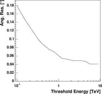
Figure 6: Angular resolution (63% value) as function of threshold energy. The reconstructed energy was used to impose the threshold energy cut. Only events with reconstructed core locations within 150 m from the central telescope were used here. The angular resolution substantially improves above the hardware energy threshold.

The performance improves if high-quality events are selected. Using only events with a reconstructed shower core within 150 m from the central telescope and with a reconstructed energy exceeding 300 GeV we obtain angular and core resolutions of 0.1^∘ and 4.1 m, respectively. Figure 6 shows the angular resolution for different software energy thresholds. The resolution improves with increasing energy threshold and above 1 TeV we obtain a resolution of 0.05^∘. The cut on the core location is critical for obtaining the good results. Without it, more and more events far away from the telescope array trigger the array. At the hardware trigger threshold the cut excludes 24% of the photon initiated events from the analysis.

For extended sources, we do not know the arrival direction of the photons a priori, and the major axes have to be used to determine the shower core location. Rather independent of the applied weighting scheme, the core resolution deteriorates from 7.5 m (4.1 m) for the point source analysis method to 37 m (17 m) for the extended source analysis method (the values in brackets have been determined for a software energy threshold of 300 GeV).

4 Energy Reconstruction

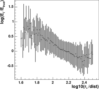
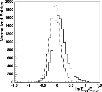
Figure 7: The left panel shows the logarithm of the ratio between reconstructed and true air shower energy as function of the ratio between the distance from a telescope and the dist parameter measured in that telescope. The latter ratio depends somewhat on the height of the shower maximum. The higher (lower) in the atmosphere the shower develops, the larger (smaller) the ratio. One can see that the reconstructed energy is overestimated (underestimated) for showers developing low (high) in the atmosphere. The right side compares the energy resolution achieved with correction (dashed line) and without correction (solid line) for the height of the shower maximum. After (before) correction we get an energy resolution of 22% (28%). The plots include all events for which the reconstructed energy exceeds 100 GeV and for which the reconstructed shower core less than 200 m away from the central telescope.

Together, the atmosphere and the Cherenkov telescopes constitute a fully active calorimeter with sparse sampling. The energy of the primary particle is roughly proportional to the Cherenkov light intensity measured with the telescopes. In the following we discuss only the reconstruction of the primary energy for $\gamma$-rays. We implemented a simple energy reconstruction method (see also [19, 25, 26]). We determined the median and 90%-width-values of the logarithm of the size parameters as function of the primary $\gamma$-ray energy $E$ and distance $r$ from the shower axis. For each telescope with a telescope trigger, an energy estimate is determined by inverting the lookup table. The energy of the primary particle is determined by averaging the energy estimates from all telescope with a telescope trigger. We weight the estimates from each single telescope proportional to one over the square of the statistical uncertainty on the estimate. Combining in this way the energy estimates from different telescopes gives an energy resolution $\sigma_{{\rm ln}{(E_{\rm rec}/E_{\rm true})}}$ of 0.28 for the analysis of point sources and 0.4 for the analysis of extended sources. We focus in the following on the analysis of point sources.
In order to improve on the energy estimate we take into account that the Cherenkov light intensity depends on the height of the shower maximum. Given the stereoscopic air shower data, the height of the shower maximum can be determined. We use the ratio between the distance of a telescope to the shower axis $r$ and the angular distance dist between the centroid of the image and the reconstructed shower direction as an estimate of the shower maximum. For a constant shower maximum we expect that $r$ and dist are roughly proportional to each other and thus that $r$/dist = const. The closer the shower maximum is to the observation level, the further away the image is from the center of the field of view and the larger is the dist value for a given distance from the shower axis, and the smaller is the $r$/dist ratio. The left panel of Fig. 7 shows the logarithm of the ratio between the reconstructed energy and the true energy as function of $r$/dist. Indeed, we see that the simple algorithm severely underestimates (overestimates) the energy for showers with a shower maximum high (low) in the atmosphere. We add a correction that depends on the $r$/dist ratio and the size measured in a telescope. The dependence on the size-parameter takes into account that the correction depends somewhat on the primary energy of the inducing particle. The right panel of Fig. 7 compares the energy resolution achieved with and without the correction. The correction improves the energy resolution $\sigma_{{\rm ln}{(E_{\rm rec}/E_{\rm true})}}$ of the air shower array from 0.28 to 0.22. The performance improves if high-quality events are selected. Using only events with a reconstructed shower core within 150 m from the central telescope and selecting events with a reconstructed energy exceeding 300 GeV we obtain an energy resolution $\sigma_{{\rm ln}{(E_{\rm rec}/E_{\rm true})}}$ of 0.15.

5 Gamma-Hadron Separation

One of the main strengths of Cherenkov telescope experiments is the large collection area on the order of $10^{5}$ m². As a consequence, they achieve unequaled sensitivity for $\gamma$-ray observations on short time scales. However, for longer integration times their sensitivity is limited by fluctuations in the rate of background events and thus increases only with the square root of the observation time. At energies of 100 GeV the air shower background consists of Cosmic Ray hadrons and Cosmic Ray electrons. We only discuss the suppression of the first. Based on today’s technology, electron initiated air showers can only be suppressed based on their isotropic arrival direction. In the following we study only proton-initiated air showers. Protons are expected to make up about 75% of the Cosmic-Ray initiated background. The other 25% are mainly produced by Cosmic Ray He-nuclei. We expect that proton-initiated air showers resemble $\gamma$-ray-initiated air showers more closely than air showers initiated by heavier nuclei.

Normalized Width

We discuss five methods to distinguish between $\gamma$-ray and hadron-initiated air showers (see also the excellent discussion in [27, 28]). The first approach analyzes the width of the air shower images perpendicular to the major axes. Hadron-initiated air showers show significantly “wider” images than $\gamma$-ray-initiated showers owing to the transverse momentum inherent in hadronic interactions. The transverse momentum originates in the non-negligible kinetic energy of the nucleons inside hadronic nuclei and the quarks inside the nucleons. Similar to Aharonian et al. (1997) [11], we use the width parameters measured in all telescopes to derive a $\gamma$-hadron separation parameter. Based on the Monte Carlo dataset, we derive a lookup table of expected median width values, $w_{\rm m}$, and the 90%-widths of the distributions, $w_{90}$, as functions of the size of the image and the distance $r$ of the telescope from the shower axis. Here the median and 90%-width are used rather than the average and the RMS to reduce the impact of outliers in the width distributions. Here and further below, we have used half the dataset for optimizing the method, and the other half to measure its performance.

Given the $w_{\rm m}(r,size)$ and $w_{\rm 90}(r,size)$-values from the lookup table, a “normalized width” value is computed by:

$$w\,\,=\,\,\frac{1}{N_{\rm trig}}\times\left[\sum_{i}^{N_{\rm trig}}\,\frac{width_{\rm i}-w_{\rm m}(r_{\rm i},size_{\rm i})}{w_{90}(r_{\rm i},size_{\rm i})}\right]$$ (1)

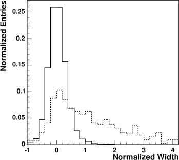
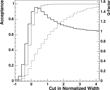
Figure 8: The left panel shows the distribution of the normalized width parameter for photon (solid line) and proton (dashed line) initiated events (three-telescope trigger condition). The right panel shows the photon acceptance $\epsilon_{\gamma}$ (dashed line) and proton acceptance $\epsilon_{\rm p}$ (dashed-dotted line) as function of a cut on the normalized width parameter $w<w_{\rm cut}$. The solid line shows the $Q$-factor. Here it peaks at $Q_{\rm max}\,=$ 1.5.

where the sum runs over all ${N_{\rm trig}}$ telescopes with a telescope trigger, width_i and size_i are the width and size values of the image found in the i^th telescope with a trigger, and $r_{\rm i}$ is the distance of the i^th telescope from the shower axis. The distribution of the normalized width parameter for photons and protons is shown in the left panel of Fig. 8. Accepting events with a normalized width value below a certain cut value w_cut for the analysis, will accept a fraction $\epsilon_{\gamma}$ of $\gamma$-ray-initiated events and a fraction of $\epsilon_{\rm p}$ of proton-initiated events. The $Q$-factor of a $\gamma$-hadron separation method is defined as

$$Q\,\,=\,\,\frac{\epsilon_{\gamma}}{\sqrt{\epsilon_{\rm p}}}$$ (2)

where $\epsilon_{\gamma}$ and $\epsilon_{\rm p}$ are the fractions of photon and hadron initiated events surviving the cut. The $Q$-factor resembles the improvement in signal to noise ratio achieved with a cut, assuming that the noise is dominated by background fluctuations. The values $\epsilon_{\gamma}$, $\epsilon_{\rm p}$ and the $Q$-factor are given as function of the cut value width_cut in the right panel of Fig. 8. We obtain an optimal $Q$-factor of 1.5 for $w_{\rm cut}\,=$ 0.3. Using the more restrictive condition that four rather than three telescopes triggered, improves the performance of the normalized width cut to a maximum $Q$-value of 2.38 for $w_{\rm cut}\,=$ -0.1. The performance of the normalized width cut, as well as that of the $\gamma$-hadron separation methods described in the following paragraphs is summarized in Table 1.

Agreement Between Different Telescopes Regarding the Shower Direction and Core

Krennrich & Lamb (1995) [29] and Hillas (1996) [27] suggested to use the deviation of the major axes from the reconstructed shower direction and/or core location as means to distinguish between photon and hadron-initiated events. The wider and more irregular hadron-initiated showers tend to produce images that do not all point to the arrival direction and core location. We use chi-square values $\chi_{\rm dir}^{2}$ and $\chi_{\rm core}^{2}$ of the direction and core fits, respectively, to differentiate between photons and hadrons. We normalize the chi-square values according to the number of telescopes participating in the fit. We find that the optimal cuts in the chi-square values $\chi_{\rm dir}^{2}$ and $\chi_{\rm core}^{2}$ result in hadron suppressions with $Q$-factors of 1.34 and 1.69 (three-telescope trigger condition) and 1.53 and 2.3 (four-telescope trigger condition), respectively. The cut in $\chi_{\rm core}^{2}$ is very powerful, and achieves a comparable $\gamma$/hadron separation as the cut in the normalized width parameter.

Lateral Cherenkov Light Distribution

The fourth method takes into account that photon and hadron initiated air showers exhibit a different lateral Cherenkov light distribution, and that Cherenkov light pool is more homogeneous for photon initiated air showers than for hadron initiated air showers. We make use of these differences by comparing the energy estimates derived from the information of individual telescopes with the energy derived from the information of all telescopes. Hereby, all energy estimates assume that the primary particle is a photon. We define a reduced chi-square value as follows:

$$\chi_{\rm E}^{2}\,\,=\frac{const}{N_{\rm trig}-1}\times\sum_{i=1}^{N_{\rm trig}}\,\,\frac{{\rm ln}(E_{\rm i}/E_{\rm all})}{\sigma_{{\rm ln}{(E_{\rm i})}}^{\,\,2}}$$ (3)

The sum runs over all telescopes with a trigger, $E_{\rm all}$ is the energy estimate derived from all telescopes, $E_{i}$ is the energy estimate derived from the i^th telescope, and $\sigma_{{\rm ln}{(E_{\rm i})}}$ is the estimated error on ${\rm ln}{(E_{\rm i})}$. Optimizing the cut-value, we find that the $\chi_{\rm E}^{2}$-cut gives maximum $Q$-factors of 1.30 and 1.60 for the three-telescope and four-telescope trigger conditions, respectively.

Making Use of the Temporal Information

Another consequence of the more regular nature of the electromagnetic showers compared to hadronic showers, is that their Cherenkov light front is narrower in time. The VERITAS array of Cherenkov telescopes is equipped with fast FADCs to read out the pixel signals. As fifth $\gamma$-hadron separation method, we compute for each pixel the time at which the signal rose to 50% of its peak, and compute a reduced chi-square value $\chi_{\rm time}^{2}$ as the root mean square (RMS) value of these rise times divided by the degrees of freedom. For the three-telescope and four-telescope trigger conditions, a cut in $\chi_{\rm time}^{2}$ gives $Q$-factors of 1.09 and 1.22, respectively.

Combining the Information of Various Methods

Scatter plots between two of the five $\gamma$-hadron parameters discussed above show that the parameters are not strongly correlated with each other. Cutting in several parameters should result in an improved performance. We apply the likelihood ratio formalism to combine the information from different approaches. We use the $\gamma$-ray and proton distributions of the cut parameters as probability density functions (PDFs). The $\gamma$-hadron separation parameter is then the logarithm of the ratio of the probability that the event is a photon divided by the probability that it is a proton. We define the parameter:

$$\lambda_{1}\,\,=\,\,\sum_{i=1}^{N}\left[{\rm ln}(P_{\rm i}^{\gamma})-{\rm ln}(P_{\rm i}^{\rm p})\right]$$ (4)

where the sum runs over the $N$ $\gamma$-hadron separation methods to be used, and $P_{\rm i}^{\gamma}$ and $P_{\rm i}^{\rm p}$ are the probabilities that photon and proton-initiated air showers produce the observed value of the i^th parameter, respectively. While this approach should give the optimal results if the parameters are indeed completely uncorrelated, we also compute a second parameter which might work better if there is some correlation between the parameters:

$$\lambda_{2}\,\,=\,\,\min_{i=1..N}\left({\rm ln}(P_{\rm i}^{\gamma})-{\rm ln}(P_{\rm i}^{\rm p})\right)$$ (5)

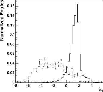
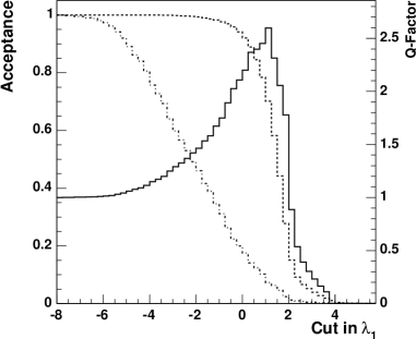
Figure 9: Same as Fig. 8 for the cut $\lambda_{1}(w,\chi_{\rm dir}^{2},\chi_{\rm core}^{2},\chi_{\rm E}^{2})$. The maximum $Q$-factor is 2.60.

Basically, we identify an event as a proton-initiated event if one of the used parameters strongly favors the proton over the photon hypothesis. The performance of several combinations of the separation parameters are given in Table 1. For the three-telescope coincidence condition, we find that combining the information from all five $\gamma$-hadron separation methods improves on the best $Q$-factor 1.7 of a single method, to a $Q$-factor of about 2.6 (see Fig. 9). In the case of the four-telescope trigger condition, the parameter $w$ alone gives $Q\,=$2.4. Combining the information from $w$ and $\chi^{2}_{\rm core}$ improves the performance to a $Q$-factor of 3.6. In all cases, there is little difference between using Equ. (4) or Equ. (5) for combining the information.

Please note that we get very comparable results and almost identical $\gamma$-hadron separation $Q$-factors for the analysis of point sources and extended sources.

Finally, we would like to mention that imposing the four-telescopes trigger condition reduces the number of detected $\gamma$-ray and cosmic ray events. Taking into account the numbers of detected events, the achievable angular resolutions, and the best $Q$-factors, we compute that the signal to noise ratio of a point source detection is by a factor of 1.9 better for the events taken with the four-telescope trigger condition than for all the events taken with the three-telescope trigger condition.

6 Summary and Discussion

We have used a dataset of simulated photon and proton air showers to study the performance of simple event reconstruction methods. Furthermore, we have explored different schemes to improve on the performance of the methods. We have shown that the direction and core reconstruction are insensitive to details of the weighting of the major axis of the individual telescopes. The energy resolution benefits from correcting for the height of the shower maximum. For the analysis of point sources, we get angular, core and energy resolutions of 0.22^∘ (0.1^∘), 7.5 m (4.1 m), and 22% (15%), respectively. The first set of numbers applies to all events that produce a three-telescope trigger. The set of numbers in brackets applies to events with a shower core within 150 m from the central telescope and with a reconstructed energy exceeding 300 GeV. In general, our performance estimates for the VERITAS experiment agree well with the experimentally verified performance of the H.E.S.S. experiment [30].
We have compared different $\gamma$-hadron separation methods and have shown that the information from several parameters can be combined based on the likelihood ratio approach. Compared to a cut in a single $\gamma$-hadron separation parameter, a cut on the likelihood ratio improves the $Q$-factor from 1.7 to 2.6 (three-telescope trigger) and from 2.4 to 3.6 (four-telescope trigger).

It is instructive to compare the relative importance of the hadron and electron backgrounds before and after applying the $\gamma$-hadron separation cuts. Above 30 GeV the BESS energy spectrum for protons impinging on the atmosphere is [31]:

$$\frac{dF_{\rm p}}{dE}\,\,=\,\,9.6\times 10^{-9}(E/1000\,{\rm GeV})^{-2.7}\rm\,cm^{-2}\,s^{-1}\,sr^{-1}\,GeV^{-1}$$ (6)

The 1 GeV-100 GeV electron spectrum measured by HEAT is [32]:

$$\frac{dF_{\rm e}}{dE}\,\,=\,\,1.2\times 10^{-3}\times(E/1\rm\,GeV)^{-1}\times$$

$$\hskip 56.9055pt\left(1+(E/5\,\rm GeV)^{2.3}\right)^{-1}\rm\,cm^{-2}\,s^{-1}\,sr^{-1}\,GeV^{-1}$$ (7)

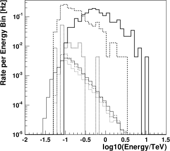
Figure 10: The top three curves show the rate of proton events found in a circular bin of 0.25^∘ radius at the center of the field of view of the telescopes. The top three curves show the proton rate (i) before application of the $\gamma$-hadron separation cut as function of the true proton energy (solid line), (ii) before cut as function of the reconstructed energy (dashed line), and (iii) after cut as function of the reconstructed energy (dotted line). The lower three lines show the same for the electrons rather than protons. One can see that the proton background dominates over the electron background, even after applying the $\gamma$-hadron separation cut. We used here the cut $\lambda_{1}(w,\chi_{\rm dir}^{2},\chi_{\rm core}^{2},\chi_{\rm E}^{2})$.

In Fig. 10 we show the proton and electron trigger rates as function of the true and reconstructed shower energy before and after applying a $\gamma$-hadron separation cut. We used here the three-telescope trigger condition and a $\gamma$-hadron separation cut in $\lambda_{1}(w,\chi_{\rm dir}^{2},\chi_{\rm core}^{2},\chi_{\rm E}^{2})$. As proton-initiated showers produce less Cherenkov light than purely electromagnetic showers, the reconstructed proton energies are on average lower than the true ones. For electrons, there is not such a systematic shift. Notwithstanding this dramatic effect, the hadron background still dominates over the electron-background – even after applying the gamma-hadron separation cut. The result shows that excellent $\gamma$-hadron suppression continues to be of utmost importance for VERITAS and other similar experiments.
                 
Acknowledgements: HK thanks Jim Buckley, Ira Jung, Scott Hughes, Jeremy Perkins, Paul Rebillot and the anonymous referee for fruitful suggestions to improve the text. HK acknowledges support of the DOE through the Outstanding Junior Investigator program. GM acknowledges the support as a Feodor Lynen Fellow of the Alexander von Humboldt foundation.

Table 1: $Q$-factors, photons and proton acceptance and cut value for the $\gamma$-hadron separation methods described in the text.

$\gamma$-hadron sep. parameter	$Q^{a}$	$\epsilon_{\gamma}$ $\left[\%\right]^{a}$	$\epsilon_{\rm p}$ $\left[\%\right]^{a}$	cuta	$Q^{b}$	$\epsilon_{\gamma}$ $\left[\%\right]^{b}$	$\epsilon_{\rm p}$ $\left[\%\right]^{b}$	cutb
w	1.51	89	35	0.3	2.38	46	3.7	-0.1
log($\chi_{\rm dir}^{2})$	1.34	79	35	2.7	1.53	56	13	2.3
log($\chi_{\rm core}^{2})$	1.69	85	25	0.9	2.30	76	11	0.8
log($\chi_{\rm E}^{2}$)	1.30	86	44	-0.1	1.60	57	13	-0.5
log($\chi_{\rm time}^{2})$	1.09	85	61	1.1	1.22	83	47	1.1
$\lambda_{1}(w,\chi_{\rm core}^{2})$	2.27	78	12	0.625	3.59	62	2.9	1.375
$\lambda_{2}(w,\chi_{\rm core}^{2})$	2.31	76	11	0.125	3.27	79	6	0.125
$\lambda_{1}(w,\chi_{\rm core}^{2},\chi_{\rm E}^{2})$	2.22	89	18	0.375	3.09	83	8.8	1.125
$\lambda_{2}(w,\chi_{\rm core}^{2},\chi_{\rm E}^{2})$	2.24	63	8	0.125	3.99	68	2.9	0.125
$\lambda_{1}(w,\chi_{\rm dir}^{2},\chi_{\rm core}^{2},\chi_{\rm E}^{2})$	2.60	70	7.3	1.125	3.07	82	7	1.375
$\lambda_{2}(w,\chi_{\rm dir}^{2},\chi_{\rm core}^{2},\chi_{\rm E}^{2})$	2.59	53	4.1	0.125	3.72	81	4.7	-0.125
$\lambda_{1}(w,\chi_{\rm dir}^{2},\chi_{\rm core}^{2},\chi_{\rm E}^{2},\chi_{\rm time}^{2})$	2.40	68	8	1.125	3.16	64	4	2.125
$\lambda_{2}(w,\chi_{\rm dir}^{2},\chi_{\rm core}^{2},\chi_{\rm E}^{2},\chi_{\rm time}^{2})$	2.41	65	7	-0.125	3.17	59	3.5	0.125

^aTrigger condition: three or four triggered telescopes.

^bTrigger condition: four triggered telescopes.

References

- [1] Hillas, A. M. 1985, Proc. 19th ICRC (La Jolla), 3, 445
- [2] Weekes, T. C., Cawley, M. F., Fegan, D. J., et al. 1989, ApJ, 342, 379
- [3] Weekes, T. C. 2003, “Very high energy gamma-ray astronomy”, Bristol (Philadelphia), Institute of Physics Pub.
- [4] Aharonian, F. A. 2004, “Very high energy cosmic gamma radiation: a crucial window on the extreme universe”, Published Singapore (Hong Kong), World Scientific
- [5] Krawczynski, H. 2005, Procs. of the “Blazar Variability Workshop II: Entering the GLAST Era”, April 10-12, 2005, Miami, Florida, USA [astro-ph/0508621]
- [6] Aharonian, F. A., Akhperjanian, A. G., Aye, K. M., et al. 2005, Science, 307, 1938
- [7] Weekes, T. C., Badran, H., Biller, S. D., et al. 2002, APh, 17, 221
- [8] Hinton, J. A., for the H.E.S.S. Collaboration 2004, New Astron. Rev., 48, 331
- [9] Bastieri, D., Bavikadi, R., Bigongiari, C. 2004, In Procs. of the 6th International Symposium ”Frontiers of Fundamental and Computational Physics” (FFP6), Udine (Italy), Sep. 26-29, 2004
- [10] Kawachi, A., Hayami, Y., Jimbo, J., et al. 2001, APh, 14, 261
- [11] Aharonian, F. A., Hofmann, W., Konopelko, A. K., Völk, H. 1997, APh, 6, 343
- [12] Krennrich, F., Akerlof, C. W., Buckley, J. H., et al. 1998, APh, 8, 213
- [13] Hofmann, W., Jung, I., Konopelko, A., Krawczynski, H., Lampeitl, H., Pühlhofer, G. 1999, APh, 12, 135
- [14] Le Bohec, S., Degrange, B., Punch, M., et al. 1998, NIMA, 416, 475
- [15] Ulrich, M., Daum, A., Hermann, G., Hofmann, W. 1998, J. Phys. G., 24, 883
- [16] Le Bohec, S., Duke, C., Jordan, P., et al. 2005, APh, 24, 26
- [17] Daum, A., Hermann, G., Hess, M., et al. 1997, APh, 8, 1
- [18] Aharonian, F. A., Akhperjanian, A. G., Barrio, J. A., et al. 1999, APh, 10, 21
- [19] Aharonian, F. A., Akhperjanian, A. G., Barrio, J. A., et al. 1999, A&A, 342, 69
- [20] Aharonian, F. A. 2005, “Next generation of IACT arrays: scientific objectives versus energy domains”, In Procs.: “Towards a Network of Atmospheric Cherenkov Detectors VII”, 2005, Palaiseau, France”, [astro-ph/0511139]
- [21] Krennrich, F., Biller, S. D., Bond, I. H., et al. 1999, ApJ, 511, 149
- [22] Konopelko, A., Aharonian, F., Hemberger, M. 1999, J. Phys. G, 25, 1989
- [23] Kosack, K., Bond, H. M., Boyle, I. H., et al. 2004, ApJL, 608, 97
- [24] Kertzman, M. P., Sembroski, G. H. 1994, NIMA, 343, 629
- [25] Aharonian, F. A., Akhperjanian, A. G., Barrio, J. A. 1999, A&A, 349, 11
- [26] Aharonian, F. A., Akhperjanian, A. G., Barrio, J. A. 2001, A&A, 366, 62
- [27] Hillas, A. M. 1996, SpScRev, 75, 17
- [28] Fegan, D. J. 1996, SpScRev, 75 137
- [29] Krennrich, F., Lamb, D. 1995, Exp. Astronomy, 6, 285
- [30] Aharonian, F., Akhperjanian, A. G., Aye, K.-M., et al. 2005, A&A, 430, 865
- [31] Sanuki, T., Motoki, M., Matsumoto, H. et al. 2000, ApJ, 545, 1135
- [32] DuVernois, M. A., Barwick, S. W., Beatty, J. J., et al. 2001 ApJ, 559, 296