TIME-DEPENDENT STOCHASTIC PARTICLE ACCELERATION IN ASTROPHYSICAL PLASMAS: EXACT SOLUTIONS INCLUDING MOMENTUM-DEPENDENT ESCAPE

Abstract

Stochastic acceleration of charged particles due to interactions with magnetohydrodynamic (MHD) plasma waves is the dominant process leading to the formation of the high-energy electron and ion distributions in a variety of astrophysical systems. Collisions with the waves influence both the energization and the spatial transport of the particles, and therefore it is important to treat these two aspects of the problem in a self-consistent manner. We solve the representative Fokker-Planck equation to obtain a new, closed-form solution for the time-dependent Green’s function describing the acceleration and escape of relativistic ions interacting with Alfvén or fast-mode waves characterized by momentum diffusion coefficient $D(p)\propto p^{q}$ and mean particle escape timescale $t_{\rm esc}(p)\propto p^{q-2}$, where $p$ is the particle momentum and $q$ is the power-law index of the MHD wave spectrum. In particular, we obtain solutions for the momentum distribution of the ions in the plasma and also for the momentum distribution of the escaping particles, which may form an energetic outflow. The general features of the solutions are illustrated via examples based on either a Kolmogorov or Kraichnan wave spectrum. The new expressions complement the results obtained by Park and Petrosian, who presented exact solutions for the hard-sphere scattering case ($q=2$) in addition to other scenarios in which the escape timescale has a power-law dependence on the momentum. Our results have direct relevance for models of high-energy radiation and cosmic-ray production in astrophysical environments such as $\gamma$-ray bursts, active galaxies, and magnetized coronae around black holes. In particular, we outline an application of the new results to black-hole sources that produce outflows of relativistic hadrons, with associated predictions that can be tested using GLAST.

1 INTRODUCTION

Observations of high-energy radiation from a variety of astrophysical sources imply the presence of significant populations of nonthermal (often relativistic) particles. Much of the observational data is characterized by strong variability on very short timescales. Nonthermal distributions are naturally produced via the Fermi process, in which particles interact with scattering centers moving systematically and/or randomly. The first-order Fermi mechanism treats particle acceleration in converging flows, such as shocks, and is thought to be important at the Earth’s bow shock, in certain classes of solar flares, for cosmic-ray acceleration by supernova remnants, and in sources with relativistic outflows, including blazars and $\gamma$-ray bursts (for reviews, see Blandford & Eichler, 1987; Kirk, 1994). The second-order process, as it was originally conceived by Fermi, involved the stochastic acceleration of particles scattering with randomly moving magnetized clouds (Fermi, 1949). Later refinements of this idea replaced the magnetized clouds with magnetohydrodynamic (MHD) waves (e.g., Melrose, 1980). The second-order, stochastic Fermi process now finds application in a wide range of astrophysical settings, including solar flares (Miller et al., 1990; Liu et al., 2004a), clusters of galaxies (Schlickeiser et al., 1987; Petrosian, 2001; Brunetti et al., 2004), the Galactic center (Liu et al., 2004b; Atoyan & Dermer, 2004), and $\gamma$-ray bursts (Waxman, 1995; Dermer & Humi, 2001).

The standard approach to modeling the acceleration of nonthermal particles via interactions with MHD waves involves obtaining the solution to a steady-state transport equation that incorporates treatments of systematic and stochastic Fermi acceleration, radiative losses, and particle escape (e.g., Schlickeiser, 1984; Schlickeiser & Steinacker, 1989; Liu et al., 2006). However, the prevalence of variability on short timescales in many sources calls into question the validity of the steady-state interpretation. Park & Petrosian (1995) provided a comprehensive review of the various time-dependent solutions that have been derived in the past 30 years. In most cases, it is assumed that the momentum diffusion coefficient, $D(p)$, and the mean particle escape timescale, $t_{\rm esc}(p)$, have power-law dependences on the particle momentum $p$. Although the set of existing solutions covers a broad range of possible values for the associated power-law indices, there are certain physically interesting cases for which no analytical solution is currently available. For example, Dermer et al. (1996) have shown that for the stochastic acceleration of relativistic particles due to resonant interactions with plasma waves in black-hole magnetospheres, one obtains $D(p)\propto p^{q}$ and $t_{\rm esc}(p)\propto p^{q-2}$, where $q$ is the index of the wavenumber distribution (see § 2). The analytical solution for the time-dependent Green’s function in this situation is of particular physical interest, but it has not appeared in the previous literature. This has motivated us to reexamine the associated Fokker-Planck transport equation for this case, and to obtain a new family of closed-form solutions for the secular Green’s function. The resulting expression, describing the evolution of an initially monoenergetic particle distribution, complements the set of solutions discussed by Park & Petrosian (1995). Our primary goal in this paper is to present a detailed derivation of the exact analytical solution and to demonstrate some of its key properties. Detailed applications of our results to the modeling of particle acceleration in black-hole accretion coronae and other astrophysical environments will be presented in a separate paper.

The remainder of the paper is organized as follows. In § 2 we review the fundamental equations governing the acceleration of charged particles interacting with plasma waves. The transport equation is solved in § 3 to obtain the time-dependent Green’s function, and illustrative results are presented in § 4. The astrophysical implications of our work are summarized in § 5, and additional mathematical details are provided in the Appendix.

2 FUNDAMENTAL EQUATIONS

Charged particles in turbulent astrophysical plasmas are expected to be accelerated via interactions with whistler, fast-mode, and Alfvén waves propagating in the magnetized gas. Here we consider a simplified isotropic description of the wave energy distribution, denoted by $W(k)$, where $W(k)dk$ represents the energy density due to waves with wavenumber between $k$ and $k+dk$. The transport formalism we consider assumes a power-law distribution for the wave-turbulence spectrum, which implies definite relations between the momentum diffusion coefficient and the momentum-dependent escape timescale (e.g., Melrose, 1974; Schlickeiser, 1989a, b; Dermer et al., 1996). MHD waves injected over a narrow range of wavenumber cascade to larger wavenumbers, forming a Kolmogorov or Kraichnan power spectrum over the inertial range with $W(k)\propto k^{-q}$, where $q=5/3$ and $q=3/2$ for the Kolmogorov and Kraichnan cases, respectively (e.g., Zhou & Matthaeus, 1990). The specific forms we will adopt for the transport coefficients in § 2.2 are based on the physics of the resonant scattering processes governing the wave-particle interactions (see Dermer et al., 1996). We assume that the nonthermal particle distribution is isotropic, and focus on a detailed treatment of the propagation of particles in momentum space due to wave-particle interactions. The spatial aspects of the transport (i.e., the confinement of the particles in the acceleration region) will be treated in an approximate manner using a momentum-dependent escape term.

2.1 Transport Equation

The fundamental transport equation describing the propagation of particles in the momentum space can be written in the flux-conservation form (e.g., Becker, 1992; Schlickeiser, 1989a, b)

$${\partial f\over\partial t}=-{1\over p^{2}}{\partial\over\partial p}\left\{p^{2}\left[A(p)\,f-D(p){\partial f\over\partial p}\right]\right\}-{f\over t_{\rm esc}(p)}+{S(p,t)\over 4\pi p^{2}}\ ,$$ (1)

where $p$ is the particle momentum, $f(p,t)$ is the particle distribution function, $D(p)$ denotes the momentum diffusion coefficient, $t_{\rm esc}(p)$ is the mean escape time, $S(p,t)$ represents particle sources, and $A(p)$ describes any additional, systematic acceleration or loss processes, such as shock acceleration or synchrotron/inverse-Compton emission. The quantity in square brackets in equation (1) describes the flux of particles through the momentum space (Tademaru et al., 1971), and the source term is defined so that $S(p,t)\,dp\,dt$ gives the number of particles injected into the plasma per unit volume between times $t$ and $t+dt$ with momenta between $p$ and $p+dp$. The total particle number density $n(t)$ and energy density $U(t)$ of the distribution $f(p,t)$ are computed using

$$n(t)=\int_{0}^{\infty}4\pi\,p^{2}\,f(p,t)\,dp\ ,\ \ \ \ \ U(t)=\int_{0}^{\infty}4\pi\,\epsilon\,p^{2}\,f(p,t)\,dp\ ,$$ (2)

where the particle kinetic energy $\epsilon$ is related to the Lorentz factor $\gamma$ and the particle momentum $p$ by

$$\epsilon=(\gamma-1)\,mc^{2}\ ,\ \ \ \ \ \gamma=\left({p^{2}\over m^{2}c^{2}}+1\right)^{1/2}\ ,$$ (3)

and $m$ and $c$ denote the particle rest mass and the speed of light, respectively.

Rather than solve equation (1) directly to determine $f(p,t)$ for a given source term $S(p,t)$, it is more instructive to first solve for the Green’s function, $f_{{}_{\rm G}}(p_{0},p,t_{0},t)$, which satisfies the equation

$${\partial f_{{}_{\rm G}}\over\partial t}=-{1\over p^{2}}{\partial\over\partial p}\left\{p^{2}\left[A(p)\,f_{{}_{\rm G}}-D(p){\partial f_{{}_{\rm G}}\over\partial p}\right]\right\}-{f_{{}_{\rm G}}\over t_{\rm esc}(p)}+{\delta(p-p_{0})\,\delta(t-t_{0})\over 4\pi p_{0}^{2}}\ ,$$ (4)

where $p_{0}$ is the initial momentum and $t_{0}$ is the initial time. The source term in this equation corresponds to the injection of a single particle per unit volume with momentum $p_{0}$ at time $t_{0}$. The particle number and energy densities associated with the Green’s function are given by

$$n_{{}_{\rm G}}(t)=\int_{0}^{\infty}4\pi\,p^{2}\,f_{{}_{\rm G}}(p_{0},p,t_{0},t)\,dp\ ,\ \ \ \ \ U_{{}_{\rm G}}(t)=\int_{0}^{\infty}4\pi\,\epsilon\,p^{2}\,f_{{}_{\rm G}}(p_{0},p,t_{0},t)\,dp\ .$$ (5)

Once the Green’s function solution has been determined, the particular solution associated with an arbitrary source distribution $S(p,t)$ can be computed using the integral convolution (e.g., Becker, 2003)

$$f(p,t)=\int_{0}^{t}\int_{0}^{\infty}f_{{}_{\rm G}}(p_{0},p,t_{0},t)\,S(p_{0},t_{0})\,dp_{0}\,dt_{0}\ ,$$ (6)

where we have assumed that the particle injection begins at time $t=0$ and no particles are present in the plasma for $t<0$.

2.2 Transport Coefficients

In Appendix A.1, we demonstrate that for arbitrary particle energies, the mean rate of change of the particle momentum due to stochastic acceleration is related to the momentum diffusion coefficient $D(p)$ via

$$\Big{\langle}{dp\over dt}\Big{\rangle}\Big{|}_{\rm stoch}={1\over p^{2}}{d\over dp}\left(p^{2}D\right)\ .$$ (7)

The corresponding result for the mean rate of change of the kinetic energy is (see Appendix A.2 and Miller & Ramaty, 1989)

$$\Big{\langle}{d\epsilon\over dt}\Big{\rangle}\Big{|}_{\rm stoch}={1\over p^{2}}{d\over dp}\left(p^{2}vD\right)\ ,$$ (8)

where $v$ is the particle speed. If the MHD wave spectrum has the power-law form $W\propto k^{-q}$ associated with Alfvén and fast-mode waves, then the momentum dependences of the diffusion coefficient $D(p)$ and the mean escape time $t_{\rm esc}(p)$ describing the resonant pitch-angle scattering of relativistic particles are given by (e.g., Dermer et al., 1996; Miller & Ramaty, 1989)

$$D(p)=D_{*}\,m^{2}c^{2}\left({p\over mc}\right)^{q}\ ,\ \ \ \ \ \ \ t_{\rm esc}(p)=t_{*}\left({p\over mc}\right)^{q-2}\ ,$$ (9)

where $D_{*}\propto{\rm s}^{-1}$ and $t_{*}\propto{\rm s}$ are constants. We shall focus on transport scenarios with $q\leq 2$, so that $t_{\rm esc}$ is either a decreasing or constant function of the momentum $p$. In order to maintain the physical validity of the escape-timescale approach used here, we must require that $t_{\rm esc}$ exceed the light-crossing time $L/c$ for a source with size $L$. This implies a fundamental upper limit to the particle momentum when $q<2$.

By combining equations (7) and (9), we find that the mean rate of change of the momentum for relativistic particles accelerated stochastically by MHD waves is given by

$$\Big{\langle}{dp\over dt}\Big{\rangle}\Big{|}_{\rm stoch}=(q+2)\,D_{*}\,mc\left({p\over mc}\right)^{q-1}\ .$$ (10)

For simplicity, we shall assume that the momentum dependence of the additional, systematic loss/acceleration processes appearing in the transport equation (1), described by the coefficient $A(p)$, mimics that of the stochastic acceleration (eq. [10]). We therefore write

$$A(p)=A_{*}\,mc\left({p\over mc}\right)^{q-1}\ ,$$ (11)

where the constant $A_{*}\propto{\rm s}^{-1}$ determines the positive (negative) rate of systematic acceleration (losses). Note that this formulation precludes the treatment of loss processes with a quadratic energy dependence (e.g., inverse-Compton or synchrotron) since that would imply $q=3$, which is outside the range considered here. However, first-order Fermi acceleration at a shock or energy losses due to Coulomb collisions can be treated by setting $q=2$ with $A_{*}$ either positive or negative, respectively. This suggests that the results obtained here are relevant primarily for the transport of energetic ions. However, even in this application one needs to bear in mind that synchrotron and inverse-Compton losses will become dominant at sufficiently high energies (e.g., Schlickeiser, 1984; Schlickeiser & Steinacker, 1989; Liu et al., 2006).

It is convenient to transform to the dimensionless momentum and time variables $x$ and $y$, defined by

$$x\equiv{p\over mc}\ ,\ \ \ \ \ \ \ y\equiv D_{*}\,t\ ,$$ (12)

in which case the transport equation (4) for the Green’s function becomes

$${\partial f_{{}_{\rm G}}\over\partial y}={1\over x^{2}}{\partial\over\partial x}\left(x^{2+q}\,{\partial f_{{}_{\rm G}}\over\partial x}\right)-{a\over x^{2}}{\partial\over\partial x}\left(x^{1+q}\,f_{{}_{\rm G}}\right)-\theta\,x^{2-q}\,f_{{}_{\rm G}}+{\delta(x-x_{0})\,\delta(y-y_{0})\over 4\pi m^{3}c^{3}x_{0}^{2}}\ ,$$ (13)

where

$$x_{0}\equiv{p_{0}\over mc}\ ,\ \ \ \ \ \ \ y_{0}\equiv D_{*}\,t_{0}\ ,$$ (14)

and we have introduced the dimensionless constants

$$a\equiv{A_{*}\over D_{*}}\ ,\ \ \ \ \ \ \ \theta\equiv{1\over D_{*}\,t_{*}}\ .$$ (15)

Note that $x$ equals the particle Lorentz factor in applications involving ultrarelativistic particles. The constant $a$ describes the relative importance of systematic gains or losses compared with the stochastic process.

2.3 Fokker-Planck Equation

Additional physical insight can be obtained by reorganizing equation (13) in the Fokker-Planck form

$${\partial N_{{}_{\rm G}}\over\partial y}={\partial^{2}\over\partial x^{2}}\left(x^{q}\,N_{{}_{\rm G}}\right)-{\partial\over\partial x}\left[(q+2+a)\,x^{q-1}\,N_{{}_{\rm G}}\right]-\theta\,x^{2-q}\,N_{{}_{\rm G}}+{\delta(x-x_{0})\,\delta(y-y_{0})}\ ,$$ (16)

where we have defined the Green’s function number distribution $N_{{}_{\rm G}}$ using

$$N_{{}_{\rm G}}(x_{0},x,y_{0},y)\equiv 4\pi\,m^{3}c^{3}\,x^{2}\,f_{{}_{\rm G}}(x_{0},x,y_{0},y)\ .$$ (17)

The Fokker-Planck coefficients appearing in equation (16), which describe the evolution of the particle distribution due to the influence of stochastic and systematic processes, are given by (Reif, 1965)

$${1\over 2}{d\sigma^{2}\over dy}=x^{q}\ ,\ \ \ \ \ \Big{\langle}{dx\over dy}\Big{\rangle}=(q+2+a)\,x^{q-1}\ ,$$ (18)

where the first coefficient describes the “broadening” of the distribution due to momentum space diffusion, and the second represents the mean “drift” of the particles (i.e., the average acceleration rate).

Equation (16) is equivalent to equation (49) from Park & Petrosian (1995) if we set their parameters $a_{\rm pp}=2+a$ and $s_{\rm pp}=q-2$, where $s_{\rm pp}$ denotes the power-law index describing the momentum dependence of the escape timescale. Our particular choice for $s_{\rm pp}$ reflects the physics of the resonant wave-particle interactions, as represented by equations (9). The Fokker-Planck form of equation (16) clearly reveals the fundamental nature of the transport process. In particular, we note that in the limit $a\to 0$, the drift coefficient $\langle dx/dy\rangle$ reduces to the purely stochastic result (eq. [10]), as expected when systematic gains/losses are excluded from the problem. The total number and energy densities are computed in terms of $N_{{}_{\rm G}}$ using (cf. eq. [5])

$$n_{{}_{\rm G}}(y)=\int_{0}^{\infty}N_{{}_{\rm G}}(x_{0},x,y_{0},y)\,dx\ ,\ \ \ \ \ U_{{}_{\rm G}}(y)=\int_{0}^{\infty}\epsilon\,x\,N_{{}_{\rm G}}(x_{0},x,y_{0},y)\,dx\ ,$$ (19)

where (see eq. [3])

$$\epsilon=mc^{2}\left[\left(x^{2}+1\right)^{1/2}-1\right]\ .$$ (20)

Since the physical situation considered here corresponds to the injection of a single particle per unit volume at “time” $y=y_{0}$, it follows that $n_{{}_{\rm G}}(y_{0})=1$.

3 SOLUTION FOR THE GREEN’S FUNCTION

The result obtained for the Green’s function number distribution $N_{{}_{\rm G}}$ has two important special cases depending on whether $q=2$ or $q<2$. Park & Petrosian (1995) obtained the exact solution to equation (16) for the hard sphere case (Ramaty, 1979) with $q=2$ and their parameter $s_{\rm pp}=0$, corresponding to a momentum-independent escape timescale. In this section we derive the exact solution to the time-dependent problem with $q<2$ and $s_{\rm pp}=q-2$, which describes the physics of the wave-particle interactions (see eqs. [9]).

3.1 Laplace Transformation

We define the Laplace transformation of $N_{{}_{\rm G}}$ using

$$L(x_{0},x,s)\equiv\int_{0}^{\infty}e^{-sy}\,N_{{}_{\rm G}}(x_{0},x,y_{0},y)\,dy\ .$$ (21)

By operating on the Fokker-Planck equation (16) with $\int_{0}^{\infty}e^{-sy}\,dy$, we obtain

$${d^{2}\over dx^{2}}\left(x^{q}\,L\right)-{d\over dx}\left[(q+2+a)\,x^{q-1}\,L\right]-\theta\,x^{2-q}\,L-sL=-e^{-sy_{0}}\,\delta(x-x_{0})\ ,$$ (22)

or, equivalently,

$${d^{2}L\over dx^{2}}+\left({q-2-a\over x}\right){dL\over dx}+\left[{(1-q)(2+a)\over x^{2}}-{\theta\over x^{2q-2}}-{s\over x^{q}}\right]\,L=-{e^{-sy_{0}}\,\delta(x-x_{0})\over x^{q}}\ .$$ (23)

This equation can be transformed into standard form by introducing the new momentum variables

$$z(x)\equiv{2\sqrt{\theta}\over 2-q}\ x^{2-q}\ ,\ \ \ \ \ z_{0}(x_{0})\equiv{2\sqrt{\theta}\over 2-q}\ x_{0}^{2-q}\ .$$ (24)

After some algebra, we find that the equation for $L$ now becomes

$$z^{2}\,{d^{2}L\over dz^{2}}+{a+1\over q-2}\,z\,{dL\over dz}+\left[{(1-q)(2+a)\over(2-q)^{2}}-{z^{2}\over 4}-{sz\over c_{0}(2-q)^{2}}\right]\,L=-{c_{0}\,e^{-sy_{0}}\,\delta(z-z_{0})\over 2-q}\,\left({z\over c_{0}}\right)^{(3-2q)/(2-q)}\ ,$$ (25)

where

$$c_{0}\equiv{2\sqrt{\theta}\over 2-q}\ .$$ (26)

The solutions to equation (25) obtained for $z\neq z_{0}$ that satisfy the high- and low-energy boundary conditions are given by

$$L(z_{0},z,s)=e^{-z/2}\,z^{(a+2)/(2-q)}\,\cases{A\,U(\alpha,\beta,z)\ ,&$z\geq z_{0}$ \ ,\cr B\,M(\alpha,\beta,z)\ ,&$z\leq z_{0}$ \ ,\cr}$$ (27)

where $M$ and $U$ denote the confluent hypergeometric functions (Abramowitz & Stegun, 1970), and

$$\alpha\equiv{s+(a+3)\sqrt{\theta}\over 2(2-q)\sqrt{\theta}}\ ,\ \ \ \ \ \ \ \beta\equiv{a+3\over 2-q}\ .$$ (28)

The constants $A$ and $B$ appearing in equation (27) are determined by ensuring that the function $L$ is continuous at $z=z_{0}$, and that it also satisfies the derivative jump condition

$$\lim_{\varepsilon\to 0}{dL\over dz}\bigg{|}_{z_{0}-\varepsilon}^{z_{0}+\varepsilon}=-{c_{0}\,e^{-sy_{0}}\over(2-q)\,z_{0}^{2}}\,\left({z_{0}\over c_{0}}\right)^{(3-2q)/(2-q)}={-e^{-sy_{0}}\over 2\,x_{0}\sqrt{\theta}}\ ,$$ (29)

obtained by integrating the transport equation (25) with respect to $z$ in a small range around the source momentum $z_{0}$.

The constant $B$ can be eliminated by combining the continuity and derivative jump conditions. After some algebra, the solution obtained for $A$ is

$$A=-\,{e^{-sy_{0}}\,e^{z_{0}/2}\,z_{0}^{(a+2)/(q-2)}\,M(\alpha,\beta,z_{0})\over 2\,x_{0}\sqrt{\theta}\,W(z_{0})}\ ,$$ (30)

where $W(z)$ denotes the Wronskian, defined by

$$W(z)\equiv M(\alpha,\beta,z){d\over dz}U(\alpha,\beta,z)-U(\alpha,\beta,z){d\over dz}M(\alpha,\beta,z)\ .$$ (31)

Using equation (13.1.22) from Abramowitz & Stegun (1970), we find that $W$ is given by the exact expression

$$W(z)=-\,{\Gamma(\beta)\,z^{-\beta}\,e^{z}\over\Gamma(\alpha)}\ ,$$ (32)

which can be combined with equation (30) and the continuity relation to obtain

$$A={\Gamma(\alpha)\,z_{0}^{\beta+(a+2)/(q-2)}\,e^{-sy_{0}}\,e^{-z_{0}/2}\,M(\alpha,\beta,z_{0})\over 2\,x_{0}\sqrt{\theta}\,\Gamma(\beta)}\ ,$$ (33)

$$B={\Gamma(\alpha)\,z_{0}^{\beta+(a+2)/(q-2)}\,e^{-sy_{0}}\,e^{-z_{0}/2}\,U(\alpha,\beta,z_{0})\over 2\,x_{0}\sqrt{\theta}\,\Gamma(\beta)}\ .$$ (34)

The final solution for the Laplace transformation $L$ can therefore be written as

$$L(z_{0},z,s)={\Gamma(\alpha)\,z_{0}^{\beta}\over\Gamma(\beta)\,2\,x_{0}\sqrt{\theta}}\,\left({z\over z_{0}}\right)^{(a+2)/(2-q)}\,e^{-sy_{0}}\,e^{-(z+z_{0})/2}\,M(\alpha,\beta,z_{\rm min})\,U(\alpha,\beta,z_{\rm max})\ ,$$ (35)

where

$$z_{\rm min}\equiv\min(z,z_{0})\ ,\ \ \ \ \ \ \ z_{\rm max}\equiv\max(z,z_{0})\ .$$ (36)

3.2 Inverse Transformation

Figure 1: Integration contour $C$ used to evaluate equation (37).

The solution for the Green’s function $N_{{}_{\rm G}}$ can be found using the complex Mellin inversion integral, which states that

$$N_{{}_{\rm G}}(z_{0},z,y_{0},y)={1\over 2\pi i}\int_{\gamma-i\infty}^{\gamma+i\infty}e^{sy}\,L(z_{0},z,s)\,ds\ ,$$ (37)

where $\gamma$ is chosen so that the line ${\rm Re}\,s=\gamma$ lies to the right of any singularities in the integrand. The singularities are simple poles located where $|\Gamma(\alpha)|\to\infty$, which corresponds to $\alpha=-n$, with $n=0,1,2,\ldots$ Equation (28) therefore implies that there are an infinite number of poles situated along the real axis at $s=s_{n}$, where

$$s_{n}=\left[2\,(q-2)\,n-a-3\right]\sqrt{\theta}\ ,\ \ \ n=0,1,2,\ldots$$ (38)

We can therefore employ the residue theorem to write

$$\oint e^{sy}\,L(z_{0},z,s)\,ds=2\pi i\sum_{n=0}^{\infty}\ {\rm Res}(s_{n})\ ,$$ (39)

where $C$ is the closed integration contour indicated in Figure 1 and ${\rm Res}(s_{n})$ denotes the residue associated with the pole at $s=s_{n}$. Based on asymptotic analysis, we conclude that the contribution to the integral due to the curved portion of the contour vanishes in the limit $R\to\infty$, and consequently we can combine equations (37) and (39) to obtain

$$N_{{}_{\rm G}}(z_{0},z,y_{0},y)=\sum_{n=0}^{\infty}\ {\rm Res}(s_{n})\ .$$ (40)

Hence we need only evaluate the residues in order to determine the solution for the Green’s function.

3.3 Evaluation of the Residues

The residues associated with the simple poles at $s=s_{n}$ are evaluated using the formula (e.g., Butkov, 1968)

$${\rm Res}(s_{n})=\lim_{s\to s_{n}}(s-s_{n})\ e^{sy}\,L(z_{0},z,s)\ .$$ (41)

Since the poles are associated with the function $\Gamma(\alpha)$ in equation (35), we will need to make use of the identity

$$\lim_{s\to s_{n}}(s-s_{n})\ \Gamma(\alpha)={(-1)^{n}\over n!}\,2\,(2-q)\,\sqrt{\theta}\ ,$$ (42)

which follows from equations (28) and (38). Combining equations (35), (41), and (42), we find that the residues are given by

$${\rm Res}(s_{n})={(-1)^{n}\,(2-q)\,e^{s_{n}(y-y_{0})}\,z_{0}^{\beta}\over n!\,\Gamma(\beta)\,x_{0}}\,\left({z\over z_{0}}\right)^{(a+2)/(2-q)}\,e^{-(z+z_{0})/2}\,M(-n,\beta,z_{\rm min})\,U(-n,\beta,z_{\rm max})\ .$$ (43)

Based on equations (13.6.9) and (13.6.27) from Abramowitz & Stegun (1970), we note that the confluent hypergeometric functions appearing in this expression reduce to Laguerre polynomials, and therefore our result for the residue can be rewritten after some simplification as

$${\rm Res}(s_{n})={n!\,e^{s_{n}(y-y_{0})}\,z_{0}^{\beta}\,(2-q)\over\Gamma(\beta+n)\,x_{0}}\,\left({z\over z_{0}}\right)^{(a+2)/(2-q)}\,e^{-(z+z_{0})/2}\,P_{n}^{(\beta-1)}(z)\,P_{n}^{(\beta-1)}(z_{0})\ ,$$ (44)

where $P_{n}^{(\beta-1)}(z)$ denotes the Laguerre polynomial.

3.4 Closed-Form Expression for the Green’s Function

The result for the Green’s function number distribution $N_{{}_{\rm G}}$ is obtained by summing the residues (see eq. [40]), which yields

$$N_{{}_{\rm G}}(z_{0},z,y_{0},y)=\sum_{n=0}^{\infty}\ {n!\,e^{s_{n}(y-y_{0})}\,z_{0}^{\beta}\,(2-q)\over\Gamma(\beta+n)\,x_{0}}\,\left({z\over z_{0}}\right)^{(a+2)/(2-q)}\,e^{-(z+z_{0})/2}\,P_{n}^{(\beta-1)}(z)\,P_{n}^{(\beta-1)}(z_{0})\ .$$ (45)

This convergent sum is a useful expression for the Green’s function. However, further progress can be made by employing the bilinear generating function for the Laguerre polynomials, given by equation (8.976) from Gradshteyn & Ryzhik (1980). After some algebra, we find that the general closed-form solution can be written in the form

$$N_{{}_{\rm G}}(x_{0},x,y_{0},y)={2-q\over x_{0}}\left({x\over x_{0}}\right)^{(a+1)/2}\,{\sqrt{zz_{0}\xi}\over 1-\xi}\ \exp\left[-{(z+z_{0})(1+\xi)\over 2\,(1-\xi)}\right]\,I_{\beta-1}\left({2\sqrt{zz_{0}\xi}\over 1-\xi}\right)\ ,$$ (46)

where

$$z(x)\equiv{2\sqrt{\theta}\over 2-q}\ x^{2-q}\ ,\ \ \ \ \ z_{0}(x_{0})\equiv{2\sqrt{\theta}\over 2-q}\ x_{0}^{2-q}\ ,\ \ \ \ \ \beta\equiv{a+3\over 2-q}\ ,\ \ \ \ \ \xi(y,y_{0})\equiv e^{2(q-2)(y-y_{0})\sqrt{\theta}}\ .$$ (47)

Note that the solution for $N_{{}_{\rm G}}$ depends on the time parameters $y$ and $y_{0}$ only through the “age” of the injected particles, $y-y_{0}$, as indicated by the form for $\xi$. In the limit $\theta\to 0$, corresponding to infinite escape time, the Green’s function number distribution reduces to

$$N_{{}_{\rm G}}(x_{0},x,y_{0},y)\Big{|}_{\theta=0}\!={(xx_{0})^{(3-q)/2}\over(2-q)\,x_{0}^{2}\,(y-y_{0})}\left(x\over x_{0}\right)^{a/2}\!\!\exp\left[-{(x^{2-q}+x_{0}^{2-q})\over(2-q)^{2}(y-y_{0})}\right]I_{\beta-1}\!\left[{2(xx_{0})^{(2-q)/2}\over(2-q)^{2}(y-y_{0})}\right]\ .$$ (48)

The exact solution for the time-dependent Green’s function describing the evolution of a monoenergetic initial spectrum with $q<2$ given by equation (46) represents an interesting new contribution to particle transport theory. The corresponding solution for the hard-sphere case with $q=2$, given by equation (43) of Park & Petrosian (1995), can be stated in our notation as

$$N_{{}_{\rm G}}(x_{0},x,y_{0},y)\Big{|}_{q=2}={e^{-\lambda(y-y_{0})}\over 2x_{0}\sqrt{\pi(y-y_{0})}}\left({x\over x_{0}}\right)^{(a+1)/2}\,\exp\left[{-(\ln x-\ln x_{0})^{2}\over 4\,(y-y_{0})}\right]\ ,$$ (49)

where

$$\lambda\equiv{(a+1)^{2}\over 4}+2+a+\theta\ .$$ (50)

We note that the general solution for $N_{{}_{\rm G}}$ given by equation (46) agrees with equation (49) in the limit $q\to 2$ as required. Furthermore, the equation (46) allows $q$ to take on negative values if desired, and it is also applicable over a broad range of both positive and negative values for $a$. Recall that when $a=0$, there are no systematic acceleration or loss processes included in the model. Positive (negative) values for $a$ imply additional systematic acceleration (losses).

3.5 Transition to the Stationary Solution

The analytical solutions we have obtained for the Green’s function provide a complete description of the response of the system to the impulsive injection of monoenergetic particles at any desired time. The generality of these expressions allows one to obtain the particular solution for the distribution function $f$ associated with any arbitrary momentum-time source function $S$ using the convolution given by equation (6). One case of special interest is the spectrum resulting from the continual injection of monoenergetic particles beginning at time $t=0$, described by the source term

$$S(p,t)=\cases{\dot{N}_{0}\,\delta(p-p_{0})\ ,&$t\geq 0$ \ ,\cr 0\ ,&$t<0$ \ ,\cr}$$ (51)

where $\dot{N}_{0}$ denotes the rate of injection of particles with momentum $p_{0}$ per unit volume per unit time. We assume that no particles are present for $t<0$. Combining equations (6) and (51), we find that the time-dependent distribution function resulting from monoenergetic particle injection is given by

$$f(p,t)=\dot{N}_{0}\int_{0}^{t}f_{{}_{\rm G}}(p_{0},p,t_{0},t)\,dt_{0}\ .$$ (52)

By transforming to the dimensionless variables $x$ and $y$ and employing equation (17), we conclude that the particular solution for the number distribution associated with continual monoenergetic particle injection can be written as

$$N(x,y)\equiv 4\pi\,m^{3}c^{3}\,x^{2}\,f(x,y)={\dot{N}_{0}\over D_{*}}\int_{0}^{y}N_{{}_{\rm G}}(x_{0},x,y_{0},y)\,dy_{0}\ ,$$ (53)

where we have used equation (14) to make the substitution $dt_{0}=dy_{0}/D_{*}$. Since $N_{{}_{\rm G}}$ depends on the time parameters $y$ and $y_{0}$ only through the combination $y-y_{0}$ (see eqs. [46] and [49]), it follows that

$$N(x,y)={\dot{N}_{0}\over D_{*}}\int_{0}^{y}N_{{}_{\rm G}}(x_{0},x,0,y^{\prime})\,dy^{\prime}\ .$$ (54)

This is a more convenient form for $N(x,y)$ because $y$ now appears only in the upper integration bound.

For general, finite values of $y$, the time-dependent particular solution for $N(x,y)$ given by equation (54) must be computed numerically by substituting for $N_{{}_{\rm G}}$ using either equation (46) or (49), depending on the value of $q$. However, as $y\to\infty$, the solution rapidly approaches a stationary result representing a balance between injection, acceleration, and particle escape. The form of the stationary solution, called the steady-state Green’s function, $N^{\rm G}_{\rm ss}$, can be obtained by directly solving the transport equation (1) with $\partial f/\partial t=0$ and $S(p,t)=\dot{N}_{0}\,\delta(p-p_{0})$. Alternatively, the steady-state Green’s function can also be computed by taking the limit of the time-dependent solution, which yields

$$N^{\rm G}_{\rm ss}(x)\equiv\lim_{y\to\infty}N(x,y)={\dot{N}_{0}\over D_{*}}\int_{0}^{\infty}N_{{}_{\rm G}}(x_{0},x,0,y^{\prime})\,dy^{\prime}\ .$$ (55)

In the $q<2$ case, we can substitute for $N_{{}_{\rm G}}$ using equation (46) and evaluate the resulting integral using equation (6.669.4) from Gradshteyn & Ryzhik (1980). After some algebra, we obtain

$$N^{\rm G}_{\rm ss}(x)={\dot{N}_{0}\over(2-q)\,x_{0}D_{*}}\left(x\over x_{0}\right)^{(a+1)/2}(xx_{0})^{(2-q)/2}\,I_{\beta-1\over 2}\left(\sqrt{\theta}\,x_{\rm min}^{2-q}\over 2-q\right)\,K_{\beta-1\over 2}\left(\sqrt{\theta}\,x_{\rm max}^{2-q}\over 2-q\right)\ ,$$ (56)

where $\beta=(a+3)/(2-q)$, and

$$x_{\rm min}\equiv\min(x,x_{0})\ ,\ \ \ \ \ \ \ x_{\rm max}\equiv\max(x,x_{0})\ .$$ (57)

Likewise, for the case with $q=2$, we can substitute for $N_{{}_{\rm G}}$ using equation (49) and then utilize equation (3.471.9) from Gradshteyn & Ryzhik (1980) to conclude that the steady-state solution is given by

$$N^{\rm G}_{\rm ss}(x)\Big{|}_{q=2}={\dot{N}_{0}\over 2\,x_{0}D_{*}\sqrt{\lambda}}\left(x\over x_{0}\right)^{(a+1)/2}\left(x_{\rm max}\over x_{\rm min}\right)^{-\sqrt{\lambda}}\ ,$$ (58)

where $\lambda$ is defined by equation (50). The steady-state solutions given by equations (56) and (58) agree with the results obtained by directly solving the transport equation. Due to the asymptotic behavior of the Bessel $K_{\nu}(z)$ function for large $z$, equation (56) indicates that $N^{\rm G}_{\rm ss}$ exhibits an exponential cutoff at high energies when $q<2$ (Abramowitz & Stegun, 1970). This corresponds physically to the fact that the escape timescale decreases with increasing particle momentum in this case. However, when $q=2$ (eq. [58]), the spectrum displays a pure power-law behavior at high energies because the escape timescale is independent of the particle momentum. Specific examples illustrating these behaviors will be presented in § 4.

3.6 Escaping Particle Distribution

The various expressions we have obtained for the Green’s function $N_{{}_{\rm G}}$ describe the momentum distribution of the particles remaining in the plasma at time $t$ after injection occurring at time $t_{0}$. However, since our model incorporates a physically realistic, momentum-dependent escape timescale $t_{\rm esc}(p)$ given by equation (9), it is also quite interesting to compute the spectrum of the escaping particles, which may form an energetic outflow capable of producing observable radiation. In general, the number distribution of the escaping particles, $\dot{N}^{\rm esc}(x,y)$, is related to the current distribution of particles in the plasma, $N(x,y)$, via

$$\dot{N}^{\rm esc}(x,y)\equiv t_{\rm esc}^{-1}\,N(x,y)=\theta D_{*}\ x^{2-q}\,N(x,y)\ ,$$ (59)

where we have used equations (9) and (15) to obtain the final result. The quantity $\dot{N}^{\rm esc}(x,y)\,dx$ represents the number of particles escaping per unit volume per unit time with dimensionless momenta between $x$ and $x+dx$.

An important special case is the evolution of the escaping particle spectrum resulting from impulsive monoenergetic injection at dimensionless time $y=y_{0}$. In this application, equation (59) gives the Green’s function number spectrum for the escaping particles, defined by

$$\dot{N}_{{}_{\rm G}}^{\rm esc}(x_{0},x,y_{0},y)\equiv\theta D_{*}\ x^{2-q}\,N_{{}_{\rm G}}(x_{0},x,y_{0},y)\ ,$$ (60)

where $N_{{}_{\rm G}}$ is evaluated using either equation (46) or (49) depending on the value of $q$. We can use this expression for $\dot{N}_{{}_{\rm G}}^{\rm esc}$ to compute the total escaping number distribution resulting from an impulsive flare occurring at $t=0$ by integrating the escaping distribution with respect to time, which yields

$$\Delta N_{{}_{\rm G}}^{\rm esc}(x)\equiv\int_{0}^{\infty}\dot{N}_{{}_{\rm G}}^{\rm esc}\,dt=\theta\,x^{2-q}\int_{0}^{\infty}N_{{}_{\rm G}}(x_{0},x,0,y^{\prime})\,dy^{\prime}\ ,$$ (61)

where we have used equation (60) and taken advantage of the fact that $N_{{}_{\rm G}}$ depends on $y$ and $y_{0}$ only through the difference $y-y_{0}$ (cf. eq. [54]). By comparing equations (55) and (61), we deduce that

$$\Delta N_{{}_{\rm G}}^{\rm esc}(x)={\theta D_{*}\over\dot{N}_{0}}\ x^{2-q}\,N^{\rm G}_{\rm ss}(x)\ ,$$ (62)

so that the total escaping spectrum is simply proportional to the steady-state Green’s function resulting from continual injection, as expected. The process considered here corresponds to the injection of a single particle at time $t=0$, and therefore we find that the normalization of $\Delta N_{{}_{\rm G}}^{\rm esc}$ is given by

$$\int_{0}^{\infty}\Delta N_{{}_{\rm G}}^{\rm esc}(x)\,dx=1\ ,$$ (63)

which provides a useful check on the numerical results.

Another interesting example is the case of continual monoenergetic particle injection commencing at time $t=0$, described by the source term given by equation (51). The time-dependent buildup of the escaping particle spectrum $\dot{N}^{\rm esc}(x,y)$ in this scenario can be analyzed by using equation (54) to substitute for $N(x,y)$ in equation (59), which yields

$$\dot{N}^{\rm esc}(x,y)=\dot{N}_{0}\,\theta\ x^{2-q}\int_{0}^{y}N_{{}_{\rm G}}(x_{0},x,0,y^{\prime})\,dy^{\prime}\ .$$ (64)

In the limit $y\to\infty$, the escaping particle spectrum approaches the steady-state result

$$\dot{N}_{\rm ss}^{\rm esc}(x)\equiv\lim_{y\to\infty}\dot{N}^{\rm esc}(x,y)=\dot{N}_{0}\,\theta\ x^{2-q}\int_{0}^{\infty}N_{{}_{\rm G}}(x_{0},x,0,y^{\prime})\,dy^{\prime}\ .$$ (65)

By comparing equations (55), (62), and (65), we conclude that

$$\dot{N}_{\rm ss}^{\rm esc}(x)=\theta D_{*}\ x^{2-q}\,N^{\rm G}_{\rm ss}(x)=\dot{N}_{0}\ \Delta N_{{}_{\rm G}}^{\rm esc}(x)\ .$$ (66)

The final result can be combined with equation (63) to show that the escaping spectrum satisfies the normalization relation

$$\int_{0}^{\infty}\dot{N}_{\rm ss}^{\rm esc}(x)\,dx=\dot{N}_{0}\ ,$$ (67)

as expected for the case of continual steady-state injection.

Note that analytical expressions for the steady-state escaping spectrum $\dot{N}_{\rm ss}^{\rm esc}(x)$ can be obtained by substituting for $N^{\rm G}_{\rm ss}(x)$ in equation (66) using either equation (56) or (58), depending on the value of $q$. We obtain

$$\dot{N}^{\rm esc}_{\rm ss}(x)={\dot{N}_{0}\,\theta\,x^{2-q}\over(2-q)\,x_{0}}\left(x\over x_{0}\right)^{(a+1)/2}(xx_{0})^{(2-q)/2}\,I_{\beta-1\over 2}\left(\sqrt{\theta}\,x_{\rm min}^{2-q}\over 2-q\right)\,K_{\beta-1\over 2}\left(\sqrt{\theta}\,x_{\rm max}^{2-q}\over 2-q\right)\ ,$$ (68)

for $q<2$, and

$$\dot{N}^{\rm esc}_{\rm ss}(x)={\dot{N}_{0}\,\theta\,x^{2-q}\over 2\,x_{0}\sqrt{\lambda}}\left(x\over x_{0}\right)^{(a+1)/2}\left(x_{\rm max}\over x_{\rm min}\right)^{-\sqrt{\lambda}}\ ,$$ (69)

for $q=2$.

4 RESULTS

The new result we have derived for the secular Green’s function (eq. [46]) displays a rich behavior through its complex dependence on momentum, time, and the dimensionless parameters $q$, $a$, and $\theta$, which are related to the fundamental physical transport coefficients $D_{*}$, $A_{*}$, and $t_{*}$ via equations (15). Here we present several example calculations in order to illustrate the utility of the new solution. Detailed applications to astrophysical situations, including active galaxies and $\gamma$-ray bursts, will be presented in subsequent papers.

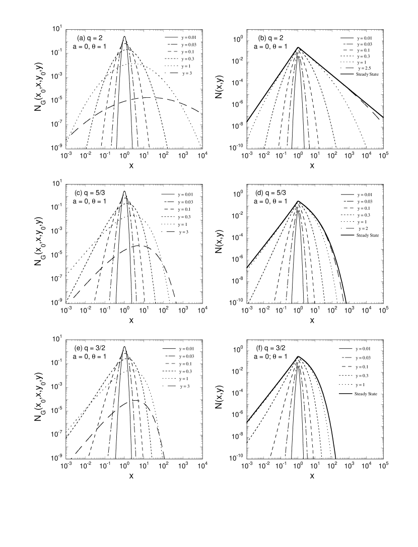
Figure 2: Green’s function solutions to the time-dependent stochastic particle acceleration equation for $x_{0}=1$. The left panels depict the impulsive-injection solution, $N_{{}_{\rm G}}$ (eqs. [46] and [49]), and the right panels illustrate the response to uniform, continuous injection, $N$ (eq. [54]), with $\dot{N}_{0}=D_{*}=1$. Note that $N$ approaches the corresponding steady-state solution (eqs. [56] and [58]) as $y$ increases. The indices of the wave turbulence spectra are indicated, with $q=2$ for hard-sphere scattering, $q=5/3$ for a Kolmogorov cascade, and $q=3/2$ for a Kraichnan cascade.

The panels on the left-hand side of Figure 2 depict the time-dependent Green’s function solution, $N_{{}_{\rm G}}$, describing the evolution of the particle distribution in the plasma resulting from impulsive monoenergetic injection at $y=0$. Results are presented for the hard-sphere scattering case ($q=2$), computed using equation (49), and for the Kolmogorov ($q=5/3$) and Kraichnan ($q=3/2$) cases, evaluated using equation (46). The only acceleration mechanism considered here is the stochastic acceleration associated with the second-order Fermi process, and therefore we set $a=0$. The escape parameter $\theta$ is set equal to unity, so that the timescale for escape is comparable to the diffusion timescale. As the wave turbulence spectrum becomes steeper (i.e., as $q$ increases), a larger fraction of the turbulence energy is contained in waves with long wavelengths, which interact resonantly with higher energy particles. Steeper turbulence spectra therefore produce harder particle distributions, as can be confirmed in the plots. Consequently we conclude that an ensemble of hard sphere scattering centers is more effective at accelerating nonthermal particles compared with a Kolmogorov wave spectrum, which in turn is more effective than a Kraichnan spectrum.

The panels on the right-hand side of Figure 2 illustrate the buildup of the particle spectrum in the plasma, $N(x,y)$, due to continual monoenergetic injection beginning at $y=0$, computed by evaluating numerically the integral in equation (54). We have set $a=0$ and therefore the acceleration is purely stochastic. As $y\to\infty$, the spectrum approaches the steady-state form given by equation (56) for $q<2$ or by equation (58) for $q=2$. In the hard-sphere case ($q=2$), the particle spectrum displays a power-law shape at high energies in agreement with equation (58). However, when $q<2$, particle escape dominates over acceleration at high energies, and therefore the steady-state distribution is truncated, even in the absence of radiative losses. This effect produces the quasi-exponential turnovers exhibited by the stationary spectra when $q=5/3$ and $q=3/2$. Particle escape in these cases mimics energy losses due to, for example, synchrotron emission from electrons.

Figure 3: Evolution of the particle distribution in the plasma resulting from monoenergetic injection with $q=5/3$, $a=0$, $\theta=0.1$, and $x_{0}=1$. Panel (a) depicts the Green’s function, $N_{{}_{\rm G}}$, resulting from impulsive monoenergetic injection (eq. [46]), and panel (b) illustrates the response to continual monoenergetic injection (eq. [54]) and the corresponding steady-state solution (eq. [56]) for $\dot{N}_{0}=D_{*}=1$.

Figures 3 and 4 illustrate the effects of varying the values of the escape parameter $\theta$ and the systematic acceleration/loss parameter $a$ for the $q=5/3$ case. In Figure 3, we set $a=0$ and $\theta=0.1$, which represents a particle escape timescale that is an order of magnitude larger than the corresponding case depicted in Figure 2. The longer escape time allows the particles to be accelerated to higher mean energies before diffusing out of the plasma, and the decay of the particle density at late times takes place much more slowly than for larger values of $\theta$. The hardening of the spectra causes the quasi-exponential cutoffs to move to higher energies, and the same effect can also be noted in the corresponding stationary solutions. The calculations represented in Figure 4 include additional systematic acceleration processes that are modeled by setting $a=2$. The enhanced particle acceleration further hardens the spectrum and shifts the cutoff to even higher energies. Although the slope of the low-energy particle distribution ($x<x_{0}$) is not altered much when only $\theta$ is varied (see Figs. 2 and 3), this slope becomes significantly steeper when $a$ is increased, as indicated in Figure 4.

In the left-hand panels of Figures 5 and 6 we plot the time-dependent solution for the Green’s function describing the escaping particles, $\dot{N}_{{}_{\rm G}}^{\rm esc}$, resulting from impulsive monoenergetic particle injection (eq. [60]) when $q=5/3$. The right-hand panels illustrate the buildup of the escaping spectrum, $\dot{N}^{\rm esc}$ (eq. [64]), resulting from continual injection beginning at $y=0$. Note the transition to the steady-state solution, $\dot{N}_{\rm ss}^{\rm esc}$ (eq. [65]), as $y\to\infty$. In Figure 5 we set $\theta=0.1$ and $a=0$, and in Figure 6 we set $\theta=0.1$ and $a=2$. Included for comparison are the corresponding spectra describing the particle distributions in the plasma at the same values of $y$. We point out that the escaping particle spectra are significantly harder than the in situ distributions, which reflects the preferential escape of the high-energy particles resulting from the momentum dependence of the escape timescale when $q<2$ (see eq. [9]).

Figure 4: Same as Fig. 3, except $a=2$.

5 DISCUSSION AND SUMMARY

We have derived new, closed-form solutions (eqs. [46] and [68]) for the time-dependent Green’s function representing the stochastic acceleration of relativistic ions interacting with MHD waves. The analytical results we have obtained describe the time-dependent distributions for both the accelerated (in situ) and the escaping particles. The Fokker-Planck transport equation considered here includes momentum diffusion with coefficient $D(p)\propto p^{q}$, particle escape with mean timescale $t_{\rm esc}\propto p^{q-2}$, and additional systematic acceleration/losses with a rate proportional to $p^{q-1}$, where $p$ is the particle momentum and $q$ is the index of the wave turbulence spectrum. This specific scenario describes the resonant interaction of particles with fast-mode and Alfvén waves, which is one of the fundamental acceleration processes in high-energy astrophysics (e.g., Dermer et al., 1996).

The new analytical result complements the work of Park & Petrosian (1995) since it is applicable for any $q<2$ provided $s_{\rm pp}=q-2$, where $s_{\rm pp}$ is the power-law index used by these authors to describe the momentum dependence of the escape timescale. The most closely related previous result is given by their equation (59), which treats the case with $q\neq 2$ and $s_{\rm pp}=0$, corresponding to a momentum-independent escape timescale. Our analytical solution (eq. [46]) agrees with theirs in the limit $q\to 2$, as expected. The general features of our new solution were discussed in § 4, where it was demonstrated that increasingly hard particle spectra result from larger values of the wave index $q$, smaller values of the escape parameter $\theta$, and larger values of the systematic acceleration parameter $a$. The rich behavior of the solution as a function of momentum, time, and the parameters $q$, $\theta$, and $a$ provides useful physical insight into the nature of the coupled energetic/spatial particle transport in astrophysical plasmas.

Figure 5: Evolution of the particle distribution resulting from monoenergetic injection with $q=5/3$, $a=0$, $\theta=0.1$, $x_{0}=1$, $\dot{N}_{0}=1$, and $D_{*}=1$. Panel (a) treats the case of impulsive injection, with the thin lines representing the particle distribution in the plasma (eq. [46]) and the heavy lines denoting the escaping particle spectrum (eq. [60]) in units of $\theta$. Panel (b) illustrates the response to continual monoenergetic injection for the particle distribution in the plasma (eqs. [54] and [56]; thin lines) and for the escaping particle spectrum (eqs. [64] and [66]; heavy lines). See the discussion in the text.

Figure 6: Same as Fig. 5, except $a=2$.

The solutions presented here can be used to describe the acceleration and transport of relativistic ions in astrophysical environments in which the turbulence spectrum is very poorly known and can be approximated by a power law, such as $\gamma$-ray bursts, active galaxies, magnetized coronae around black holes, and the intergalactic medium in clusters of galaxies. For example, the hard X-ray emission from black-hole jet sources such as Cygnus X-1 (Malzac et al., 2006) and the microquasar LS 5039 (Aharonian et al., 2005) could be powered by the stochastic acceleration of ions in a black-hole accretion disk corona that subsequently escape and interact with surrounding material. In this scenario, persistent acceleration of monoenergetic particles injected into the corona, or flaring episodes averaged over a sufficiently long time, would produce a time-averaged escaping distribution of relativistic protons given by equation (68) for $q<2$. Assuming only stochastic acceleration, so that $a=0$, the number distribution of escaping particles with $x\geq x_{0}$ takes the form

$$\dot{N}_{\rm ss}^{\rm esc}(x)\propto x^{(7-3q)/2}K_{{\beta-1\over 2}}\left({\sqrt{\theta}x^{2-q}\over 2-q}\right)\propto\cases{x^{3-2q}\ ,&$x\ll\left({2-q\over\sqrt{\theta}}\right)^{1/(2-q)}$\cr x^{(5-2q)/2}\exp\left(-{\sqrt{\theta}x^{2-q}\over 2-q}\right)\ ,&$x\gg\left({2-q\over\sqrt{\theta}}\right)^{1/(2-q)}$\cr}.$$ (70)

When the escaping hadrons collide with ambient gas or stellar wind material, they would generate X-rays and $\gamma$-rays via a pion production cascade with a very hard spectrum leading up to a quasi-exponential cutoff. The Gamma ray Large Area Space Telescope (GLAST) telescope will be able to provide detailed spectra from Galactic black-hole sources and unidentified EGRET $\gamma$-ray sources to test for the existence of this hard component. Our new analytical solution can also be used to model the variability of radiation from ions accelerated in the accretion-disk coronae of Seyfert galaxies by changing the level of turbulence. Flaring $\sim 100\,$MeV – GeV radiation could be weakly detected by GLAST as a consequence of this process. Additional applications of our work include studies of the stochastic acceleration of relativistic cosmic rays in $\gamma$-ray bursts (Dermer & Humi, 2001).

The results we have obtained describe both the momentum distribution of the particles in the plasma, and the momentum distribution of the particles that escape to form energetic outflows. Since the solutions do not include inverse-Compton or synchrotron losses, which are usually important for energetic electrons, they are primarily applicable to cases involving ion acceleration. In order to treat the acceleration of relativistic electrons, a generalized calculation including both stochastic particle acceleration and radiative losses is desirable, and we are currently working to extend the analytical model presented here to incorporate these effects. Beyond the direct utility of the new analytical solutions for probing the nature of particle acceleration in astrophysical sources, we note that they are also useful for benchmarking numerical simulations.

Appendix A APPENDIX

In this section we explore the relationship between the momentum diffusion coefficient $D(p)$ and the mean rate of change of the particle momentum and kinetic energy, using the integral method outlined by Subramanian et al. (1999).

A.1 Mean Rate of Change of Momentum Due to Stochastic Acceleration

In the case of pure stochastic acceleration, the transport equation (1) reduces to

$${\partial f\over\partial t}={1\over p^{2}}{\partial\over\partial p}\left[p^{2}\,D(p)\,{\partial f\over\partial p}\right]\ .$$ (A1)

The mean momentum, $\langle p\rangle$, is defined as a function of $t$ by

$$\langle p\rangle\equiv{1\over n}\int_{0}^{\infty}4\pi p^{3}\,f(p,t)\,dp\ ,$$ (A2)

where the number density $n$ is related to $f$ via equation (2). The associated mean rate of change of the momentum is given by

$$\Big{\langle}{dp\over dt}\Big{\rangle}={1\over n}\int_{0}^{\infty}4\pi p^{3}\,{\partial f\over\partial t}\,dp\ .$$ (A3)

Combining this relation with the transport equation (A1) yields

$$\Big{\langle}{dp\over dt}\Big{\rangle}={1\over n}\int_{0}^{\infty}4\pi p\,{\partial\over\partial p}\left(p^{2}D{\partial f\over\partial p}\right)dp\ .$$ (A4)

Integrating by parts once gives

$$\Big{\langle}{dp\over dt}\Big{\rangle}=-{1\over n}\int_{0}^{\infty}4\pi p^{2}D{\partial f\over\partial p}\,dp\ ,$$ (A5)

and integrating by parts a second time yields

$$\Big{\langle}{dp\over dt}\Big{\rangle}={1\over n}\int_{0}^{\infty}4\pi f{d\over dp}\left(p^{2}D\right)dp\ .$$ (A6)

It is sufficient for our purposes to consider the evolution of the particle distribution $f$ satisfying the monoenergetic initial condition

$$f(p,t)\bigg{|}_{t=t_{0}}=A_{0}\,\delta(p-p_{0})\ .$$ (A7)

Combining this relation with equation (A6), we find that at the initial time $t=t_{0}$,

$$\Big{\langle}{dp\over dt}\Big{\rangle}\Bigg{|}_{t=t_{0}}={1\over p^{2}}{d\over dp}\left(p^{2}D\right)\Bigg{|}_{p=p_{0}}\ .$$ (A8)

Dropping the subscript “0” without loss of generality, we conclude that the mean rate of change of the momentum for particles with momentum $p$ at time $t$ is given by

$$\Big{\langle}{dp\over dt}\Big{\rangle}={1\over p^{2}}{d\over dp}\left(p^{2}D\right)\ ,$$ (A9)

which agrees with equation (7).

A.2 Mean Rate of Change of Kinetic Energy Due to Stochastic Acceleration

The mean kinetic energy, $\langle\epsilon\rangle$, is defined by

$$\langle\epsilon\rangle\equiv{1\over n}\int_{0}^{\infty}4\pi p^{2}\epsilon\,f\,dp\ ,$$ (A10)

where $\epsilon$ is given by equation (3). The associated mean rate of change is given by

$$\Big{\langle}{d\epsilon\over dt}\Big{\rangle}={1\over n}\int_{0}^{\infty}4\pi p^{2}\epsilon\,{\partial f\over\partial t}\,dp\ ,$$ (A11)

which can be combined with the transport equation (A1) to obtain

$$\Big{\langle}{d\epsilon\over dt}\Big{\rangle}={1\over n}\int_{0}^{\infty}4\pi\epsilon\,{\partial\over\partial p}\left(p^{2}D{\partial f\over\partial p}\right)dp\ .$$ (A12)

As in the previous section, we integrate by parts to find that

$$\Big{\langle}{d\epsilon\over dt}\Big{\rangle}=-{1\over n}\int_{0}^{\infty}4\pi{d\epsilon\over dp}\,p^{2}D{\partial f\over\partial p}\,dp\ .$$ (A13)

Next we employ the derivative relation

$${d\epsilon\over dp}=v$$ (A14)

and integrating by parts again to obtain

$$\Big{\langle}{d\epsilon\over dt}\Big{\rangle}={1\over n}\int_{0}^{\infty}4\pi f{d\over dp}\left(vp^{2}D\right)dp\ .$$ (A15)

Applying the initial condition given by equation (A7), we find that at the initial time $t=t_{0}$

$$\Big{\langle}{d\epsilon\over dt}\Big{\rangle}\Bigg{|}_{t=t_{0}}={1\over p^{2}}{d\over dp}\left(vp^{2}D\right)\Bigg{|}_{p=p_{0}}\ .$$ (A16)

Dropping the subscript “0” without loss of generality, we conclude that the mean rate of change of the kinetic energy for particles with momentum $p$ at time $t$ is given by

$$\Big{\langle}{d\epsilon\over dt}\Big{\rangle}={1\over p^{2}}{d\over dp}\left(p^{2}vD\right)\ ,$$ (A17)

which agrees with equation (8) and with equation (13) from Miller & Ramaty (1989).

References

- Abramowitz & Stegun (1970) Abramowitz, M., & Stegun, I. A. 1970, Handbook of Mathematical Functions (New York: Dover)
- Aharonian et al. (2005) Aharonian, F., et al. 2005, Science, 309, 746
- Atoyan & Dermer (2004) Atoyan, A., & Dermer, C. D. 2004, ApJ, 617, L123
- Becker (1992) Becker, P. A. 1992, ApJ, 397, 88
- Becker (2003) Becker, P. A. 2003, MNRAS, 343, 215
- Blandford & Eichler (1987) Blandford, R., & Eichler, D. 1987, Phys. Rep., 154, 1
- Brunetti et al. (2004) Brunetti, G., Blasi, P., Cassano, R., & Gabici, S. 2004, MNRAS, 350, 1174
- Butkov (1968) Butkov, E. 1968, Mathematical Physics (London: Addison-Wesley)
- Dermer & Humi (2001) Dermer, C. D., & Humi, M. 2001, ApJ, 556, 479
- Dermer et al. (1996) Dermer, C. D., Miller, J. A., & Li, H. 1996, ApJ, 456, 106
- Fermi (1949) Fermi, E. 1949, Physical Review, 75, 1169
- Gradshteyn & Ryzhik (1980) Gradshteyn, I. S., & Ryzhik, I. M. 1980 (New York: Academic Press)
- Kirk (1994) Kirk, J. G. 1994, Saas-Fee Advanced Course 24: Plasma Astrophysics, 225
- Liu et al. (2004a) Liu, S., Petrosian, V., & Mason, G. M. 2004a, ApJ, 613, L81
- Liu et al. (2004b) Liu, S., Petrosian, V., & Melia, F. 2004b, ApJ, 611, L101
- Liu et al. (2006) Liu, S., Melia, F., & Petrosian, V. 2006, ApJ, 636, 798
- Malzac et al. (2006) Malzac, J., et al. 2006, A&A, 448, 1125
- Melrose (1974) Melrose, D. B. 1974, Sol. Phys., 37, 353
- Melrose (1980) Melrose, D. B. 1980 (New York: Gordon and Breach)
- Miller & Ramaty (1989) Miller, J. A., & Ramaty, R. 1989, ApJ, 344, 973
- Miller et al. (1990) Miller, J. A., Guessoum, N., & Ramaty, R. 1990, ApJ, 361, 701
- Park & Petrosian (1995) Park, B. T., & Petrosian, V. 1995, ApJ, 446, 699
- Petrosian (2001) Petrosian, V. 2001, ApJ, 557, 560
- Ramaty (1979) Ramaty, R. 1979, AIP Conf. Proc. 56: Particle Acceleration Mechanisms in Astrophysics, eds. J. Arons, C. Max, & C. McKee, 56, 135
- Reif (1965) Reif, F. 1965, Fundamentals of Statistical and Thermal Physics (New York: McGraw-Hill)
- Schlickeiser (1984) Schlickeiser, R. 1984, A&A, 136, 227
- Schlickeiser et al. (1987) Schlickeiser, R., Sievers, A., & Thiemann, H. 1987, A&A, 182, 21
- Schlickeiser (1989a) Schlickeiser, R. 1989a, ApJ, 336, 243
- Schlickeiser (1989b) Schlickeiser, R. 1989b, ApJ, 336, 264
- Schlickeiser & Steinacker (1989) Schlickeiser, R., & Steinacker, J. 1989, Sol. Phys., 122, 29
- Subramanian et al. (1999) Subramanian, P., Becker, P. A., & Kazanas, D. 1999, ApJ, 523, 203
- Tademaru et al. (1971) Tademaru, E., Newman, C. E., & Jones, F. C. 1971, Ap&SS, 10, 453
- Waxman (1995) Waxman, E. 1995, Physical Review Letters, 75, 386
- Zhou & Matthaeus (1990) Zhou, Y., & Matthaeus, W. H. 1990, JGR, 95, 14881