Exploring the spectroscopic diversity of Type Ia Supernovae

Abstract

The velocities and equivalent widths (EWs) of a set of absorption features are measured for a sample of 28 well-observed Type Ia supernovae (SNe Ia) covering a wide range of properties. The values of these quantities at maximum are obtained through interpolation/extrapolation and plotted against the decline rate, and so are various line ratios. The SNe are divided according to their velocity evolution into three classes defined in a previous work of Benetti et al.: low velocity gradient (LVG), high velocity gradient (HVG), and FAINT. It is found that all the LVG SNe have approximately uniform velocites at B maximum, while the FAINT SNe have values that decrease with increasing $\Delta m_{15}(B)$, and the HVG SNe have a large spread. The EWs of the Fe-dominated features are approximately constant in all SNe, while those of intermediate mass element (IME) lines have larger values for intermediate decliners and smaller values for brighter and FAINT SNe. The HVG SNe have stronger Si ii 6355-Å lines, with no correlation with $\Delta m_{15}(B)$. It is also shown that the Si ii 5972 Å EW and three EW ratios, including one analogous to the $\cal R$(Si ii) ratio introduced by Nugent et al., are good spectroscopic indicators of luminosity. The data suggest that all LVG SNe have approximately constant kinetic energy, since burning to IME extends to similar velocities. The FAINT SNe may have somewhat lower energies. The large velocities and EWs of the IME lines of HVG SNe appear correlated with each other, but are not correlated with the presence of high-velocity features in the Ca ii infrared triplet in the earliest spectra for the SNe for which such data exist.

1 Introduction

Understanding the physics of Type Ia Supernova (SN Ia) explosions is one of the most important issues of contemporary astrophysics, given the role SNe Ia play as distance indicators for cosmology and as main producers of heavy elements in the Universe. One of the keys to enter the secrets of SNIa explosions is to study their diversity.

SNe Ia are thought to be the thermonuclear explosion of carbon–oxygen white dwarfs driven to ignition conditions by accretion in a binary system. Since explosive burning of the CO mixture occurs when the white dwarf’s mass is close to the Chandrasekhar limit, it has long been speculated that SNe Ia should be good candidates for standard candles.

While earlier impressions were that SNe Ia are quite homogeneous, it was later noted that there are intrinsic differences among them. However, correlations have been found that describe SNe Ia as a one-parameter family. Phillips (1993) measured the decline in $B$-band magnitude from $B$-band maximum to 15 d later, a quantity he called $\Delta m_{15}(B)$, and found that brighter objects have a smaller decline rate than dimmer ones. The decline rate therefore not only is useful for arranging SNe Ia in a ‘photometric’ one-parameter sequence, but should also reflect, although possibly in a gross way, SN Ia physics.

This is matched by a spectroscopic sequence (Nugent et al., 1995), defined by $\cal R$(Si ii), the ratio of the depth of two absorptions at 5800 and 6100 Å, both of which are usually attributed to Si ii lines. This ratio correlates with the absolute magnitude of SNe Ia and, in turn, with the rate of decline. Spectroscopic models suggest that most spectral differences are due to variations in the effective temperature. In the context of Chandrasekhar-mass explosions, these variations can be interpreted in terms of a variation in the mass of ⁵⁶Ni produced in the explosion. The relative behaviour of the two Si ii lines is, however, counterintuitive, and still lacks a thorough theoretical explanation. Garnavich et al. (2004) suggest that the bluer line is affected by Ti ii lines for objects with $\Delta m_{15}(B)\geq 1.2$, but this is not supported by detailed spectral synthesis studies of SN 1991bg and SN 2002bo (Mazzali et al. 1997; Stehle et al. 2005).

Although a one-parameter description of SNe Ia has proved to be very useful, it does not completely account for the observational diversity of SNe Ia (e.g.  Benetti et al., 2004, 2005). In fact, earlier studies (e.g.  Patat et al., 1996; Hatano et al., 2000) suggest that the photospheric expansion velocity, which can be taken as a proxy for the kinetic energy release in the explosion, correlates with neither $\Delta m_{15}(B)$ nor $\mathcal{R}$(Si ii) [see also Wells et al. (1994) for an early attempt to correlate SNIa observables]. However, Benetti et al. (2005) found a spread in the time-averaged rate of decrease of the expansion velocity of the Si ii 6355-Å absorption after maximum, which might suggest another means of classifying SNe Ia. They used $\langle\dot{v}\rangle$ among other parameters to perform a computer-based hierarchical cluster analysis of a sample of 26 SNe Ia. This led to a partitioning of the SNe into three groups, called, respectively, high velocity gradient (HVG; $\langle\dot{v}\rangle=97\pm 16$ km s${}^{-1}\,$d^-1), low velocity gradient (LVG; $\langle\dot{v}\rangle=37\pm 18$ km s${}^{-1}\,$d^-1), and FAINT. The FAINT group includes SNe that are intrinsically dim, on average $\sim 2$ mag fainter than SNe belonging to the other two groups. Their velocity gradient is large, $\langle\dot{v}\rangle=87\pm 20$ km s${}^{-1}\,$d^-1. HVG and LVG SNe have similar mean absolute blue magnitude at maximum, but the HVG SNe have a smaller spread in $\Delta m_{15}(B)$, and all SNe Ia with $\Delta m_{15}(B)\leq 1.05$ are LVGs. Benetti et al. (2005) confirmed the relation between $\cal R$(Si ii) and $\Delta m_{15}(B)$, but find a larger scatter among LVG SNe, especially at the bright end.

Spectra are an invaluable source of information, on both kinematics and the chemical composition of the ejecta. While other studies aim at extracting information by reproducing spectra or line ratios with models (Stehle et al. 2005; Bongard et al. 2005), this work is based on direct measurements of spectroscopic data, providing therefore a complementary approach [see also Folatelli (2004), who emphasized the time evolution]. We focus on a comparison of the spectral properties of different SNe. This requires a large enough number of objects with spectral data of good quality and at comparable epochs of evolution. During the last few years, the number of such objects has increased tremendously.

This work is thus based upon a collection of published as well as unpublished spectral data for 28 SNe Ia, 25 of which are from Benetti et al. (2005). The expansion velocities of some clearly defined featues were measured systematically and consistently, as were their equivalent widths (EWs, see section 2.2). With the aim of gathering information about the differences in chemical composition, we studied a number of line strength ratios, involving lines of intermediate mass elements (IME) such as S or Si as well as lines of Fe group elements. Thus, our study should explore the extent of nuclear burning in different objects. It also turned out to be interesting to look at ratios involving a line of oxygen as representative of unburned or partially burned material. Taking into account seven different lines, this paper aims to extend the studies cited above.

Measurements were performed for different objects at comparable epochs of evolution, so that values can be contrasted, differences examined and links to the physical properties of the objects identified. One possible approach is to examine the relation between line velocities and strenghts on the one hand and the light curve decline rate on the other.

2 Spectral data and measurements

We used the sample of SNe from Benetti et al. (2005), except for one object (1999cw) for which there was no spectum at a suitable epoch (see below). Three new objects (1991M, 2004eo, 2005bl) were added; the sample was divided into the three groups defined in Benetti et al. (2005). An overview of the objects, group assignment, $\Delta m_{15}(B)$ and $\langle\dot{v}\rangle$ values, and the sources of the respective spectra is given in Table 1. These data are taken from Benetti et al. (2005) – see also references therein – except for additional/updated objects (see table notes), for which they were newly calculated.

For our measurements, we selected from our database about 100 spectra containing at least one absorption that can be clearly identified.

In a SN Ia spectrum near maximum, several such features can be seen; Table 2 lists the lines used for this study. The EW ratios considered are given in Table 3. For an overview of features, see Fig. 1.

Starting from the blue end, a feature typical for SNe Ia shows up around $3750\,$Å  which is due to the Ca ii H&K lines. This feature is, however, not evaluated in this study because the spectra of some objects do not extend far enough to the blue to include that feature.

The first two features evaluated, viewed from the blue, are troughs (i.e. unresolved blends of many lines) mostly related to Fe lines. The bluer one is centered around $\sim 4300\,$Å in the observed spectra, and is made not only of Fe ii and Fe iii  lines, but has also contributions from Mg ii  for the fainter SNe and – for very faint objects – strong Ti ii lines. The other trough is centered around $\sim 4800\,$Å in the spectra and contains lines of Fe ii and Fe iii with almost no contamination by other elements except some Si ii lines. Both features are frequently accompanied by small ‘notches’ at their edges. These are weaker features that are not necessarily caused by Fe lines. The determination of the edges of the troughs is therefore difficult; special care was taken that this was done in a consistent way for all objects. Even then, measurements of the $\sim 4300$-Å trough for the faintest objects cannot be compared with the rest; the appearance of Ti ii lines affects not only the depth of the trough but also its blue extent. Also, measurements for 1991T-like objects should be taken with some care because of the Fe iii lines dominating the feature before maximum light (see Mazzali, Danziger & Turatto 1995).

Lines related to the IME ions S ii and Si ii are perhaps the most characteristic features of SN Ia spectra. S ii absorption causes a W-shaped trough with observed minima at $\sim 5250$ and 5400 Å, respectively. The minima can be attributed to S ii multiplets with their strongest lines at $\sim 5445$ and 5640 Å, respectively. All those transitions originate from relatively high-lying lower levels, which causes a significant weakening of the S ii absorption at low temperatures. Si ii features, on the other hand, can be seen at $\sim 5750$ and 6100 Å. Both features are blends, with average rest wavelength 5972 and 6355 Å, respectively. The redder line is by far the stronger, and its temperature dependence is rather weak. On the other hand, the strength of the 5972-Å absorption is strongly correlated with temperature, but the correlation is opposite to intuitive expectations from atomic physics (see also section 4.4). An explanation might involve the presence of other, weaker lines.

In the spectra of almost all SNe, another feature is visible around $7500$ Å near maximum light, which is a blend of two very close O i lines with a mean rest wavelength of 7773 Å. The absorption is especially prominent in spectra of FAINT SNe. Unfortunately, the feature suffers from contamination by the telluric absorption at $7605$ Å (and sometimes perhaps also by Mg ii lines), which makes measurements complicated (see section 2.2).

All measurements were carried out using iraf (see Acknowledgments). The spectra were deredshifted; $z$ values were taken from wavelength measurements of interstellar Na i D and Ca ii H&K lines, or – if this was uncertain – from either the literature if any was available or from the LEDA or NED catalogues (using galaxy recession velocities). No reddening correction was applied to the spectra. As discussed below, reddening should have negligible impact on the measured values.

The spectral data do not cover the same epochs for all objects. In order to include as many SNe as possible, we interpolated/extrapolated EW and velocity values at $t=0\;\textrm{d}$ for each object by performing a least-squares fit of the measured values at different times (this also yields standard deviations used as statistical error estimates). Since the features can be assumed to evolve linearly in a limited interval of time, we evaluated spectra from –5 to +5 d relative to $B$ maximum. In cases where only one or two spectra were available in this range, additional spectra from epochs between –8 and +6.5 d were used if available (for measurements of the Si ii $\lambda 5972$ EW and velocity, and of the S ii EW, the upper limit was +5 d in all cases, as these values evolve rapidly at later times for some objects).

After this selection, some objects remained with only one or two spectra available; this required a special evaluation procedure. In cases with two spectra, the error cannot be computed from the regression; it was therefore calculated by propagating the errors of the single measurements instead. In cases with only one spectrum, the value from this spectrum is given in the diagrams, if it can be expected that the evolution between the date of $B$ maximum and that of the spectrum is not too rapid. The error was then calculated by adding to the error of measurement (see below) an estimate for the error in the estimated time. The latter was computed as the average slope of the regression lines for objects belonging to the same SN group (with $\geq 3$ spectra available), multiplied by the time offset of the single spectrum relative to the day of $B$ maximum.

For the SNe 1984A and 2002dj EW measurements, the described procedure is not reasonable, as the spectral coverage is sparse around $B$ maximum, and the observations of these two objects show a particularly pronounced non-linear time evolution for many EWs. The EW values and respective uncertainties were thus obtained by performing a quadratic polynomial fit to all available data between –10 and +10 d relative to $B$ maximum.

Ratios were calculated from the $EW(t=0)$ values obtained as described; the errors attached to the ratios were computed by propagating the errors of the EWs quadratically.

2.1 Velocity measurements

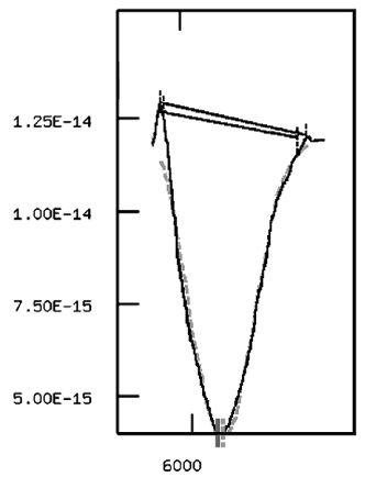
Figure 2: Examples for measurements: pseudo-continua are marked in black; a gaussian fit and its centroid in light grey (dashed). A manual centroid estimate is marked in dark grey.

The mean expansion velocity of a given line was determined from the blueshift of the absorption relative to the rest wavelength. The velocity thus derived is physically meaningful only for single lines or for close multiplets that are sufficiently isolated from other strong features. Since most lines have a P Cygni shape and are blends, one has to think thoroughly about how to measure the ‘mean’ wavelength of an absorption. We used two different methods: The first is to use the gaussian fit routine within iraf; the second is to estimate the centre of the absorption by eye (taking into account problems such as the sloping continuum). The values obtained from several such measurements were then averaged; the respective standard deviation is a crude estimate of the error introduced by the manual measurements, and was used to calculate the error in the cases mentioned above. Fig. 2 shows an example of how measurements were performed.

2.2 Equivalent width measurements

As a measure of line strength, we take the equivalent width (EW). This is defined as:

$$EW=\int^{\lambda_{1}}_{\lambda_{2}}\frac{F_{\rm C}(\lambda)-F(\lambda)}{F_{\rm C}(\lambda)}d\lambda,$$ (1)

where $F(\lambda)$ is the flux density level in the spectrum and $F_{\rm C}(\lambda)$ the continuum flux density. EW is insensitive to multiplication of the flux density spectrum by a constant between $\lambda_{1}$ and $\lambda_{2}$. Therefore, if $\lambda_{1}$ and $\lambda_{2}$ are not too far away from each other, reddening effects can be neglected. Other ‘multiplicative errors’ are also suppressed.

The EW of an absorption (or an emission) line can be measured inside iraf (when showing spectra by splot) by entering the beginning and ending wavelengths of the line, as well as the continuum level at those wavelengths. The main difficulty is to define the continuum and the starting and ending points for a feature, especially considering that the lines have P Cygni profiles. We proceeded as follows (see Fig. 2):

Since a ‘real’ continuum level cannot be determined in SN Ia spectra owing to the multitude of line absorptions, for a single P Cygni profile we defined a pseudo-continuum level to be the flux density level near the edges of the feature, neglecting the influence the emission component has on this. The edges of a feature were set roughly where the slope of the flux curve equals the slope of an imaginary pseudo-continuum curve joining the opposite sides of the line. The error involved with this procedure has no effect on the comparative study as long as all measurements are done consistently. Some lines and absorption troughs regularly have poorly determinable or jagged edges. In these cases, care was taken that the measurements were done as homogeneously as possible for all objects.

EW measurements were carried out several times (see Fig. 2), taking into account reasonable upper and lower estimates of the continuum level and the starting and ending points. The standard deviations thereby obtained for the EW values is again a rough estimate of the errors introduced by the manual input of beginning/ending points and the continuum level, and was further evaluated in the above-mentioned cases.

The O i $\lambda 7773$ line requires special attention. In most spectra, it is contaminated by an atmospheric absorption that is not completely removed in the reduction process. In these cases, the atmospheric absorption or its residuals were cut by visual judgement before measuring the EW, and the measurements were carried out eliminating the contamination in different ways, so that the resulting standard deviation roughly represents the error introduced by the snipping process.

3 Expansion velocities

We only measured the velocities of features that comply with the requirements above, namely features that are due to a single ion, since single lines are not available. The lines discussed below are Si ii $\lambda 5972,6355$, and S ii $\lambda 5640$. Measured values are listed in table 4.

3.1 Si ii $\lambda 6355$

The velocities at maximum derived from this line show a big scatter especially at lower $\Delta m_{15}$ values (Fig. 3). However, once the SNe are divided into velocity gradient groups, it turns out that most SNe, covering a wide range of $\Delta m_{15}$, from 0.9 to $\sim 1.7$, and including all LVG, some HVG, and the brightest among the FAINT SNe, have a roughly constant $v$(Si ii $\lambda 6355$), with only a small scatter ($11000\pm 1000$ km s^-1). HVG objects have a wide range of $v$(Si ii $\lambda 6355$) values, with no correlation with $\Delta m_{15}$, and are responsible for most of the scatter. For FAINT SNe, $v$(Si ii $\lambda 6355$) goes from values comparable to those of the LVG group at $\Delta m_{15}\sim 1.5$–$1.7$ to smaller values as $\Delta m_{15}$ increases.

3.2 Si ii $\lambda 5972$

Although the velocities of this line (Fig. 4) show the same overall tendencies as those derived from the $\lambda 6355$ feature, there are differences especially among the HVG objects. They reach lower maximum velocities, leading to a smaller spread inside this group. A slight tendency to lower values (by $\sim 500$ km s^-1) can also be noted in every group. This is probably due to the fact that the line is weaker and thus forms deeper than Si ii $\lambda 6355$. The apparently larger scatter among LVG objects may be due to the fact that the weak feature often shows a more complicated shape and suffers from noise, making measurements of the centroid less reliable. Also, contamination from other lines may occur.

3.3 S ii $\lambda 5640$

This S ii absorption (Fig. 5) has a behaviour similar to that of the Si ii absorptions discussed above. However, it shows significantly lover velocities than the Si ii $\lambda 6355$ feature, as can be expected since the line is much weaker (see also Blondin et al., 2006). The mean differences from the values derived from the Si ii line for the respective groups are as follows: HVG: $\sim 1000$–$4000$ km s^-1; LVG: $\sim 1000$ km s^-1; FAINT: $\sim 2000$ km s^-1. The spread of values for the HVGs is much smaller in $v$(S ii) than in $v$(Si ii $\lambda 6355$), and also slightly smaller than that of $v$(Si ii $\lambda 5972$).

4 Equivalent widths

In this section, the measurements of the individual features are presented and discussed. Values are given in table 5.

4.1 Fe-Mg(-Ti) trough $\sim 4300$ Å

The EW of this feature is roughly constant for all SNe with $\Delta m_{15}\lesssim 1.8$ (Fig. 6). The lack of evolution suggests that Fe dominates this feature, or at least that the relative contribution of Fe and Mg does not evolve with $\Delta m_{15}$ in the range from 1 to 1.8. HVGs tend to have larger EWs than LVGs because in general they have broader and deeper lines. The EW rapidly increases for FAINT SNe, which is the effect of Ti ii lines becoming very strong in those coolest objects, as was the case for, e.g. , SN 1991bg (Mazzali et al., 1995).

4.2 Fe trough $\sim 4800$

The EW of this feature is essentially constant in all SNe, with a rather large dispersion among objects with the same decline rate (Fig. 7). There is a slight trend to increasing values for the fainter SNe, possibly an effect of the lower temperature which makes the Fe ii lines stronger. On the other hand, some of the peculiar bright SNe, such as SN 1991T, where the Fe iii/Fe ii ratio is large (Mazzali et al. 1995), have values comparable to other SNe, suggesting that Fe iii dominates this feature, as well as the Fe $\sim 4300$ trough, in all LVGs. HVG SNe have again larger values than LVGs, and now the trend is even clearer. Analogy with the FAINT SNe may suggest that the HVG SNe have a lower temperature as a consequence of the higher velocity, but it may also just imply that Fe reaches higher velocities in HVGs, as do S and Si.

SNe 1984A and 1983G have somewhat larger values than the other SNe. This is probably due to the broad-lined nature of these SNe, the SNe Ia with the highest velocities ever recorded (Benetti et al., 2005). The other high-velocity SN, SN 1997bp, could not be measured since its spectra do not extend to the blue.

There is an apparent tendency for SNe to cluster in several small groups. We refrain from interpreting this as an indication of different modes of the explosion, and defer this to a time when more data are available.

4.3 S ii trough $\lambda\sim 5454,\sim 5640$

The EW of the S ii feature (Fig. 8) shows a kind of parabolic trend, with very small scatter. It has a small value for SNe with $\Delta m_{15}<1.0$. It reaches a broad maximum in all other LVG and most HVG SNe with $\Delta m_{15}(B)$$\;=1.1$–$1.5$, and then it progressively declines at $\Delta m_{15}>1.6$. The observed drop may be explained as an effect of the insufficient population of the highly excited lower levels of these lines as the temperatures of the SNe drop. However, at the highest temperatures a reduction in the IME abundance is also required to reproduce the observed weakening of the lines in objects such as SN 1991T (Mazzali et al. 1995). Therefore, it is possible that a trend of increasing abundance going from the slowest to the intermediate decliners, and then decreasing abundance from there to the fastest decliners is also present. The HVG SNe have a slightly larger value than the LVGs, and SN 1984A again stands out by having an anomalously large value.

4.4 Si ii $\lambda 5972$

The EW of the weaker Si ii line (Fig. 9) correlates very well with $\Delta m_{15}$, and could therefore be used as a luminosity indicator just as well as the line strength ratios presented below. This behaviour is at the basis of the observed relation between $\mathcal{R}$(Si ii) and SN luminosity (Nugent et al., 1995), as is illustrated by a plot of $\mathcal{R}$(Si ii) versus EW(Si ii $\lambda 5972$) (Fig. 10) and by the weaker correlation of EW(Si ii $\lambda 6355$) with $\Delta m_{15}$ (see Fig. 11). The very existence of the trend is puzzling, since the Si ii $\lambda 5972$ line originates from a rather highly excited level, and its strength may be expected to correlate with temperature directly rather than inversely. The explanation may involve the contribution of lines from other elements and may require full non-local thermodynamic equilibrium (NLTE) analysis. HVG SNe now blend in with the LVG SNe. This is somewhat surprising, since HVG SNe have the highest velocities (Fig. 3). Clearly, the line does not become more intense in SNe where it gets faster.

4.5 Si ii $\lambda 6355$

This line shows a number of interesting trends (Fig. 11). For most LVGs (with $\Delta m_{15}<1.6$) the EW has a tendency to increase slowly with increasing $\Delta m_{15}$. At larger decline rates, where the FAINT SNe are, the value drops again. The two bright and peculiar LVG SNe, 1991T and 1997br, have much smaller values. This general behaviour is similar to that of the S ii feature, and may be understood as the effect of temperature and possibly of abundance: in SNe 1991T and 1999br the degree of ionisation is higher than in spectroscopically normal objects, and the Si ii line is accordingly weaker, but a low abundance of the IME is also required to reproduce the observed spectra (Mazzali et al. 1995). The Si ii line is strongest for intermediate decliners, where temperature reaches the optimal value for this line and IME abundance possibly reaches a peak. The line weakens in FAINT SNe, which are cooler and possibly have a smaller IME abundance. This effect is less marked than it is in the S ii feature, since the Si ii $\lambda 6355$ originates from levels with a much smaller excitation potential and is less sensitive to temperature. The observed drop may therefore more directly reflect a change in the abundance of Si in near-photospheric mass layers $(\sim 10000\,$km s^-1) of FAINT SNe.

The behaviour of the HVG SNe, on the other hand, is extremely different: these SNe are located almost vertically on the plot: although they cover a smaller range of $\Delta m_{15}$ values than the LVG SNe (1.05 – 1.5 versus 0.9 – 1.5), their EW(Si ii $\lambda 6355$) spans about a factor of two in value. This may reflect the presence of high-velocity absorption in the Si ii line (Mazzali et al., 2005a). SN 1984A is again the most extreme object, followed by SNe 1997bp and 1983G, but these objects appear to be the tip of a smooth distribution. The distribution of HVGs in EW is similar to that in $v$(Si ii $\lambda 6355$) (Fig. 3). Faster lines tend to be broader and deeper. Understanding this kind of behaviour may prove to be a very important step in our effort to understand the systematics of SNe Ia.

4.6 O i $\lambda 7773$

The EW of this line (Fig. 12) tends to rise towards higher $\Delta m_{15}$, but shows quite a big scatter, especially at the bright end. Here, there are both objects which show a very weak O i feature around $B$ maximum as well as objects exhibiting values $\gtrsim 90\,\textrm{\AA}$. Note that these differences can be found both within the HVG and LVG groups, which cover roughly the same range of measured O i EW values. They may partly be due to the above-mentioned difficulties of measuring the O i line. The overall trend of higher values for fainter objects is probably a temperature effect, but it may also reflect changes in abundance. Among FAINT SNe, the trend appears to be reversed. This is possibly due to the decrease of photospheric velocities at the faint end.

5 Line strength ratios

In this section we discuss selected ratios of EW. We focus on ratios that are useful indicators of $\Delta m_{15}$, and on ratios that bear particular physical significance because they involve elements that are synthesised in different parts of the exploding white dwarf. The discussed ratio values are given in table 6.

5.1 $\mathfrak{R}$(Si ii) (Si ii $\lambda 5972$ versus Si ii $\lambda 6355$)

Our measurement is similar to the $\mathcal{R}$(Si ii) value of Nugent et al. (1995), but it differs from it since we use the EW. The EW ratio of the two Si ii lines follows the trend found by Nugent et al. (1995) of increasing $\mathcal{R}$(Si II) with increasing $\Delta m_{15}$ (Fig. 13). However, as noted in Benetti et al. (2005), the scatter at the bright end is larger. As we noted above, the observed behaviour is mainly caused by the unexplained linear increase of the Si ii $\lambda 5972$ line strength for increasing $\Delta m_{15}$.

5.2 Fe-Mg(-Ti) trough $\sim 4300$ versus Fe trough $\sim 4800$

The ratio of the EWs of these two broad absorption troughs (Fig. 14) is fairly constant for $\Delta m_{15}\leq 1.8$. Some of the FAINT SNe (1991bg, 1999by, and 2005bl) have much larger values. The rise at the faint end is clearly due to the appearance of Ti ii lines in the 4300-Å feature at low temperature.

5.3 S ii $\lambda\sim 5454,\sim 5640$ versus Si ii $\lambda 6355$

This value correlates very well with $\Delta m_{15}$ for FAINT objects (Fig. 15). The LVG SNe also correlate reasonably well with $\Delta m_{15}$, with a scatter of $\sim 10$ per cent, but the HVG SNe do not. The average values of the HVG and the LVG group are very different. The HVG SNe show again an almost vertical behaviour, as they did in both the $v$(Si ii $\lambda 6355$) and the EW(Si ii $\lambda 6355$) plot. Since EW(Si ii $\lambda 6355$) is affected, the ratio is smaller for these SNe. For fainter objects, the behaviour mainly seems to reflect the above-mentioned (see section 4.3) changes of ionization structure with decreasing temperature: the S ii line strength decreases rapidly as $\Delta m_{15}$ increases, which is not as much the case for the Si line.

5.4 $\mathfrak{R}$(S,Si) (S ii $\lambda\sim 5454,\sim 5640$ versus Si ii $\lambda 5972$)

This ratio correlates well with $\Delta m_{15}$ for almost all objects, regardless of their group (Fig. 16). It decreases almost linearly with increasing $\Delta m_{15}$, and is thus as suitable as $\mathfrak{R}$(Si ii) as a spectroscopic luminosity indicator. The trend for a smaller ratio with increasing $\Delta m_{15}$ was already present in the previous ‘S/Si’ ratio, but here the scatter is much reduced and both LVG and HVG objects follow the correlation, the differences between the two groups being apparently suppressed. These weaker lines are in fact less affected than Si ii $\lambda 6355$ by the high velocities and the ensuing increased strength, as shown in the EW plots (Fig. 8 and 9). Even SN 1984A follows the general trend: once ratios are taken its large EW values cancel out. We cannot, however, draw any conclusions about Si distribution, velocities, etc. from measurements involving the Si ii$\,\lambda 5972$ feature, because the behaviour of this line is not well understood, as discussed above.

5.5 Si ii $\lambda 6355$ versus Fe trough $\sim 4800$

The plot of this ratio (see Fig. 17) is very interesting, as is its possible meaning, which is discussed below. The ratio exhibits a ‘quadratic’ behaviour: The values are small at small $\Delta m_{15}$, they increase until they reach a peak at $\Delta m_{15}\sim 1.1$–$1.5$ and then they drop again for very faint SNe such as 1991bg, 1997cn and 1999by. The behaviour reflects that of EW(Si ii $\lambda 6355$) but is highly enhanced, suggesting that we are seeing more than just the effect of temperature. The HVG SNe blend in with the other SNe, although they have larger values of both EW(Si ii $\lambda 6355$) and EW(Fe $\sim 4800$).

5.6 S ii $\lambda\sim 5454,\sim 5640$ versus Fe trough $\sim 4800$

This ratio behaves like the previous one (Fig. 18), as could be expected since both Si and S are IME. The FAINT SNe now reach very small values, presumably because of the higher temperature sensitivity of the S ii feature than the Si ii $\lambda 6355$ line.

It is tempting to interpret the behaviour of this ratio and the one above as due not only to temperature, but also to a trend for the brightest SNe to have a higher abundance of Fe relative to IME in layers near the photosphere at maximum ($v\sim 10000$ km s^-1). This is plausible since Fe ii and Si ii have similar ionisation potentials, and should respond similarly to changes in temperature. The observed behaviour may indicate that bright SNe burn more to nuclear statistical equilibrium (NSE) ($\sim 20$ per cent of ⁵⁶Ni has decayed to ⁵⁶Fe at the time of maximum). The drop of the ratio at the largest $\Delta m_{15}$ values may then be due to the fact that now the IME abundance is beginning to decrease in the mass layers near $v_{\mathrm{ph}}$, after reaching a peak at $\Delta m_{15}\sim 1.1$–$1.5$.

Note that $v_{\mathrm{ph}}$ is smaller at larger $\Delta m_{15}$. This implies a lower opacity, which in turn could be associated with a smaller Fe-group abundance relative to IME in the layers between 9000 and 11000 km s^-1, that is between the photosphere of FAINT SNe and that of the other objects. This would suggest that the FAINT SNe produce less NSE material, as is expected both from their dimness and their narrow light curves. The difference between FAINT SNe and brighter ones would be in the degree of burning to NSE at velocities $\sim 10000$ km s^-1, as hypothesised in various models (e.g.  Iwamoto et al., 1999). Burning to IME may also extend to lower velocities in FAINT SNe than in brighter ones.

5.7 $\mathfrak{R}$(Si,Fe) (Si ii $\lambda 5972$ versus Fe trough $\sim 4800$)

This ratio, unlike the previous one, shows an almost constantly rising trend. Over a large range of $\Delta m_{15}$ values, it increases almost linearly with $\Delta m_{15}$ (Fig. 19). This ratio is suitable as a luminosity indicator.

As for a possible explanation of the observed trend, it appears that the ratio is driven by the increasing strength of the Si ii feature with increasing $\Delta m_{15}$, which is not explained as discussed above.

5.8 O i $\lambda 7773$ versus Si ii $\lambda 6355$

This ratio was calculated in order to investigate the relation between O and IME abundance. As we showed above, both EW(Si ii $\lambda 6355$) and EW(S ii) decrease at $\Delta m_{15}>1.5$. If this implies less burning even to IME in the faintest SNe, we might expect O/IME ratios to increase in those objects.

The ratio of O i $\lambda 7773$ and Si ii $\lambda 6355$ shows indeed a slight trend to rise with $\Delta m_{15}$ (Fig. 20), but this is superimposed by a large spread in values of $\gtrsim 25$ per cent at almost every $\Delta m_{15}$ value. Note again that the difficulty in measuring the O i line may affect our results.

5.9 O i $\lambda 7773$ versus S ii $\lambda\sim 5454,\sim 5640$

The S ii line tracks the photosphere more accurately than Si ii $\lambda 6355$. This ratio shows tendency to increase with increasing $\Delta m_{15}$ (Fig. 21), which is enhanced for $\Delta m_{15}\gtrsim 1.5$. While the decrease in S ii line strength for large $\Delta m_{15}$ (Fig. 7) certainly drives the latter trend, and the rise in O i EW causes the tendency for $\Delta m_{15}\lesssim 1.5$, how much all of this is due to decreasing IME abundance compared to oxygen is unclear.

5.10 O i $\lambda 7773$ versus Fe trough $\sim 4800$

This ratio – though exhibiting significant scatter especially at low $\Delta m_{15}$ – shows a clear trend to increase for $\Delta m_{15}\lesssim 1.5$ (Fig. 22). This can be understood by considering the tendency of the O i EW to rise and the behaviour of the Fe $\sim 4800$ trough EW, which is essentially flat. Interestingly, for the faintest objects, an almost linear drop can be observed.

6 Discussion

In this section we briefly discuss the possible implications of the various measurements.

6.1 Photospheric velocities

Near maximum, all LVG, some HVG and some FAINT SNe have a very similar Si ii velocity, $\sim 11000$ km s^-1 (Fig. 3). This can be taken to imply that there is significant nuclear burning (at least to IME) in all these objects, irrespective of their brightness. As we know, $\Delta m_{15}$ depends mostly on the amount of NSE material synthesised (Mazzali et al., 2001, and references therein), while the kinetic energy (KE) depends also on burning to IME (Gamezo, Khokhlov & Oran, 2005). Therefore, all LVG SNe may have a similar KE. The faintest SNe have a lower $v$(Si ii$\lambda 6355$), $\sim 9000$–$10000$ km s^-1. This suggests that there may be less total burning, not just less burning to NSE, and thus possibly less KE, in these SNe.

As for HVG SNe, it is interesting to check whether the observed high velocity is related to the presence of high-velocity features (HVFs, Mazzali et al., 2005b). These are high-velocity absorptions observed mostly in the Ca ii IR triplet in the spectra of almost all SNe Ia earlier than 1 week before maximum. The high velocities measured for HVGs here may be the result of blending of Si ii and S ii HVFs with the lower velocity photospheric lines. Indeed, Si ii HVFs are inferred at earlier times in several SNe, but never seen detached from the main, photospheric component (Mazzali et al., 2005a). Interestingly, no correlation between pre-maximum HVFs and IME velocity at maximum is found: the six SNe that are common to this study and Mazzali et al. (2005b) divide evenly among the HVG (SNe 2002bo, 2002dj, 2002er) and LVG (SNe 2001el, 2003du, 2003kf) groups. Furthermore, while all these SNe have prominent HVFs in the Ca ii IR triplet about one week before maximum or earlier, it is actually the LVG SNe among them that retain strong Ca ii HVFs at about maximum (Mazzali et al., 2005b, Table 3).

It is reasonable to expect that detached HVFs should behave similarly, whether they occur in Ca ii or Si ii (or S ii). Therefore, the rapid decrease of the HVF strength in HVGs may be behind the rapid drop in the Si ii velocity, if Si ii HVFs are not resolved. However, this leaves us with an apparent contradiction: on the one hand, the LVG SNe have the longer-lasting HVFs , but on the other the HVG SNe still have the highest Si ii velocities at maximum. Taken individually, both of these behaviours could be understood in the frame of a scenario where HVFs determine the line velocities, but the fact that they occur together is difficult to accommodate. HVFs may be due to asymmetries in the ejection, or to interaction with circumstellar material, while the velocity at maximum more likely reflects global properties of the explosion.

The S ii velocity behaves like the Si ii velocity (Fig. 5). This line is weaker than the Si ii line, and therefore it is a better tracer of the photosphere. The S ii velocity plot shows that the photosphere moves to progressively lower velocities for increasing $\Delta m_{15}$. This is again to be expected, since $v_{\mathrm{ph}}$ depends on both density and opacity. While the density may be the same, the temperature is lower in fainter SNe, so $v_{\mathrm{ph}}$ may also be lower. The presence of S at $v\sim 7000$ km s^-1 confirms that the ⁵⁶Ni production is small in the faster decliners. Small values for the faintest SNe may also suggest a possibly smaller KE, or even a smaller mass. As for HVGs, they may again be affected by line broadening, although clear S ii HVFs have never been observed. The effect is indeed smaller than seen in the Si ii line, but the riddle mentioned above still stands.

6.2 Spectroscopic luminosity indicators

Besides $\mathfrak{R}$(Si ii), two other line strength ratios correlate particularly well with $\Delta m_{15}$: S ii versus Si ii $\lambda 5972$ [$\mathfrak{R}$(S,Si), Fig. 16] and Si ii $\lambda 5972$ versus Fe $\sim 4800$ [$\mathfrak{R}$(Si,Fe), Fig. 19]. All correlations involve the mysterious Si ii $\lambda 5972$ line, whose EW is at least as well – if not better – correlated with $\Delta m_{15}$ than the ratios, especially at high values of $\Delta m_{15}$. Parameters of least square fits for the respective functions $\Delta m_{15}(\mathrm{ratio}|\mathrm{EW})$ can be found in Table 7; the regression lines are also shown in the respective diagrams. These linear regressions have been calculated over the whole SN Ia variety and not only over normal SN Ia as in Bongard et al. (2005).

6.3 IME ratio differences between HVG and LVG objects

The main difference between HVG and LVG objects, leading to the separation in a hyerarchical cluster analysis, is the velocity development of the Si ii $\lambda 6355$ line after maximum. The parameter $\langle\dot{v}\rangle$ seems to be related to the diversity of SNe Ia beyond the differences described by $\Delta m_{15}$. HVG objects with the same $\Delta m_{15}$ exhibit a wide range of IME velocities (Figs 3 and 5), EW(Si ii $\lambda 6355$) (Fig. 11), and of the ratio EW(S ii) versus EW(Si ii $\lambda 6355$) (Fig. 15). While the spread of velocities could be explained by the presence of IME at different depths in HVGs, the variation in the ratio EW(S ii)/EW(Si ii $\lambda 6355$) is due to the fact that only the Si ii $\lambda 6355$ line has a wide range of EW for the HVG SNe.

6.4 Fe and O versus IME line strength ratios

The line strengths around maximum give the following picture (Si conclusions are always derived from the Si ii $\lambda 6355$ line, as mentioned above): brighter objects tend to contain less oxygen at the velocities probed by the spectra near maximum (Fig. 12). Intermediate decliners contain more silicon and less Fe than slow decliners (Fig. 17). Thus, the photosphere at maximum is deeper in the Fe layer for the slow decliners, while it still inside the Si layer for the intermediate decliners. However, $v_{\mathrm{ph}}$ for these two groups is practically the same, at least within LVG objects, as shown by the $v$(Si) and $v$(S) plots (Fig. 3 and 5). This implies that burning to NSE extends to outer layers in the slow decliners. Very faint objects contain more unburned or partially burned material (i.e. oxygen), probably at the expense of IME (see also Höflich et al., 2002). This is suggested not only by the ratio EW(O i $\lambda 7773$)/EW(S ii) (Fig. 21), but also by the decline of the equivalent widths of the Si ii and S ii lines (Figs 11 and 8). Since the photosphere, as traced by the S ii line, is deeper as $\Delta m_{15}$ increases, this may suggest that the faster decliners have less overall burning.

7 Conclusions

We have systematically measured the velocities and EW of a number of spectral features in SNe Ia around maximum. The SNe have been grouped according to their velocity gradient (Benetti et al., 2005), and we examined different EW ratios searching for systematic trends and for possible hints to the general character of SN Ia explosions. Our results can be summarised as follows.

The photospheric velocity, as indicated by Si ii and S ii lines, is approximately constant for all LVG SNe with $\Delta m_{15}<1.6$. The value declines at larger $\Delta m_{15}$. HVG SNe are found in a limited range of $\Delta m_{15}$, but their velocities are highly variable.

The EW of the Fe-dominated features are approximately constant for all SNe. Those of IME lines are highest for $\Delta m_{15}\approx 1.1$–$1.5$ and are smaller for the brightest and the faintest SNe. HVG SNe have on average larger values, in particular for Si ii $\lambda 6355$. The O i $\lambda 7773$ line is particularly strong in the fainter SNe, and tends to get weaker with increasing luminosity.

Three EW ratios are good indicators of $\Delta m_{15}$: $\mathfrak{R}($Si ii$)$ [EW(Si ii $\lambda 5972$)/EW(Si ii $\lambda 6355$), similar to $\mathcal{R}$(Si ii) in Nugent et al. (1995)], $\mathfrak{R}(\mathrm{Si,S})$ [EW(Si ii $\lambda 5972$)/EW(S ii)], $\mathfrak{R}(\mathrm{Fe,Si})$ [EW(Si ii $\lambda 5972$)/EW(Fe trough $\sim 4800$)]. All three ratios are driven by the EW of the Si ii $\lambda 5972$ line, which itself might thus be the best spectroscopic luminosity indicator. Its behaviour and identification are, however, not well understood; these relations are therefore only empirical.

The ratios of EW(Si ii $\lambda 6355$) and EW(S ii) to EW(Fe trough $\sim 4800$) (Fig. 17 and 18) show a parabolic behaviour: they are small at small $\Delta m_{15}$, reach a peak at $\Delta m_{15}\approx 1.1$–$1.5$, and then decline. While for the S ii line part of this behaviour could be explained as the effect of increasing temperature, the Si/Fe trend may reflect an abundance change. The brightest SNe have more Fe near the maximum-light photosphere ($\sim 10000$ km s^-1). Intermediate decliners have more IME and less Fe at a similar velocity. Faint SNe have a deeper photosphere, indicating both less ⁵⁶Ni and Fe-group elements, and also less IME, suggesting that burning was overall reduced. This is apprently confirmed by high O i EW values for faint SNe.

HVG SNe have the fastest and strongest IME lines. This is, however, not correlated with the presence of Ca ii HVFs. Actually, SNe with the strongest, longer lasting Ca ii HVFs are LVGs. Longer lasting HVFs may slow down the velocity decline, but this does not explain why among the SNe with HVFs the LVG SNe have the lower velocities.

Our results are based on empirical measurements. It would be important to test their implications using models. This is made complicated by the uncertainties in the details of the abundance and density distributions, which can affect model results. We will attempt to do this in a future work.

Table 1: Objects and sources of respective spectra.

SN	$\Delta m_{15}(B)^{\rm a}$	$\langle\dot{v}\rangle\left[\mathrm{km}\,\mathrm{s}^{-1}\,\mathrm{d}^{-1}\right]^{\rm a}$	References for spectra
LVG
89B	$1.34\pm 0.07$	$66\pm 5$	Barbon et al. (1990); Wells et al. (1994)
90N	$1.08\pm 0.05$	$41\pm 5$	Leibundgut et al. (1991); Mazzali et al. (1993)
91T	$0.95\pm 0.05$	$11\pm 5$	Filippenko et al. (1992); Phillips et al. (1992); Ruiz-Lapuente et al. (1992)
92A	$1.47\pm 0.05$	$45\pm 5^{\rm b}$	Asiago archive; Kirshner et al. (1993)
94D	$1.32\pm 0.05$	$39\pm 5$	Patat et al. (1996)
96X	$1.25\pm 0.05$	$46\pm 5$	Salvo et al. (2001)
97br	$1.04\pm 0.15$	$25\pm 5$	Asiago archive; Li et al. (1999)
98bu	$1.04\pm 0.05$	$10\pm 5$	Asiago archive; Jha et al. (1999); Hernandez et al. (2000)
99ee	$0.94\pm 0.04$	$42\pm 5$	Hamuy et al. (2002)
01el	$1.15\pm 0.04$	$31\pm 5$	Wang et al. (2003); Mattila et al. (2005)
03du	$1.06\pm 0.06^{\rm c}$	$31\pm 5$	Stanishev et al. (2006), in preparation
03kf	$1.01\pm 0.05^{\rm c}$	$50\pm 5$	Salvo et al. (2006), in preparation
04eo	$1.46\pm 0.04^{\rm c}$	$45\pm 4$	Pastorello et al. (2006), in preparation
HVG
81B	$1.11\pm 0.07$	$76\pm 7$	Branch et al. (1983)
83G	$1.37\pm 0.10$	$125\pm 20$	H83; M84; Benetti et al. (1991); McDonald archive
84A	$1.21\pm 0.10$	$92\pm 10$	Barbon, Rosino & Iijima (1989)
89A	$1.06\pm 0.10$	$90\pm 10$	Benetti et al. (1991)
91M	$1.51\pm 0.10^{\rm d}$	$92\pm 5$	Asiago archive; Gómez et al. (1996)
97bp	$1.09\pm 0.10$	$106\pm 7$	Asiago archive
02bo	$1.17\pm 0.05$	$110\pm 7$	Benetti et al. (2004)
02dj	$1.12\pm 0.05^{\rm c}$	$86\pm 6$	Pignata et al. (2006), in preparation
02er	$1.33\pm 0.04$	$92\pm 5$	Kotak et al. (2005)
FAINT
86G	$1.78\pm 0.07$	$64\pm 5$	Cristiani et al. (1992)
91bg	$1.93\pm 0.10$	$104\pm 7$	Turatto et al. (1996); Gómez et al. (1996)
93H	$1.70\pm 0.10$	$73\pm 8$	Asiago archive; CTIO Archive
97cn	$1.86\pm 0.10$	$83\pm 10$	Turatto et al. (1998)
99by	$1.87\pm 0.10$	$110\pm 10$	Garnavich et al. (2004)
05bl	$\sim 1.8^{\rm e}$	$73\pm 10$	RTN, in preparation

^a Values from Benetti et al. (2005) unless otherwise stated. $\Delta m_{15}(B)$ values are reddening corrected according to Phillips et al. (1999);
^b updated value;
^c private communication, preliminary values;
^d see Mazzali et al. (1998);
^e estimated value from spectroscopic luminosity indicators (for regression parameters see Table 7) and CSP light curve (Carnegie Supernova Project, http://csp1.lco.cl/ cspuser1/CSP.html).

Table 2: Overview over the features measured.

No.a	Corresp. ion(s)	Rest wavelength (Å)	Observed wavelength (Å)	Annotations to wl. values
1	Fe–Mg(–Ti) trougha	-	$\sim 4300$	rough estimate of centroid wl.
2	Fe trougha	-	$\sim 4800$	rough estimate of centroid wl.
3b	S ii (blend)	5454	$\sim 5250$	rest wl.: value of strongest line
3’b	S ii (blend)	5640	$\sim 5450$	rest wl.: value of strongest (double-)line
4	Si ii (blend)	5972	$\sim 5750$	rest wl.: weighted mean
5	Si ii (blend)	6355	$\sim 6100$	rest wl.: weighted mean
6	O i (blend)	7773	$\sim 7500$	rest wl.: weighted mean

^a For details see text, section 2;
^b features 3 & 3’: EW always measured together over the whole ‘W-shaped’ feature

Table 3: Overview over the ratio values evaluated.

No.	Dividend EW	Divisor EW	Annotations
1	Si ii $\lambda 5972$	Si ii $\lambda 6355$	$\mathfrak{R}$(Si ii), similar to Nugent $\mathcal{R}$(Si ii)
2	Si ii $\lambda 6355$	Fe tr. $\sim 4800$
2’	Si ii $\lambda 5972$	Fe tr. $\sim 4800$	$\mathfrak{R}$(Si,Fe), ‘spectroscopic lum. indicator’
3	S ii tr. $\lambda 5454,5640$	Fe tr. $\sim 4800$
4	S ii tr. $\lambda 5454,5640$	Si ii $\lambda 6355$
4’	S ii tr. $\lambda 5454,5640$	Si ii $\lambda 5972$	$\mathfrak{R}$(S,Si), ‘spectroscopic lum. indicator’
5	Fe–Mg(–Ti) tr. $\sim 4300$	Fe tr. $\sim 4800$
6	O i $\lambda 7773$	Si ii $\lambda 6355$
7	O i $\lambda 7773$	S ii tr.
8	O i $\lambda 7773$	Fe tr. $\sim 4800$

Table 4: Measured Values: velocities $\left(\mathrm{km}\>\mathrm{s}^{-1}\right)$ (at $B$ maximum). Designations in brackets refer to feature numbers in table 2 and Fig. 1.

SN	$v(\mathrm{F3^{\prime}})$	$\delta v(\mathrm{F3^{\prime}})$	$v(\mathrm{F4})$	$\delta v(\mathrm{F4})$	$v(\mathrm{F5})$	$\delta v(\mathrm{F5})$
LVG
89B	9062	298	10501	490	10774	164
90N	9925	130	9950	1539	10598	128
91T	9574	452	-a	-a	10117	138
92A	10162	48	11487	59	11985	39
94D	10306	81	11185	122	11063	59
96X	10564	51	11065	103	11042	88
97br	-a	-a	-a	-a	11890	298
98bu	9855	250	10622	607	10641	248
99ee	9498	161	9525	230	11070	13
01el	9560	291	9835	60	10179	121
03du	9859	39	10452	204	10369	102
03kf	10522	53	12334	400	11349	20
04eo	9231	130	9939	189	10204	128
HVG
81B	10555	133	11321	43	11904	58
83G	12164	341	13095	211	15839	107
84A	12313	199	14810	1274	15052	267
89A	12453	381	13128	193	13120	24
91M	10314	161	11540	178	12199	138
97bp	12322	689	14174	302	16147	653
02bo	10397	95	11300	53	12942	58
02dj	11124	678	12342	272	13803	155
02er	10308	49	11332	196	11192	156
FAINT
86G	8091	88	9526	81	10087	74
91bg	7827	134	9561	57	10080	267
93H	8940	937	9953	250	10986	62
97cn	6840	1075	9456	278	9044	732
99by	7772	116	10052	19	9790	74
05bl	8706	312	10490	26	9898	63

^a Feature too weak.

Table 5: Measured Values: EWs (Å) (at $B$ maximum). Designations in brackets refer to feature numbers in table 2 and Fig. 1.

SN	EW$(\mathrm{F1})\!\!\!\!$	$\>\>\>\>\delta\,$EW$(\mathrm{F1})\!\!\!\!$	EW$(\mathrm{F2})\!\!\!\!$	$\>\>\>\>\delta\,$EW$(\mathrm{F2})\!\!\!\!$	EW$(\mathrm{F3})\!\!\!\!$	$\>\>\>\>\delta\,$EW$(\mathrm{F3})\!\!\!\!$	EW$(\mathrm{F4})\!\!\!\!$	$\>\>\>\>\delta\,$EW$(\mathrm{F4})\!\!\!\!$	EW$(\mathrm{F5})\!\!\!\!$	$\>\>\>\>\delta\,$EW$(\mathrm{F5})\!\!\!\!$	EW$(\mathrm{F6})\!\!\!\!$	$\>\>\>\>\delta\,$EW$(\mathrm{F6})\!\!\!\!$
LVG
89B	96.7	5.3	130.7	13.0	80.2	3.7	17.3	1.4	120.1	4.6	70.7	27.4
90N	90.5	4.8	131.4	11.7	78.1	2.8	8.0	2.6	70.2	7.0	-b	-b
91T	88.2	3.2	129.0	2.0	30.8	3.2	1.1	-a	33.1	1.8	67.5	1.9
92A	84.0	1.3	139.8	1.5	77.6	0.9	26.3	0.7	116.2	0.5	86.0	2.6
94D	68.5	5.3	114.1	3.8	78.7	2.4	20.2	0.9	93.4	0.7	93.2	6.8
96X	93.4	1.4	130.1	1.7	83.0	1.0	14.9	1.0	91.8	0.8	73.8	4.4
97br	54.3	22.6	107.6	8.3	-b	-b	3.8	-a	27.6	6.0	40.3	38.1
98bu	88.9	5.6	130.9	3.4	83.5	7.4	12.7	1.6	93.1	3.0	65.1	11.3
99ee	100.9	0.6	149.7	1.2	62.0	0.5	9.3	2.0	79.1	0.4	57.0	3.6
01el	-c	-c	143.8	5.2	84.0	1.0	11.9	0.6	91.2	2.3	67.1	11.6
03du	87.8	2.7	123.1	1.0	80.8	1.0	12.0	0.5	85.5	0.6	83.7	6.8
03kf	93.3	4.3	127.2	4.2	71.4	1.9	15.7	1.0	82.4	1.2	76.0	19.1
04eo	105.4	12.5	169.9	7.1	77.6	3.3	32.3	0.4	109.1	13.2	106.2	4.9
HVG
81B	110.6	1.2	168.2	4.3	92.2	1.3	17.7	1.0	128.8	1.3	95.1	26.2
83G	126.3	4.2	261.4	6.8	86.8	3.5	16.6	1.4	184.3	9.9	-c	-c
84A	132.3	18.2	270.0	12.1	122.9	43.0	24.0	12.8	195.1	1.5	-c	-c
89A	-c	-c	177.0	6.0	88.0	1.2	16.7	1.2	101.8	5.7	-c	-c
91M	92.3	1.2	121.0	3.0	91.2	1.4	22.1	0.9	130.4	0.7	104.0	1.1
97bp	-c	-c	-c	-c	100.3	8.3	12.3	1.9	178.7	7.3	49.1	39.4
02bo	104.9	3.3	184.8	5.8	85.2	1.7	11.1	1.6	145.5	1.7	77.9	1.6
02dj	110.5	2.5	171.8	3.9	76.1	1.7	9.1	1.2	148.8	1.0	45.3	7.5
02er	98.9	3.8	148.9	3.1	84.6	2.6	17.5	1.0	109.6	4.7	79.8	6.5
FAINT
86G	114.7	3.5	152.9	4.6	74.7	2.7	36.7	0.4	123.2	1.4	-c	-c
91bg	274.8	15.0	149.1	3.4	27.3	3.6	45.2	1.5	91.3	7.5	85.0	13.3
93H	97.2	34.4	139.7	32.0	62.9	4.0	31.7	4.3	120.9	3.2	96.1	9.4
97cn	170.7	116.2	180.6	35.9	45.2	8.9	45.8	9.3	102.0	9.7	-c	-c
99by	241.8	2.0	167.5	2.5	39.8	1.2	43.4	1.0	93.8	0.7	104.6	13.0
05bl	260.2	7.7	168.4	8.7	34.1	1.8	38.1	2.9	89.9	5.3	107.7	9.4

^a Values are upper limit estimates (feature very weak); $\qquad{}^{\rm b}$ feature too weak; $\qquad{}^{\rm c}$ out of spectral range.

Table 6: Measured Values: EW ratios (at $B$ maximum). Ratio naming refers to designations in table 3.

SN	$\mathfrak{R}$(Si ii)	$\delta\mathfrak{R}$(Si ii)	$R2\>$	$\delta R2$	$\mathfrak{R}$(Si,Fe)	$\delta\mathfrak{R}$(Si,Fe)	$R3\>$	$\delta R3$	$R4\>$	$\delta R4$	$\mathfrak{R}$(S,Si)	$\delta\mathfrak{R}$(S,Si)	$R5\>$	$\delta R5$	$R6\>$	$\delta R6$	$R7\>$	$\delta R7$	$R8\>$	$\delta R8$
LVG
89B	0.144	0.013	0.919	0.098	0.133	0.017	0.614	0.067	0.668	0.040	4.62	0.43	0.740	0.084	0.589	0.229	0.882	0.344	0.541	0.216
90N	0.113	0.039	0.534	0.071	0.061	0.021	0.594	0.057	1.11	0.12	9.81	3.25	0.689	0.071	-	-	-	-	-	-
91T	0.034	-a	0.257	0.015	0.009	-a	0.239	0.025	0.930	0.109	27.35	13.80	0.684	0.027	2.04	0.12	2.19	0.23	0.523	0.017
92A	0.226	0.006	0.831	0.010	0.188	0.005	0.555	0.009	0.668	0.008	2.95	0.09	0.601	0.011	0.741	0.023	1.11	0.04	0.615	0.020
94D	0.216	0.010	0.818	0.028	0.177	0.010	0.689	0.031	0.842	0.027	3.90	0.21	0.600	0.050	0.998	0.073	1.18	0.09	0.817	0.066
96X	0.162	0.011	0.705	0.011	0.114	0.008	0.638	0.012	0.905	0.014	5.59	0.39	0.718	0.014	0.805	0.048	0.889	0.054	0.568	0.034
97br	0.138	-a	0.257	0.059	0.035	-a	-	-	-	-	-	-	0.505	0.213	1.46	1.41	-	-	0.375	0.355
98bu	0.136	0.018	0.711	0.030	0.097	0.013	0.638	0.059	0.897	0.085	6.58	1.02	0.679	0.047	0.699	0.124	0.780	0.152	0.497	0.088
99ee	0.117	0.025	0.529	0.005	0.062	0.013	0.414	0.005	0.784	0.007	6.68	1.41	0.674	0.007	0.720	0.046	0.919	0.059	0.381	0.025
01el	0.130	0.007	0.635	0.028	0.083	0.005	0.584	0.022	0.921	0.026	7.06	0.36	-	-	0.735	0.128	0.798	0.138	0.466	0.082
03du	0.140	0.006	0.695	0.008	0.097	0.004	0.657	0.010	0.944	0.014	6.75	0.31	0.714	0.023	0.978	0.080	1.04	0.09	0.680	0.056
03kf	0.191	0.012	0.648	0.023	0.124	0.009	0.561	0.024	0.866	0.026	4.54	0.31	0.733	0.042	0.922	0.232	1.07	0.27	0.598	0.152
04eo	0.296	0.036	0.642	0.082	0.190	0.008	0.457	0.027	0.712	0.091	2.41	0.11	0.620	0.078	0.974	0.126	1.37	0.09	0.625	0.039
HVG
81B	0.138	0.008	0.766	0.021	0.105	0.007	0.548	0.016	0.716	0.012	5.20	0.30	0.657	0.018	0.738	0.204	1.03	0.28	0.565	0.157
83G	0.090	0.009	0.705	0.042	0.064	0.006	0.332	0.016	0.471	0.032	5.23	0.49	0.483	0.020	-	-	-	-	-	-
84A	0.123	0.066	0.723	0.033	0.089	0.048	0.455	0.160	0.630	0.220	5.12	3.26	0.490	0.071	-	-	-	-	-	-
89A	0.164	0.015	0.575	0.038	0.094	0.007	0.497	0.018	0.864	0.050	5.27	0.38	-	-	-	-	-	-	-	-
91M	0.170	0.007	1.08	0.03	0.183	0.008	0.754	0.022	0.700	0.011	4.12	0.17	0.763	0.021	0.798	0.010	1.14	0.02	0.860	0.023
97bp	0.069	0.011	-	-	-	-	-	-	0.561	0.052	8.18	1.47	-	-	0.275	0.221	0.490	0.395	-	-
02bo	0.076	0.011	0.787	0.027	0.060	0.009	0.461	0.017	0.586	0.014	7.66	1.14	0.568	0.025	0.536	0.013	0.915	0.026	0.422	0.016
02dj	0.061	0.008	0.866	0.021	0.053	0.007	0.443	0.014	0.512	0.012	8.36	1.13	0.643	0.021	0.304	0.050	0.595	0.099	0.264	0.044
02er	0.160	0.012	0.736	0.035	0.118	0.007	0.568	0.021	0.772	0.041	4.84	0.31	0.664	0.029	0.728	0.067	0.942	0.082	0.536	0.045
FAINT
86G	0.298	0.005	0.806	0.026	0.240	0.008	0.489	0.023	0.606	0.023	2.03	0.08	0.750	0.032	-	-	-	-	-	-
91bg	0.495	0.044	0.612	0.052	0.303	0.012	0.183	0.025	0.299	0.047	0.605	0.082	1.84	0.11	0.931	0.165	3.11	0.64	0.570	0.090
93H	0.262	0.036	0.866	0.199	0.227	0.060	0.450	0.107	0.520	0.036	1.99	0.30	0.696	0.293	0.795	0.081	1.53	0.16	0.688	0.171
97cn	0.449	0.101	0.565	0.125	0.254	0.072	0.250	0.070	0.443	0.097	0.987	0.280	0.945	0.671	-	-	-	-	-	-
99by	0.463	0.011	0.560	0.009	0.259	0.007	0.237	0.008	0.424	0.013	0.916	0.033	1.44	0.02	1.12	0.14	2.63	0.34	0.625	0.078
05bl	0.424	0.041	0.534	0.042	0.226	0.021	0.202	0.015	0.379	0.030	0.894	0.083	1.54	0.09	1.20	0.13	3.16	0.32	0.639	0.065

Note. Remarks regarding missing values, see table 5.
^a Values are upper limit estimates (Si ii 5972-Å feature very weak).

Table 7: Least square fit parameters and respective error values for $\Delta m_{15}$–ratio– resp. $\Delta m_{15}$–EW–relations ($\Delta m_{15}=a\times\mathrm{ratio}+b$ resp. $\Delta m_{15}=a\times\mathrm{EW}+b$).

Ratio	Objects excluded from fit	$a$	$\delta a$	$b$	$\delta b$
1 – $\mathfrak{R}$(Si ii)	91Ta, 97bra; 05blb	2.12	0.26	0.91	0.06
2’ – $\mathfrak{R}$(Si,Fe)	91Ta, 97bra; 05blb ; 97bpc	3.71	0.35	0.82	0.05
4’ – $\mathfrak{R}$(S,Si)	91Ta, 97bra; 05blb	-0.104	0.013	1.83	0.07
EW	Objects excluded from fit	$a$	$\delta a$	$b$	$\delta b$
F4 – Si ii $\lambda 5972$	91Ta, 97bra; 05blb	0.024	0.002	0.82	0.05

^a Si ii $\lambda 5972$ feature barely visible around $B$ maximum; only upper limit measurements for EW possible;
^b $\Delta m_{15}$ for SN 2005bl is preliminary estimate using these correlations;
^c no suitable spectrum available.

Figure 1: Overview of the features measured in an example spectrum.

Figure 3: Expansion velocities from Si ii $6355$ Å blueshift versus $\Delta m_{15}(B)$

Figure 4: Expansion velocities from Si ii $5972$ Å blueshift versus $\Delta m_{15}(B)$

Figure 5: Expansion velocities from S ii $5640$ Å blueshift versus $\Delta m_{15}(B)$

Figure 6: Fe ii 4300 Å (observed wl.) EW versus $\Delta m_{15}(B)$

Figure 7: Fe ii 4800 Å (observed wl.) EW versus $\Delta m_{15}(B)$

Figure 8: S ii trough EW versus $\Delta m_{15}(B)$

Figure 9: Si ii 5972 Å EW versus $\Delta m_{15}(B)$. Values for 91T and 97br are only upper limit estimates (feature almost invisible).

Figure 10: Comparison of our spectroscopic luminosity incdicator EW(Si ii 5972 Å) to the ratio $\mathcal{R}$(Si ii), the quotient of the depths of the Si ii 5972- and 6355-Å features ((Nugent et al., 1995)). Measurements and their analysis were carried out analogously to our EW measurements.

Figure 11: Si ii 6355 Å EW versus $\Delta m_{15}(B)$

Figure 12: O i 7773 Å EW versus $\Delta m_{15}(B)$. Note that for 90N this line is too weak to be measured.

Figure 13: $\mathfrak{R}$(Si ii) – EW(Si ii $5972$ Å)$\,/\,$EW(Si ii $6355\,$Å) versus $\Delta m_{15}(B)$ (91T & 97br: upper limits).

Figure 14: Ratio no. 5 – EW(Fe trough $\sim 4300$ Å)$\,/\,$EW(Fe trough $\sim 4800$ Å) versus $\Delta m_{15}(B)$: comparison of the Fe-dominated troughs.

Figure 15: Ratio no. 4 – EW(S ii trough)$\,/\,$EW(Si ii $6355$ Å) versus $\Delta m_{15}(B)$: comparison of IME. Note the HVG group behaviour.

Figure 16: $\mathfrak{R}$(S,Si) – EW(S ii trough)$\,/\,$EW(Si ii $5972$ Å) versus $\Delta m_{15}(B)$: ‘spectroscopic luminosity indicator’.

Figure 17: Ratio no. 2 – EW(Si ii $6355$ Å)$\,/\,$EW(Fe trough $\sim 4800$ Å) versus $\Delta m_{15}(B)$ – IME feature versus Fe-dominated trough I. Note the drop at the faint end.

Figure 18: Ratio no. 3 – EW(S ii trough)$\,/\,$EW(Fe trough $\sim 4800$ Å) versus $\Delta m_{15}(B)$ – IME versus Fe-dominated trough II.

Figure 19: $\mathfrak{R}$(Si,Fe) – EW(Si ii $5972$ Å)$\,/\,$EW(Fe trough $\sim 4800$ Å) versus $\Delta m_{15}(B)$ (91T & 97br: upper limits): ‘spectroscopic L indicator’

Figure 20: Ratio no. 6 – EW(O i $7773$ Å)$\,/\,$EW(Si ii $6355$ Å) versus $\Delta m_{15}(B)$ – Oxygen versus IME I.
The value for 1991T (not shown) is $2.04\pm 0.12$ due to its small EW(Si ii $6355$ Å).

Figure 21: Ratio no. 7 – EW(O i $7773$ Å)$\,/\,$EW(S ii trough) versus $\Delta m_{15}(B)$ – Oxygen versus IME II.

Figure 22: Ratio no. 8 – EW(O i $7773$ Å)$\,/\,$EW(Fe trough $\sim 4800$ Å) versus $\Delta m_{15}(B)$ – Oxygen feature versus Fe-dominated trough.

References

- Barbon, Rosino & Iijima (1989) Barbon R., Rosino L., Iijima T., 1989, A&A, 220, 83
- Barbon et al. (1990) Barbon R., Benetti S., Rosino L., Cappellaro E., Turatto M., 1990, A&A, 237, 79
- Benetti et al. (1991) Benetti S., Cappellaro E., Turatto M., 1991, A&A, 247, 410
- Benetti et al. (2004) Benetti S. et al., 2004, MNRAS, 348, 261
- Benetti et al. (2005) Benetti S. et al., 2005, ApJ, 623, 1011
- Blondin et al. (2006) Blondin S. et al., 2006, AJ, 131, 1648
- Bongard et al. (2005) Bongard S., Baron E., Smadja G., Branch D., Hauschildt P.H., 2005, ApJ, submitted (astro-ph/0512229)
- Branch (1987) Branch D., 1987, ApJ, 316, L81
- Branch et al. (1983) Branch D., Lacy C. H., McCall M. L., Sutherland P. G., Uomoto A., Wheeler J. C., Wills B. J., 1983, ApJ, 270, 123
- Cristiani et al. (1992) Cristiani S. et al., 1992, A&A, 259, 63
- Filippenko et al. (1992) Filippenko A. V. et al., 1992, ApJ, 384, L15
- Folatelli (2004) Folatelli G., 2004, New Astron. Rev., 48, 623
- Garnavich et al. (2004) Garnavich P. et al., 2004, ApJ, 613, 1120
- Gamezo, Khokhlov & Oran (2005) Gamezo V.N., Khokhlov A.M., Oran E.S., 2005, ApJ, 623, 337
- Gómez et al. (1996) Gómez G., López R., Sánchez F., 1996, AJ, 112, 2094
- Hamuy et al. (2002) Hamuy M. et al. 2002, AJ, 124, 2339
- Harris et al. (1983) Harris G. L., Hesser J. E., Massey P., Peterson C. J., Yamanaka J. M., 1983, PASP, 95, 607 (H83)
- Hatano et al. (2000) Hatano K., Branch D., Lentz E. J., Baron E., Filippenko A. V., Garnavich P. M., 2000, ApJ, 543, L49
- Höflich et al. (2002) Höflich P., Gerardy C.L., Fesen R.A., Sakai S., 2002, ApJ, 568, 791
- Hernandez et al. (2000) Hernandez M. et al., 2000, MNRAS, 319, 223
- Iwamoto et al. (1999) Iwamoto K., Brachwitz F., Nomoto K., Kishimoto N., Umeda H., Hix W. R., Thielemann F.-K., 1999, ApJS, 125, 439
- Jha et al. (1999) Jha S. et al., 1999, ApJS, 125, 73
- Kirshner et al. (1993) Kirshner R. P. et al., 1993, ApJ, 415, 589
- Kotak et al. (2005) Kotak R. et al., 2005, A&A, 436, 1021
- Leibundgut et al. (1991) Leibundgut B., Kirshner R. P., Filippenko A. V., Shields J. C., Foltz C. B., Phillips M. M., Sonneborn G., 1991, ApJ, 371, L23
- Li et al. (1999) Li W. D. et al., 1999, AJ, 117, 2709
- Mattila et al. (2005) Mattila S., Lundqvist P., Sollerman J., Kozma C., Baron E., Fransson C., Leibundgut B., Nomoto K., 2005, A&A, 443, 649
- Mazzali et al. (1993) Mazzali P. A., Lucy L. B., Danziger I. J., Gouiffes C., Cappellaro E., Turatto M., 1993, A&A, 269, 423
- Mazzali et al. (1995) Mazzali P. A., Danziger I. J., Turatto M., 1995, A&A, 297, 509
- Mazzali et al. (1997) Mazzali P. A., Chugai N., Turatto M., Lucy L. B., Danziger I. J., Cappellaro E., della Valle M., Benetti S., 1997, MNRAS, 284, 151
- Mazzali et al. (1998) Mazzali P. A., Cappellaro E., Danziger I. J., Turatto M., Benetti S., 1998, ApJ, 499, L49
- Mazzali et al. (2001) Mazzali P. A., Nomoto K., Cappellaro E., Nakamura T., Umeda H., Iwamoto K., 2001, ApJ, 547, 988
- Mazzali et al. (2005a) Mazzali P. A., Benetti S., Stehle M., Branch D., Deng J., Maeda K., Nomoto K., Hamuy M., 2005a, MNRAS, 357, 200
- Mazzali et al. (2005b) Mazzali P. A. et al., 2005b, ApJ, 623, L37
- McCall et al. (1984) McCall M. L., Neill R., Bessell M. S., Wickramasinghe D., 1984, MNRAS, 210, 839 (M84)
- Nugent et al. (1995) Nugent P., Phillips M., Baron E., Branch D., Hauschildt P., 1995, ApJ, 455, L147
- Patat et al. (1996) Patat F., Benetti S., Cappellaro E., Danziger I. J., della Valle M., Mazzali P. A., Turatto M., 1996, MNRAS, 278, 111
- Phillips (1993) Phillips M. M., 1993, ApJ, 413, L105
- Phillips et al. (1992) Phillips M. M., Wells L. A., Suntzeff N. B., Hamuy M., Leibundgut B., Kirshner R. P., Foltz C. B., 1992, AJ, 103, 1632
- Phillips et al. (1999) Phillips M. M., Lira P., Suntzeff N. B., Schommer R. A., Hamuy M., Maza J., 1999, AJ, 118, 1766
- Ruiz-Lapuente et al. (1992) Ruiz-Lapuente P., Cappellaro E., Turatto M., Gouiffes C., Danziger I. J., della Valle M., Lucy L. B., 1992, ApJ, 87, L33
- Salvo et al. (2001) Salvo M. E., Cappellaro E., Mazzali P. A., Benetti S., Danziger I. J., Patat F., Turatto M., 2001, MNRAS, 321, 254
- Stehle et al. (2005) Stehle M., Mazzali P. A., Benetti S., Hillebrandt W., 2005, MNRAS, 360, 1231
- Turatto et al. (1996) Turatto M., Benetti S., Cappellaro E., Danziger I. J., della Valle M., Gouiffes C., Mazzali P. A., Patat F., 1996, MNRAS, 283, 1
- Turatto et al. (1998) Turatto M., Piemonte A., Benetti S., Cappellaro E., Mazzali P. A., Danziger I. J., Patat F., 1998, AJ, 116, 2431
- Wang et al. (2003) Wang L. et al., 2003, ApJ, 591, 1110
- Wells et al. (1994) Wells L. A. et al., 1994, AJ, 108, 2233