Quintom models with an equation of state crossing $-1$

Abstract

In this paper, we investigate a kind of special quintom model, which is made of a quintessence field $\phi_{1}$ and a phantom field $\phi_{2}$, and the potential function has the form of $V(\phi_{1}^{2}-\phi_{2}^{2})$. This kind of quintom fields can be separated into two kinds: the hessence model, which has the state of $\phi_{1}^{2}>\phi_{2}^{2}$, and the hantom model with the state $\phi_{1}^{2}<\phi_{2}^{2}$. We discuss the evolution of these models in the $\omega$-$\omega^{\prime}$plane ($\omega$ is the state equation of the dark energy, and $\omega^{\prime}$ is its time derivative in unites of Hubble time), and find that according to $\omega>-1$ or $<-1$, and the potential of the quintom being climbed up or rolled down, the $\omega$-$\omega^{\prime}$ plane can be divided into four parts. The late time attractor solution, if existing, is always quintessence-like or $\Lambda$-like for hessence field, so the Big Rip doesn’t exist. But for hantom field, its late time attractor solution can be phantom-like or $\Lambda$-like, and sometimes, the Big Rip is unavoidable. Then we consider two special cases: one is the hessence field with an exponential potential, and the other is with a power law potential. We investigate their evolution in the $\omega$-$\omega^{\prime}$ plane. We also develop a theoretical method of constructing the hessence potential function directly from the effective equation of state function $\omega(z)$. We apply our method to five kinds of parametrizations of equation of state parameter, where $\omega$ crossing $-1$ can exist, and find they all can be realized. At last, we discuss the evolution of the perturbations of the quintom field, and find the perturbations of the quintom $\delta_{Q}$ and the metric $\Phi$ are all finite even if at the state of $\omega=-1$ and $\omega^{\prime}\neq 0$.

PACS numbers: 98.80.Cq, 98.80.-k, 45.30.+s

Key words: dark energy, quintom field

e-mail: wzhao7@mail.ustc.edu.cn

1. Introduction

Recent observations on the Type Ia Supernova (SNIa) [1], Cosmic Microwave Background Radiation (CMB) [2] and Large Scale Structure (LSS) [3] all suggest that the Universe mainly consists of dark energy (73%), dark matter (23%) and baryon matter (4%). How to understand the physics of the dark energy is an important issue, having the equation-of-state (EoS) $\omega<-1/3$ and causing the recent accelerating expansion of the Universe. Several scenarios have been put forward as a possible explanation of it. A positive cosmological constant is the simplest candidate, but it needs the extreme fine tuning to account for the observed accelerating expansion of the Universe. As the alternative to the cosmological constant, a lot of dynamic models have been proposed, such as the quintessence models [4], which assume the dark energy is made of a light scalar field. These models can naturally get a state of $-1\leq\omega\leq 0$, but the state of $\omega<-1$ can’t be realized, which makes many other possibilities have been considered such as the k-essence models [5] and the phantom models [6], which have the non-standard kinetic terms [5]. Besides these, some other models such as the generalized Chaplygin gas (GCG) models [7], the vector field models [8, 9] also be studied by a lot of authors. Although these models achieve some success, some problems also exist.

One essential to understand the nature of the dark energy is to detect the value and evolution of its EoS. The observational data shows that the cosmological constant is a good candidate [10], which has the effective EoS of $\omega\equiv-1$. However, there are several evidences showing that the dark energy might evolve from $\omega>-1$ in the past to $\omega<-1$ today, and cross the critical state of $\omega=-1$ in the intermediate redshift [11]. If such a result holds on with accumulation of observational data, this would be a great challenge to the current models of dark energy. It is obvious that the cosmological constant as a candidate will be excluded, and the dark energy must be dynamical. But the normal models such as the quintessence models, only give the state of $-1\leq\omega\leq 0$. Although the k-essence models and the phantom models can get the state of $\omega<-1$, the behavior of $\omega$ crossing $-1$ can not be realized [12]. So a lot of more complex models have been suggested to get around this [13]. Obviously, the most natural way is to consider a model with two real scalar fields. A lot of people have studied the so-called quintom model [14, 15], which is a hybrid of quintessence and phantom (so the name quintom). Naively, We consider the action

$$S=\int d^{4}x\sqrt{-g}\left(-\frac{\cal R}{16\pi G}+{\cal L}_{de}+{\cal L}_{m}\right),$$ (1)

where $g$ is the determinant of the metric $g_{\mu\nu}$, $\cal R$ is the Ricci scalar, ${\cal L}_{de}$ and ${\cal L}_{m}$ are the lagrangian densities of the dark energy and matter, respectively. The quintom dark energy has the lagrangian density

$${\cal L}_{de}={\cal L}_{Q}=\frac{1}{2}(\partial_{\mu}\phi_{1})^{2}-\frac{1}{2}(\partial_{\mu}\phi_{2})^{2}-V(\phi_{1},\phi_{2})~{},$$ (2)

where $\phi_{1}$ and $\phi_{2}$ are two real scalar fields and play the roles of quintessence and phantom field, respectively. Considering a spatially Flat-Robertson-Walker (FRW) Universe and assuming the scalar fields $\phi_{1}$ and $\phi_{2}$ are homogeneous, one obtains the effective pressure and energy density of the quintom field

$$p_{Q}=\frac{1}{2}\dot{\phi_{1}^{2}}-\frac{1}{2}\dot{\phi_{2}^{2}}-V(\phi_{1},\phi_{2})~{},$$ (3)

$$\rho_{Q}=\frac{1}{2}\dot{\phi_{1}^{2}}-\frac{1}{2}\dot{\phi_{2}^{2}}+V(\phi_{1},\phi_{2})~{},$$ (4)

and the corresponding effective EoS is

$$\omega_{Q}=\frac{\dot{\phi_{1}^{2}}-\dot{\phi_{2}^{2}}-2V(\phi_{1},\phi_{2})}{\dot{\phi_{1}^{2}}-\dot{\phi_{2}^{2}}+2V(\phi_{1},\phi_{2})}~{}.$$ (5)

It is easily seen that $\omega_{Q}>-1$ when $\dot{\phi_{1}^{2}}>\dot{\phi_{2}^{2}}$ is satisfied, while $\omega_{Q}<-1$ when $\dot{\phi_{1}^{2}}<\dot{\phi_{2}^{2}}$ is satisfied. It is obvious that the quintom is the simplest phenomenological model of the dark energy with $\omega_{Q}$ crossing $-1$. The hybrid of $\phi_{1}$ and $\phi_{2}$ in the potential function makes the models being varied and complex, which prevents one from analyzing their general properties. So it is interesting to look for some kinds of quintom models with simple potentials. The cosmological evolution of the quintom model without direct coupling between $\phi_{1}$ and $\phi_{2}$ was studied in Ref. [15]. They showed that the transition from $\omega_{Q}>-1$ to $\omega_{Q}<-1$ or vice versa is possible in this type of models. But they also found that the late attractor solutions of these quintom fields are always phantom-like or $\Lambda$-like, which may lead to the Big Rip. The reason is simple: since the quintessence and phantom fields haven’t direct coupling, the energy density of quintessence field (with the EoS $\omega\geq-1$) decreases with time, but which is increasing for phantom field (with the EoS $\omega\leq-1$). So at last, the phantom field must be the dominant component, which may lead to the Big Rip.

In this paper, we investigate another kind of quintom models with the potentials

$$V(\phi_{1},\phi_{2})=V(\phi_{1}^{2}-\phi_{2}^{2})~{}.$$ (6)

In this kind of models, the fields $\phi_{1}$ and $\phi_{2}$ couple by this potential function. Compared with the models in Ref. [15], these models are easily to discuss for their simple potentials. In Ref. [16], the authors found that this kind of models may be the local effective approximation of the D3-brane Universe. It is easily found that this model is equivalent with the dark energy made of a non-canonical complex scalar field $\Phi=\phi_{1}+i\phi_{2}$ in form with the lagrangian density

$${\cal L}_{de}=\frac{1}{4}\left[(\partial_{\mu}\Phi)^{2}+(\partial_{\mu}\Phi^{*})^{2}\right]-V(\Phi^{2}+\Phi^{*2})~{},$$ (7)

which has been advised by Wei et al. in Ref. [17], where the authors found that this model can easily realize a state crossing the cosmological constant boundary. It is interesting that this model can avoid the difficulty of the Q-ball formation which gives trouble to the spintessence. Furthermore, by choosing a proper potential, this model can be described by a Chaplygin gas at late time. The authors also found that the Big Rip is avoided in the models with the exponential potential and the (inverse) power law potential in the special cases with $\phi_{1}^{2}>\phi_{2}^{2}$.

The main task of this work is to investigate the general characters of this kind of quintom models with the potentials in Eq. (6). From the invariance under the transformation with hyperbolic function, we separate these models into two kinds: the hessence models with $\phi_{1}^{2}>\phi_{2}^{2}$ and hantom models with $\phi_{1}^{2}<\phi_{2}^{2}$. By analyzing their evolution in the $\omega$-$\omega^{\prime}$ plane, we find that if $\dot{V}$ is positive (negative), $\omega^{\prime}+3(1+\omega)(1-\omega)<0~{}(>0)$ is satisfied. So the potential being climbed up or rolled down can be immediately judged by the value of the function $\omega^{\prime}+3(1+\omega)(1-\omega)$. We also find that the hessence field always has a quintessence-like or $\Lambda$-like attractor solution, and the Big Rip is naturally avoided; but the hantom field always has phantom-like or $\Lambda$-like attractor solution, which may lead to the Big Rip. These characters can be seen clearly in two kinds of hessence models which we have investigated in this paper. After these, we study how to construct the potential of hessence directly from the effective EoS: $\omega(z)$. We apply our method to five kinds of parametrizations of the EoS parameter, where $\omega$ crossing $-1$ can exist, and find they all can be easily realized in the hessence models. In the last part of this paper, we mainly discuss the evolution of perturbations of the quintom fields. By altering the forms of the evolutive equations, we find the divergence doesn’t exist in these equations even if at the state of $\omega=-1$ and $\omega^{\prime}\neq 0$. So the values of the perturbations are finite.

The plan of this paper is as follows: in section $2$, we review the evolutive equations of the quintom models, and separate them into two kinds: the hessence and the hantom models. In section $3$, we investigate their evolution in the $\omega$-$\omega^{\prime}$ plane and analyze the general characters of their attractor solutions. In section $4$, we focus on two kinds of hessence models: one with the exponential potential and the other with the power law potential, and study their evolution in the $\omega$-$\omega^{\prime}$ plane. In section $5$, we discuss the method to construct the potential of hessence field directly from the parameterized EoS and apply it to five kinds of parameterizations. In section $6$, we investigate the perturbations of the quintom fields and their evolutive equations. At last, in section $7$, we have a conclusion.

We use the units $\hbar=c=1$ and adopt the metric convention as $(+,-,-,-)$ throughout this paper.

The quintom field here we consider has the lagrangian density as

$${\cal L}_{Q}=\frac{1}{2}(\partial_{\mu}\phi_{1})^{2}-\frac{1}{2}(\partial_{\mu}\phi_{2})^{2}-V(\phi_{1}^{2}-\phi_{2}^{2})~{}.$$ (8)

One can easily find that this lagrangian is invariant under the transformation

$$\phi_{1}\rightarrow\phi_{1}\cosh(i\alpha)-\phi_{2}\sinh(i\alpha)~{},$$ (9)

$$\phi_{2}\rightarrow-\phi_{1}\sinh(i\alpha)+\phi_{2}\cosh(i\alpha)~{},$$ (10)

where $\alpha$ is constant. This property makes one can rewrite the lagrangian density (8) in another form

$${\cal L}_{Q}={\cal L}_{he}=\frac{1}{2}\left[(\partial_{\mu}\phi)^{2}-\phi^{2}(\partial_{\mu}\theta)^{2}\right]-V(\phi)~{},$$ (11)

where we have introduced two new variables $(\phi,~{}\theta)$, i.e.

$$\phi_{1}=\phi\cosh\theta~{},~{}~{}~{}~{}~{}~{}\phi_{2}=\phi\sinh\theta~{},$$ (12)

which are defined by

$$\phi^{2}=\phi_{1}^{2}-\phi_{2}^{2}~{},~{}~{}~{}~{}~{}~{}\coth\theta=\phi_{1}/\phi_{2}~{}.$$ (13)

These models are dubbed the “hessence” in Ref. [17]. But it is clear that this form requires an additional requirement, $\phi_{1}^{2}>\phi_{2}^{2}$, on the quintom models. In another condition with $\phi_{1}^{2}<\phi_{2}^{2}$, one can rewrite the lagrangian density in Eq. (8) in another form

$${\cal L}_{Q}={\cal L}_{ha}=\frac{1}{2}\left[-(\partial_{\mu}\phi)^{2}+\phi^{2}(\partial_{\mu}\theta)^{2}\right]-V(\phi)~{},$$ (14)

here the variables $(\phi,~{}\theta)$ are defined by

$$\phi^{2}=-\phi_{1}^{2}+\phi_{2}^{2}~{},~{}~{}~{}~{}~{}~{}\coth\theta=\phi_{2}/\phi_{1}~{}.$$ (15)

In this paper, we dub them “hantom”. In the following discussion, we will find that the hessence and hantom have different properties, especially the late time attractor solutions.

Hessence Models

Let us restart our discussion from the action

$$S=\int d^{4}x\sqrt{-g}\left(-\frac{\cal R}{16\pi G}+{\cal L}_{he}+{\cal L}_{m}\right)~{},$$ (16)

where the lagrangian density of hessence field can be found in Eq. (11). Considering a spatially flat FRW Universe with metric

$$ds^{2}=dt^{2}-a^{2}(t)\gamma_{ij}dx^{i}dx^{j}~{},$$ (17)

where $a(t)$ is the scale factor, and $\gamma_{ij}=\delta^{i}_{j}$ denotes the flat background space. Assuming $\phi$ and $\theta$ are homogeneous, from Eqs. (16) and (11), we obtain the equations of motion for $\phi$ and $\theta$

$$\ddot{\phi}+3H\dot{\phi}+\phi\dot{\theta}^{2}+dV/d\phi=0~{},$$ (18)

$$\phi^{2}\ddot{\theta}+(2\phi\dot{\phi}+3H\phi^{2})\dot{\theta}=0~{},$$ (19)

where $H\equiv\dot{a}/a$ is the Hubble parameter, an overdot denotes the derivatives with respect to cosmic time. The pressure and energy density of hessence field are

$$p_{he}=\frac{1}{2}\left(\dot{\phi}^{2}-\phi^{2}\dot{\theta}^{2}\right)-V(\phi)~{},~{}~{}~{}~{}~{}~{}\rho_{he}=\frac{1}{2}\left(\dot{\phi}^{2}-\phi^{2}\dot{\theta}^{2}\right)+V(\phi)~{},$$ (20)

respectively. Eq. (19) implies

$$Q=a^{3}\phi^{2}\dot{\theta}=const~{},$$ (21)

which is associated with the total conserved charge within the physical volume due to the internal symmetry [17], if consider the hessence as a non-canonical complex scalar field. It turns out

$$\dot{\theta}=\frac{Q}{a^{3}\phi^{2}}~{}.$$ (22)

Substituting this into Eq. (18), we can rewrite the kinetic equation as

$$\ddot{\phi}+3H\dot{\phi}+\frac{Q^{2}}{a^{6}\phi^{3}}+\frac{dV}{d\phi}=0~{},$$ (23)

which is equivalent to the energy conservation equation of the hessence $\dot{\rho}_{he}+3H(\rho_{he}+p_{he})=0$. The pressure, energy density and the EoS of the hessence are

$$p_{he}=\frac{1}{2}\dot{\phi}^{2}-\frac{Q^{2}}{2a^{6}\phi^{2}}-V(\phi)~{},~{}~{}~{}~{}~{}~{}~{}\rho_{he}=\frac{1}{2}\dot{\phi}^{2}-\frac{Q^{2}}{2a^{6}\phi^{2}}+V(\phi)~{},$$ (24)

$$\omega_{he}=\left.\left[\frac{1}{2}\dot{\phi}^{2}-\frac{Q^{2}}{2a^{6}\phi^{2}}-V(\phi)\right]\right/\left[\frac{1}{2}\dot{\phi}^{2}-\frac{Q^{2}}{2a^{6}\phi^{2}}+V(\phi)\right]~{},$$ (25)

respectively. It is easily seen that $\omega_{he}\geq-1$ when $\dot{\phi^{2}}\geq Q^{2}/(a^{6}\phi^{2})$, while $\omega_{he}\leq-1$ when $\dot{\phi^{2}}\leq Q^{2}/(a^{6}\phi^{2})$. The transition occurs when $\dot{\phi^{2}}=Q^{2}/(a^{6}\phi^{2})$. In the case of $Q\equiv 0$, the hessence becomes the quintessence model. If we define the effective potential

$$V_{eff}\equiv V-\frac{Q^{2}}{2a^{6}\phi^{2}}~{},$$ (26)

the kinetic equation (23) becomes

$$\ddot{\phi}+3H\dot{\phi}+dV_{eff}/d\phi=0~{}.$$ (27)

This is exactly the Klein-Gordon equation of quintessence field with the potential $V(\phi)\equiv V_{eff}(\phi)$. So the field $\phi$ will seek to roll towards in the minimum of its effective potential $V_{eff}$, but which doesn’t mean that $\phi$ will tend to roll towards in the minimum of its real potential $V$. This is the most important difference from the quintessence model. Then when the field rolls down to its potential, when it climbs up the potential, and how it influences the EoS of the hessence model? This is the main task of section $3$.

Hantom Models

Now let’s return to another case with $\phi_{1}^{2}<\phi_{2}^{2}$. The action is

$$S=\int d^{4}x\sqrt{-g}\left(-\frac{\cal R}{16\pi G}+{\cal L}_{ha}+{\cal L}_{m}\right)~{},$$ (28)

where the lagrangian density of the hantom can be seen in Eq. (14), which follows the kinetic equations

$$\ddot{\phi}+3H\dot{\phi}+\frac{Q^{2}}{a^{6}\phi^{3}}-\frac{dV}{d\phi}=0~{},$$ (29)

where $Q=a^{3}\phi^{2}\dot{\theta}$, is the conserved charge. The pressure, energy density and EoS are

$$\displaystyle p_{ha}=-\frac{1}{2}\dot{\phi}^{2}+\frac{Q^{2}}{2a^{6}\phi^{2}}-V(\phi)~{},~{}~{}~{}~{}~{}~{}~{}\rho_{ha}=-\frac{1}{2}\dot{\phi}^{2}+\frac{Q^{2}}{2a^{6}\phi^{2}}+V(\phi)~{},$$

$$\displaystyle\omega_{ha}=\left.\left[-\frac{1}{2}\dot{\phi}^{2}+\frac{Q^{2}}{2a^{6}\phi^{2}}-V(\phi)\right]\right/\left[-\frac{1}{2}\dot{\phi}^{2}+\frac{Q^{2}}{2a^{6}\phi^{2}}+V(\phi)\right]~{},$$ (30)

respectively. It is easily seen that $\omega_{ha}\geq-1$ when $\dot{\phi^{2}}\leq Q^{2}/(a^{6}\phi^{2})$, and $\omega_{ha}\leq-1$ when $\dot{\phi^{2}}\geq Q^{2}/(a^{6}\phi^{2})$, which is inverse to the hessence models. In the case of $Q=0$, the hantom becomes the phantom field, which is also the origin of its name. If we define the effective potential

$$V_{eff}\equiv V+\frac{Q^{2}}{2a^{6}\phi^{2}}~{},$$ (31)

the kinetic equation becomes

$$\ddot{\phi}+3H\dot{\phi}-dV_{eff}/d\phi=0~{},$$ (32)

This is exactly the Klein-Gordon equation of phantom field with the potential $V(\phi)\equiv V_{eff}(\phi)$. So the field $\phi$ will seek to climb up in the maximum of its effective potential $V_{eff}$, but which doesn’t mean that $\phi$ will tend to climb up in the maximum of its real potential $V$. Also, the discussion on the value of $\dot{V}$, and its relation with $\omega$ and $\omega^{\prime}$ will be shown in the following section.

There are two important characters we should notice: First, when encountering the condition $\phi_{1}^{2}=\phi_{2}^{2}$, one must return to the lagrangian with general form (8), which can’t be discussed in hessence or hantom models with functions $\phi$ and $\theta$, but here we don’t discuss this condition in this paper. Second, in hantom, if $\phi$ is replaced by $i\phi$, one finds the hantom becomes hessence model. So the hessence is enough to describe all kinds of quintom fields with potential form $V(\phi_{1}^{2}-\phi_{2}^{2})$, if the value of $\phi$ being an imaginary number is allowed.

Important observables to reveal the nature of dark energy are the EoS $\omega$ and its time derivative in units of Hubble time $\omega^{\prime}$. The simplest model, cosmological constant, has the effective state of $\omega=-1$ and $\omega^{\prime}=0$, which corresponds to a fixed point in the $\omega$-$\omega^{\prime}$ plane. Generally, the dynamics model of dark energy shows a line in this plane, which describes the evolution of its EoS. Recently, it is shown that the simple scalar field models of dark energy occupy rather narrow regions in $\omega$-$\omega^{\prime}$ plane [18, 19]: the quintessence has the state of $\omega\geq-1$, which only occupies the region of $\omega^{\prime}>-3(1-\omega)(1+\omega)$, and if the quintessence has the tracker behavior, the region decreases to be $\omega^{\prime}>-(1-\omega)(1+\omega)$. A basic physics distinction in scalar field physics requires the precision on the dynamics to be of order $\sigma(\omega^{\prime})\sim 2(1+\omega)\leq 0.1$ [18]. The phantom field ($\omega\leq-1$) occupies the region of $\omega^{\prime}<-3(1-\omega)(1+\omega)$, and if the phantom has a tracker solution, the bound becomes $\omega^{\prime}<3\omega(1-\omega)(1+\omega)$. For the general k-essence model with the tracker behavior, the bound on $\omega^{\prime}$ is $\omega^{\prime}>\frac{3\omega}{1-2\omega}(1-\omega)(1+\omega)$. To confirm the quintom models, the crossing of cosmological constant must be found. So the dynamics of dark energy, especially at high redshift, is very important. The SNAP mission is expected to observe about $2000$ SNIa each year, over a period of three years. Most of these SNIa are at the redshift $z\in[0.2,~{}1.2]$. The SNIa plus weak lensing methods conjoined can determine the present equation of state ratio, $\omega_{0}$, to $5\%$, and its time variation, $\omega^{\prime}$, to $0.11$ [20]. It has a powerful ability to differentiate the various dark energy models.

In this section, we will extend the phase space analysis to the quintom fields, where $\omega$ crossing $-1$ exists. First we consider the hessence model, which has the kinetic equation

$$\ddot{\phi}+3H\dot{\phi}+\frac{Q^{2}}{a^{6}\phi^{3}}+\frac{dV}{d\phi}=0~{}.$$ (33)

If $\omega\neq-1$ is satisfied, one can define a function

$$x\equiv\left|\frac{1+\omega}{1-\omega}\right|=\left|\frac{\frac{1}{2}\dot{\phi}^{2}-\frac{Q^{2}}{2a^{6}\phi^{2}}}{V}\right|~{}.$$ (34)

Then the kinetic equation (33) follows that

$$1+\frac{1}{6}\frac{d\ln x}{d\ln a}=-\frac{1}{3HV}\frac{\dot{V}}{1+\omega}~{}.$$ (35)

where $a$ is the scale factor, and we have set the present scalar factor $a_{0}=1$. In the case of $Q\equiv 0$, hessence becoming the normal quintessence field, the formula (35) leads to the relation [18]

$$\mp\frac{V^{\prime}}{V}=\sqrt{\frac{3\kappa^{2}(1+\omega)}{\Omega_{\phi}}}\left(1+\frac{1}{6}\frac{d\ln x}{d\ln a}\right)~{},$$ (36)

where $\kappa^{2}=8\pi G$, and $\Omega_{\phi}$ is the energy density of the quintessence field. The minus sign corresponds to $\dot{\phi}>0~{}(V^{\prime}<0)$ and plus sign to the opposite. This can follow a constraint on $\omega^{\prime}$,

$$\omega^{\prime}>-3(1-\omega)(1+\omega)~{},$$ (37)

where and before $\omega^{\prime}=d\omega/d\ln a$. This bound applies to a general class of quintessence field which monotonically rolls down the potential.

Here we return to the general case of the formula (35) with $Q\neq 0$. Define a useful function $c_{a}^{2}\equiv\dot{p}/\dot{\rho}$. If the matter is a kind of prefect liquid, this function is the adiabatic sound speed of this liquid. But for the scalar field, this function isn’t a real speed. For the hessence field, it can be written as

$$c_{a}^{2}=\frac{2\dot{V}}{3H(1+\omega)\rho}+1~{},$$ (38)

where $\rho$ is the energy density of hessence, and $\omega$ is its EoS. If the hessence returns to the quintessence field, one always has $c_{a}^{2}<1$, which is for the field $\phi$ monotonically rolls down $(\dot{V}<0)$ the potential in the quintessence model with EoS $\omega>-1$. And for phantom field with $\omega<-1$, $c_{a}^{2}<1$ is also satisfied, since the phantom field climbs up the potential $(\dot{V}>0)$. But here for the hessence model, $c_{a}^{2}>1$ can exist, which only needs $\dot{V}(1+\omega)>1$. In these kinds of models, the function $c_{a}$ isn’t a physical speed. So the case of $c_{a}^{2}>1$ is consistent with the Relativity Theory. Here this function reflects the evolutive direction of the potential of the hessence. In the case of $\omega>-1$, i.e. the quintessence-like, $c_{a}^{2}>1~{}(c_{a}^{2}<1)$ indicates that $\dot{V}>0~{}(\dot{V}<0)$, the field $\phi$ climbing up (rolling down) its potential, and in the case of $\omega<-1$, i.e. the phantom-like, $c_{a}^{2}>1~{}(c_{a}^{2}<1)$ indicates that $\dot{V}<0~{}(\dot{V}>0)$, the field $\phi$ rolling down (climbing up) its potential. Inserting this function into Eq. (35), one gets

$$1+\frac{1}{6}\frac{d\ln x}{d\ln a}=\frac{1-c_{a}^{2}}{2V}\rho~{},$$ (39)

which can be rewritten as

$$\left.\left(1+\frac{1}{6}\frac{d\ln x}{d\ln a}\right)\right/\left(1-c_{a}^{2}\right)=\frac{\rho}{2V}>0~{}.$$ (40)

Using the relation of

$$\frac{d\ln x}{d\ln a}=\frac{2\omega^{\prime}}{(1+\omega)(1-\omega)}~{},$$ (41)

Eq. (40) follows that

$$\frac{\omega^{\prime}}{(1+\omega)(1-\omega)(1-c_{a}^{2})}>\frac{-3}{(1-c_{a}^{2})}~{}.$$ (42)

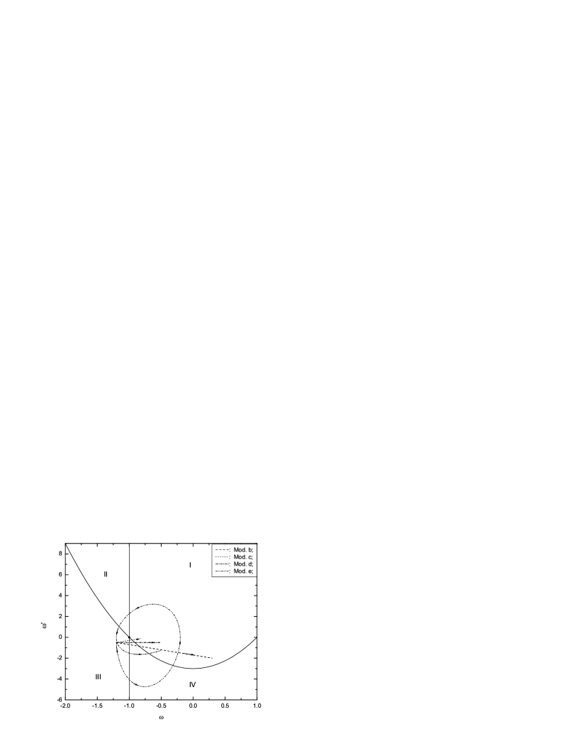
So the $\omega$-$\omega^{\prime}$ plane is divided into four parts

I:       $c_{a}^{2}<1$   &   $\omega>-1$,     $\omega^{\prime}>-3(1-\omega)(1+\omega)$ ;

II:       $c_{a}^{2}>1$   &   $\omega<-1$,     $\omega^{\prime}>-3(1-\omega)(1+\omega)$ ;

III:       $c_{a}^{2}<1$   &   $\omega<-1$,     $\omega^{\prime}<-3(1-\omega)(1+\omega)$ ;

IV:       $c_{a}^{2}>1$   &   $\omega>-1$,     $\omega^{\prime}<-3(1-\omega)(1+\omega)$ .
This can be seen clearly in Fig. [1]. From Eq. (38), one can easily find that $\dot{V}<0$ is satisfied in Region I and II, the field rolling down the potential, and $\dot{V}>0$ is satisfied in Region III and IV, the field climbing up the potential. So from the value of the function $\omega^{\prime}+3(1-\omega)(1+\omega)$ being positive or negative, one can immediately judge how the field evolves at that time. This is one of the most important results in this section. In the case of $Q=0$, the hessence returns to the quintessence field, and conditions of $c_{a}^{2}<1$ and $\omega>-1$ are always satisfied. So only Region I is allowed, and the bound of $\omega^{\prime}>-3(1-\omega)(1+\omega)$ is satisfied, which is exactly same with Eq. (37). In the general case of $Q\neq 0$, these four regions are all allowed.

Now, let’s focus on the issue: how the EoS crosses $-1$ in the $\omega$-$\omega^{\prime}$ plane? Assuming at some time, the hessence being in Region I with $\omega>-1$ and $c_{a}^{2}<1$, there are two ways for the field to run to the regions with $\omega<-1$:

a) One is that, the field runs across the Critical Point $(\omega,\omega^{\prime})=(-1,0)$, and arrives in Region II or III. Unfortunately, this can’t be realized in finite time. We use Taylor expansion of $\omega^{\prime}$ at the state around the Critical Point, and keep the first two terms,

$$\omega^{\prime}=\left.\omega^{\prime}\right|_{-1}+\left.\frac{\partial\omega^{\prime}}{\partial\omega}\right|_{-1}(\omega+1)\equiv b(\omega+1)~{},$$

where $b$ is a constant number. Using the definition of $\omega^{\prime}$, this equation yields that $|\omega+1|=a^{b}$. It is possible to get $\omega=-1$ at $a\neq 0$, only if $b<0$ is satisfied. In this condition, only if $a\rightarrow\infty$, $\omega=-1$ can be got. So the hessence field can’t cross the Critical Point in finite time.

b) The other way is to cross the dot line and arrive in Region II. This is the only way for the hessence field to cross the state of $\omega=-1$. From Eq. (38), one can easily get

$$c_{a}^{2}=\omega-\frac{\omega^{\prime}}{3(1+\omega)}~{}.$$ (43)

When $\omega=-1$ and $\omega^{\prime}\neq 0$,  $c_{a}^{2}$ is divergent. In section $6$, we will prove that this divergence doesn’t yield the physical divergence of the perturbations of the dark energy.

At last, we discuss the possible late time attractor solutions of the hessence field. There are three kinds of solutions:  a)  The hessence has not an oscillating EoS and the late time attractor is phantom-like with $\omega<-1$. Since $\omega^{\prime}=0$ is satisfied for the attractor, this solution must be in the Region III;  b)  For the similar reason, if the attractor is quintessence-like with $\omega>-1$, it must stay in Region I;  c)  The other possibility is the $\Lambda$-like attractor. In this case, the hessence will run to the Critical Point $(\omega,\omega^{\prime})=(-1,0)$. But the phantom-like attractor is difficult to realize. From the expressions of the pressure $p$ and the energy density $\rho$ of the hessence, one knows that only if $\frac{1}{2}\dot{\phi}^{2}<\frac{Q^{2}}{2a^{6}\phi^{2}}$, the attractor is phantom-like. If $\dot{|\phi|}>0$ is satisfied for the attractor, the value of $\frac{Q^{2}}{2a^{6}\phi^{2}}$ will damp quickly with time, and at last, it is always unavoidable to arrive at $\frac{1}{2}\dot{\phi}^{2}>\frac{Q^{2}}{2a^{6}\phi^{2}}$, which is the quintessence-like result; on the other hand, if $\dot{|\phi|}<0$ is satisfied for the attractor, it is inevitable to run to the state of $|\phi|=0$, which is forbidden by the definition of the hessence model. So in the hessence models, the Big Rip is avoided naturally, which has been discussed in some special examples in Ref. [17].

Now, let’s discuss the hantom model in the similar way. The pressure and energy density of the hantom are

$$p=-\frac{1}{2}\dot{\phi}^{2}+\frac{Q^{2}}{2a^{6}\phi^{2}}-V~{},~{}~{}~{}\rho=-\frac{1}{2}\dot{\phi}^{2}+\frac{Q^{2}}{2a^{6}\phi^{2}}+V~{},$$ (44)

respectively. And the state equation is

$$\omega=\left.\left[\frac{1}{2}\dot{\phi}^{2}-\frac{Q^{2}}{2a^{6}\phi^{2}}+V\right]\right/\left[\frac{1}{2}\dot{\phi}^{2}-\frac{Q^{2}}{2a^{6}\phi^{2}}-V\right]~{}.$$ (45)

The kinetic equation is

$$\ddot{\phi}+3H\dot{\phi}+\frac{Q^{2}}{a^{6}\phi^{3}}-\frac{dV}{d\phi}=0~{},$$ (46)

which follows that

$$\frac{\omega^{\prime}}{(1+\omega)(1-\omega)(1-c_{a}^{2})}>\frac{-3}{1-c_{a}^{2}}~{},$$ (47)

where $c_{a}^{2}$ is also defined by $c_{a}^{2}\equiv\dot{p}/\dot{\rho}$, and the relation (38) is also satisfied. So in the hantom models, we also can divide the $\omega$-$\omega^{\prime}$ plane into the exactly same four parts as in Fig. [1]. One can easily find that $\dot{V}<0$ is satisfied in Region I and II, the field rolling down the potential, and $\dot{V}>0$ is satisfied in Region III and IV, the field climbing up the potential. In the case of $Q=0$, the hantom returns to the phantom field, and the conditions of $c_{a}^{2}<1$ and $\omega<-1$ are always satisfied. So only Region III is allowed, and the bound of $\omega^{\prime}<-3(1-\omega)(1+\omega)$ is satisfied. For the similar reason as before, the late time attractor of hantom can be phantom-like (Region III) or $\Lambda$-like (Critical Point). The former can lead to the Big Rip at the late Universe. In the following sections, we only discuss the hessence models to avoid the Big Rip.

In this section, we discuss two kinds of special potentials of the hessence fields. One is the model with an exponential potential

$$V(\phi)=V_{0}e^{-\lambda\kappa\phi}~{},$$ (48)

where $\lambda$ is a dimensionless constant. The other is the model with a power law potential

$$V(\phi)=V_{0}(\kappa\phi)^{n}~{},$$ (49)

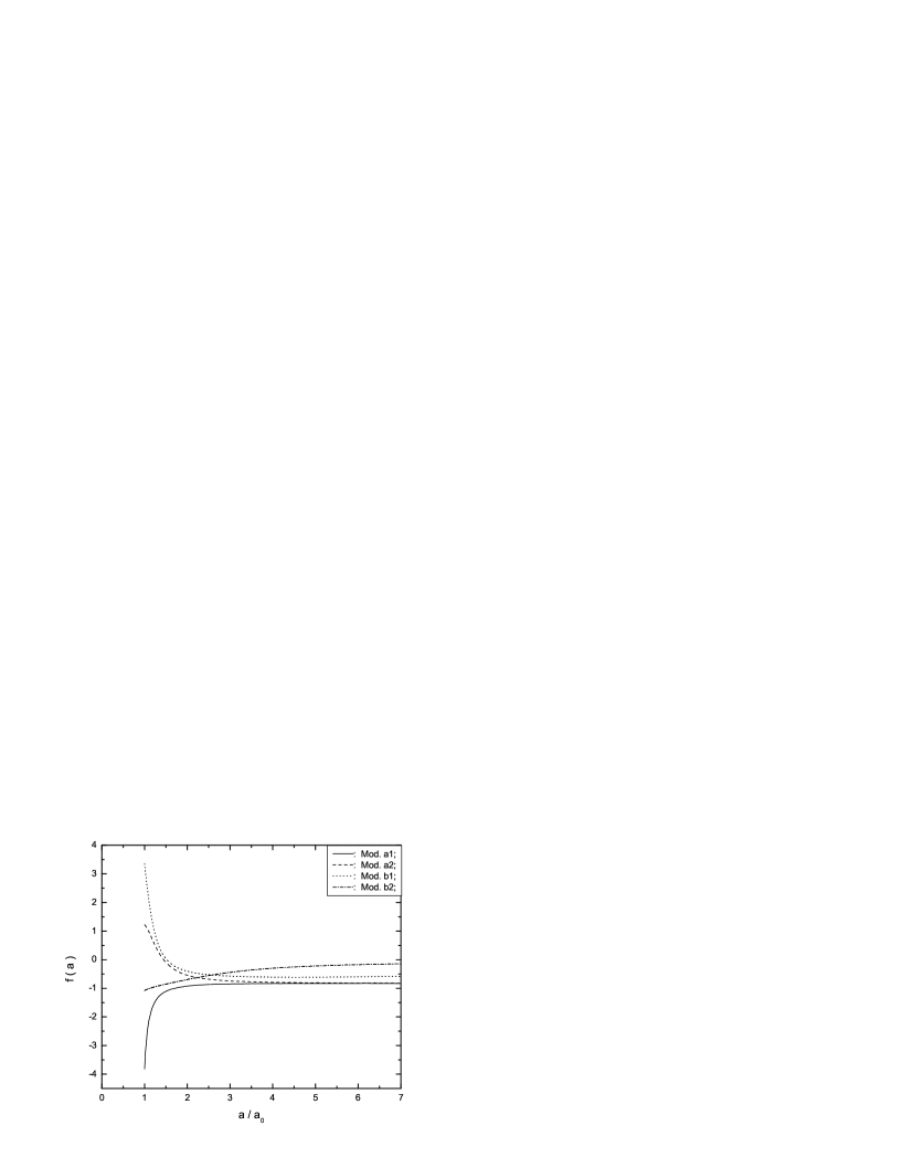
where $n$ is a dimensionless positive constant. These two forms of potentials are the most popular models, which are discussed in the scalar dark energy. In this section, we will numerically solve the kinetic equation of the hessence with these two kinds of potential functions, and study the evolution of $\omega$ and $\omega^{\prime}$ in detail to check the results we mentioned before. We focus on four special models:

Model a1: $\dot{\phi_{0}}>0$, $V(\phi)=V_{0}e^{-\lambda\kappa\phi}$ with $\lambda=1.0$, $Q^{2}/(\rho_{t}\phi_{0}^{2})=5$,  $\omega_{0}=-1.4$ ;

Model a2: $\dot{\phi_{0}}<0$, $V(\phi)=V_{0}e^{-\lambda\kappa\phi}$ with $\lambda=1.0$, $Q^{2}/(\rho_{t}\phi_{0}^{2})=0.5$,  $\omega_{0}=-0.7$ ;

Model b1: $\dot{\phi_{0}}>0$, $V(\phi)=V_{0}(\kappa\phi)^{n}$ with $n=2$, $Q^{2}/(\rho_{t}\phi_{0}^{2})=5$,  $\omega_{0}=-1.4$ ;

Model b2: $\dot{\phi_{0}}<0$, $V(\phi)=V_{0}(\kappa\phi)^{n}$ with $n=2$, $Q^{2}/(\rho_{t}\phi_{0}^{2})=0.5$,  $\omega_{0}=-0.7$ ,
where $\phi_{0}$ is the field $\phi$ with the present value, $\rho_{t}$ is the present total energy density, and $\omega_{0}$ is the present EoS of the hessence. In all these models, we choose the present density parameters $\Omega_{he0}=0.7$ and $\Omega_{m0}=0.3$. The first two models have the exponential potentials, and the latter two ones have power law potentials. The present EoS in Models a1 and b1 are phantom-like, and which are quintessence-like in Models a2 and b2. The EoS of the hessence is

$$\omega=\left.\left[\frac{1}{2}\dot{\phi}^{2}-\frac{Q^{2}}{2a^{6}\phi^{2}}-V(\phi)\right]\right/\left[\frac{1}{2}\dot{\phi}^{2}-\frac{Q^{2}}{2a^{6}\phi^{2}}+V(\phi)\right]~{}.$$ (50)

In Fig. [2], we plot their evolution in $\omega$-$\omega^{\prime}$ plane, and find that, except the Model b2, the behavior of $\omega$ crossing $-1$ exists in all these models. The Models a1 and a2 run to the same attractor solution of $(\omega,\omega^{\prime})=(-2/3,0)$, i.e. the quintessence-like solution, and the Models b1 and b2 run to the same point of $(\omega,\omega^{\prime})=(-1,0)$, i.e. the $\Lambda$-like solution. These results are same with the conclusion in Ref. [17], where the authors found that the hessence models with exponential potentials have the stable attractor solutions with $\omega=-1+\lambda^{2}/3$, and the models with power law potentials have the stable attractor solutions with $\omega=-1$. In these models, EoS crossing $-1$ obeys the second way: crossing the dot line (excluding the Critical Point $(\omega,\omega^{\prime})=(-1,0)$). So the divergence of the function $c_{a}^{2}$ exists.

In the $\omega$-$\omega^{\prime}$ plane, the Models a1 and b2 stay in the region I and II at all times, so the condition $\dot{V}<0$ holds for all time, and the fields roll down their potentials. But for the Models b1 and a2, they run from the regions with $\omega^{\prime}<-3(1+\omega)(1-\omega)$ to the ones with $\omega^{\prime}>-3(1+\omega)(1-\omega)$, so the fields climb up at the beginning and then roll down the potentials. These can be seen clearly in Fig. [3], where we plot the evolution of function $f\equiv\dot{V}/H\rho$ with the scale factor.

Generally, the observed EoS of dark energy is a function of redshift $z$, and the function form of $\omega(z)$ depends on the parametrized model. Now, how to know the potential function from the observed $\omega(z)$? If realized, it will be a direct way to relate the observation and dark energy models. In Ref. [21], the authors suggested a theoretical method of constructing the quintessence potential $V(\phi)$ directly from the state function $\omega(z)$. Since $\omega<-1$ can’t be realized in the quintessence models, this method is effective only for the state of $-1\leq\omega\leq 1$. But the recent observations mildly suggest that $\omega$ crossing $-1$ is existing. In this section, we will develop this method to construct the hessence potential $V(\phi)$ directly from $\omega(z)$. We apply this method to five typical parametrizations.

Consider the FRW Universe, which is dominated by the non-relativistic matter and a spatially homogeneous hessence field $\phi$. The Friedmann equation is

$$H^{2}=\frac{\kappa^{2}}{3}\left(\rho_{m}+\rho_{he}\right)~{},$$ (51)

where $\rho_{m}$ and $\rho_{he}$ are the densities of matter and hessence, respectively. The pressure, energy density and EoS of the hessence field have been written in Eqs. (24) and (25), from which we have

$$V(\phi)=\frac{1}{2}\left(1-\omega_{he}\right)\rho_{he}~{},$$ (52)

$$\dot{\phi}^{2}=\frac{Q^{2}}{a^{6}\phi^{2}}+(1+\omega_{he})\rho_{he}~{}.$$ (53)

These two equations relate the potential $V$ and field $\phi$ to the only function $\rho_{he}$. So the main task below is to solve the function form $\rho_{he}(z)$ from the parametrized EoS $\omega_{he}(z)$. The energy conservation equation of the hessence field is

$$\dot{\rho}_{he}+3H(\rho_{he}+p_{he})=0~{},$$ (54)

which yields

$$\rho_{he}(z)=\rho_{he0}\exp\left[3\int_{0}^{z}(1+\omega_{he})d\ln(1+z)\right]\equiv\rho_{he0}E(z)~{},$$ (55)

where the subscript $0$ denotes the value of a quantity at the redshift $z=0$ (present). In term of $\omega_{he}(z)$, the potential can be written as a function of the redshift $z$:

$$V[\phi(z)]=\frac{1}{2}(1-\omega_{he})\rho_{he0}E(z)~{}.$$ (56)

With the help of $\rho_{m}=\rho_{m0}(1+z)^{3}$ and Eq. (55), the Friedmann Eq. (51) becomes

$$H(z)=H_{0}\left[\Omega_{m0}(1+z)^{3}+\Omega_{he0}E(z)\right]^{1/2}~{},$$ (57)

where $\Omega_{m0}$ and $\Omega_{he0}$ are the present relativity densities of matter and hessence, respectively. Using Eq. (53), we have

$$\frac{d\phi}{dz}=\mp\frac{\left[\frac{Q^{2}}{a^{6}\phi^{2}}+(1+\omega_{he})\rho_{he}\right]^{1/2}}{(1+z)H(z)}~{},$$ (58)

where the upper (lower) sign applies if $\dot{\phi}>0~{}(\dot{\phi}<0)$. Here we choose the lower sign to avoid the state of $\phi=0$. It is helpful to define three dimensionless quantities $\tilde{\phi}$, $\tilde{V}$ and $C$

$$\tilde{\phi}\equiv\kappa\phi~{},~{}~{}~{}~{}~{}\tilde{V}\equiv V/\rho_{he0}~{},~{}~{}~{}~{}~{}C\equiv\kappa^{2}Q^{2}/\rho_{he0}~{}.$$ (59)

Eqs. (52) and (53) become

$$\frac{d\tilde{\phi}}{dz}=\frac{\sqrt{3}}{(1+z)}\left[\frac{C(1+z)^{6}\tilde{\phi}^{-2}+(1+\omega_{he})E(z)}{r_{0}(1+z)^{3}+E(z)}\right]^{1/2}~{},$$ (60)

$$\tilde{V}[\phi]=\frac{1}{2}(1-\omega_{he})E(z)~{},$$ (61)

where $r_{0}\equiv\Omega_{m0}/\Omega_{he0}$ is the energy density ratio of matter to hessence at present time. These two equations relate the hessence potential $V(\phi)$ to the EoS of the hessence $\omega_{he}(z)$. Given an effective $\omega_{he}(z)$, the construction Eqs. (60) and (61) allow us to construct the hessence potential $V(\phi)$. Here we consider the construction process with the following five parametrization methods.
The first model we consider is the EoS with constant value [22]:
Model a: $\omega_{he}=\omega_{0}$. If $\omega_{0}>-1$, a quintessence-like value, the construction of the potential can be easily realized with $Q\equiv 0$, where the hessence returns to the quintessence field. This condition has been discussed in Ref. [21]. Here we consider another case with $\omega_{0}=-1.2<-1$, a phantom-like value, and construct its potential function. In this case, the function $E(z)$ has a simple form

$$E(z)=(1+z)^{3(1+w_{0})}~{}.$$ (62)

Then we consider three two-parameter models [23, 24, 25]:
Model b: $\omega_{he}=\omega_{0}+\omega_{1}z$, and the function $E(z)$ has the form

$$E(z)=(1+z)^{3(1+w_{0}-w_{1})}e^{3w_{1}z}~{},$$ (63)

Model c: $\omega_{he}=\omega_{0}+\omega_{1}\frac{z}{1+z}$, and the function $E(z)$ has the form

$$E(z)=(1+z)^{3(1+w_{0}+w_{1})}e^{-3w_{1}\frac{z}{1+z}}~{},$$ (64)

Model d: $\omega_{he}=\omega_{0}+\omega_{1}\ln(1+z)$, and the function $E(z)$ has the form

$$E(z)=(1+z)^{3(1+w_{0})+\frac{3}{2}w_{1}\ln(1+z)}~{}.$$ (65)

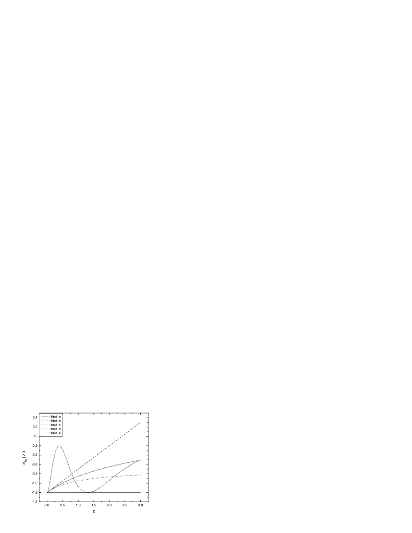
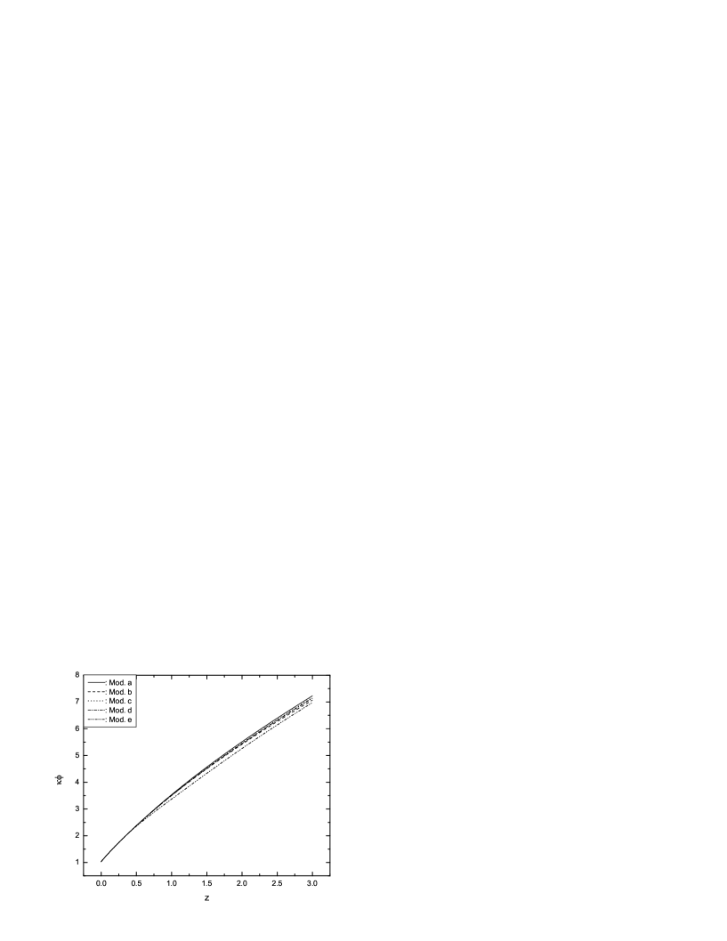
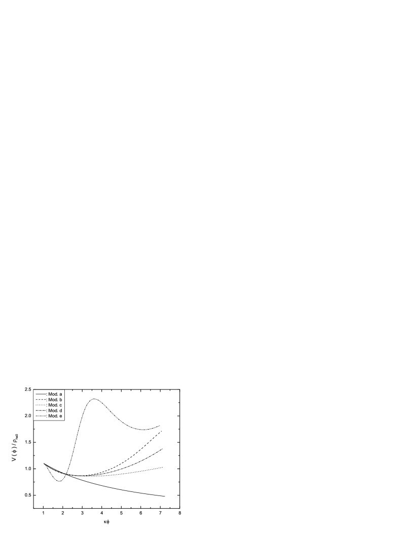
Inserting these into Eqs. (60) and (61), we can numerically evaluate the potential functions. In Fig. [4], we plot these parametrized EoS $\omega_{he}(z)$, where we have chosen the parameters $\omega_{0}=-1.2$, $\omega_{1}=0.5$. We find that, in the Models b, c and d, $\omega$ crossing $-1$ exists. In Fig. [5], we plot the evolution of $\phi$ with the redshift $z$, where we have chosen the parameters $r_{0}=3/7$, $C=5$ and the present value $\tilde{\phi}_{0}=1$. One finds, with the increasing of redshift, the values of $\phi$ monotonically increase in all these models. So the condition of $\phi=0$ is avoided.

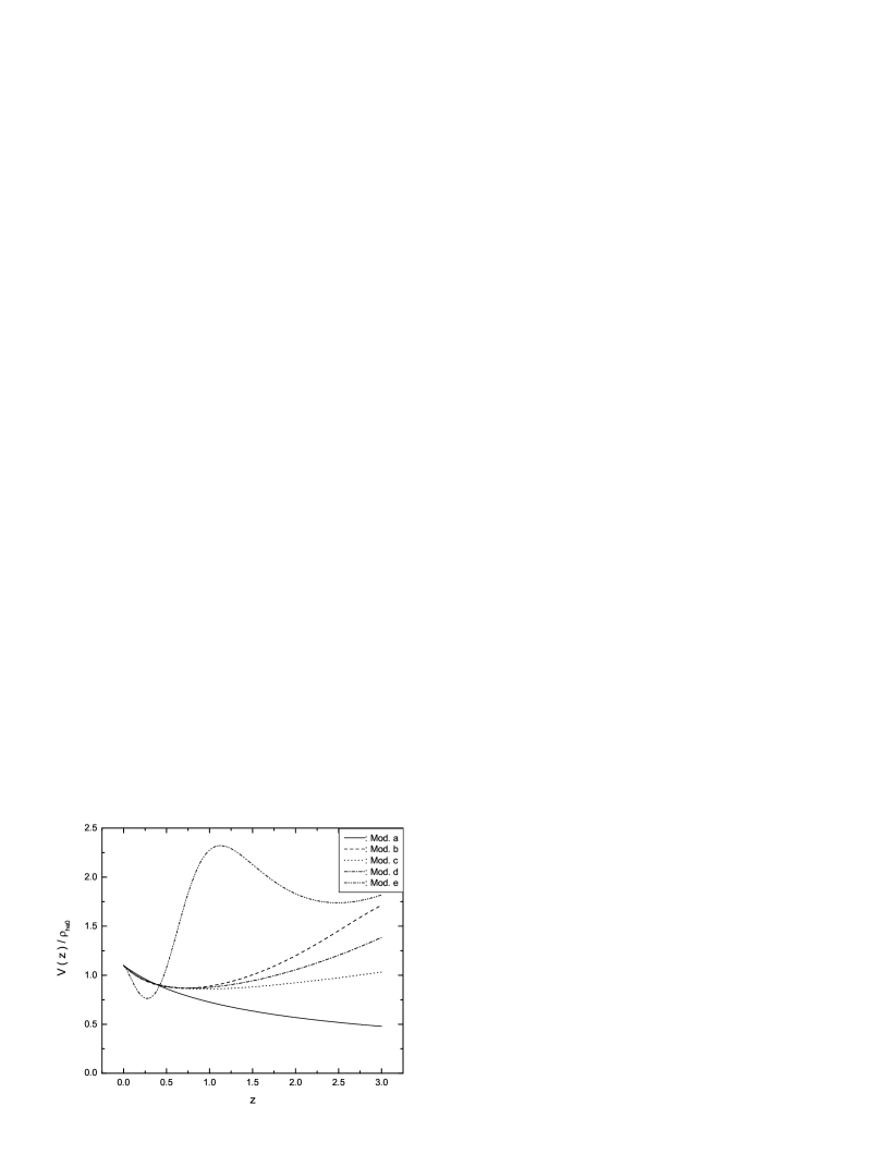
From Eq. (61), one can get the evolution of the potentials $V(z)$ of the hessence fields, which have been shown in Fig. [6]. From this figure, one finds the potential is climbed up for all time in the Model a. And in the Models b, c and d, the fields roll down the potentials at the higher redshift and climb up the potentials at the lower redshift. They all arrive at the lowest points of their potentials at the redshift, where $\omega_{he}^{\prime}+3(1-\omega_{he})(1+\omega_{he})=0$ is satisfied. These results are exactly what we expect: the Model a with $\omega_{he}<-1$ and $\omega^{\prime}_{he}=0$, stays in Region III in the $\omega_{he}$-$\omega_{he}^{\prime}$ plane, so $\dot{V}>0$ is satisfied for all time. But for the other models, we plot them in the $\omega_{he}$-$\omega_{he}^{\prime}$ plane in Fig. [7]. At the lower redshift, they all stay in Region III, which makes $\dot{V}>0$ is satisfied. And at the higher redshift, they all arrive in the Region I, where $\dot{V}<0$ is satisfied. Combining Eqs. (60) and (61), the potential functions $V(\phi)$ can be got, which have been shown in Fig.[8]. One finds these potentials are not monotonic functions of $\phi$, except the Model a, which are obviously different from the normal quintessence models [21].

Recently, a lot of authors have considered the dark energy with oscillating EoS [26]. They discussed that this kind of models give a naturally answer for the “coincidence problem” and “fine-tuning problem” of the dark energy. And in some models, it can naturally relate the early inflation and the recent accelerating expansion. The most interesting is that these models are likely to be marginally suggested by some observations [27]. The difficulty is that this kind of EoS is difficult to realize from the general potential function. Many periodic or nonmonotonic potentials have been put forward for quintessence fields, but rarely give rise to periodic $\omega(z)$. Here we consider a kind of oscillating parametrization:
Model e: $\omega_{he}=\omega_{0}+\omega_{1}\sin(\frac{1+z_{c}}{1+z})$. At the high redshift $z\gg z_{c}$, the oscillation of $\omega_{he}(z)$ disappears, and $\omega_{he}\simeq\omega_{0}$. The EoS is oscillating only when $z<z_{c}$. Here we choose parameters: $\omega_{0}=-0.7$ $\omega_{1}=0.5$ and $z_{c}=10$, so $\omega_{he}$ crossing $-1$ exists. And the present EoS is $\omega_{he0}=-1.2$, and $\omega_{he0}^{\prime}=0.5$, which are same to the values in Models b, c and d. The observations mildly suggest that the EoS of dark energy crossed $-1$ at very recent, which had been regarded as the second cosmological coincidence problem. The parametrization in Model e gives a naturally answer for this problem. Using this $\omega_{he}(z)$, we also can construct the potential of the hessence by applying the Eqs. (60) and (61), which has been plotted in Figs. [6] and [8]. We find although the potential $V(\phi)$ shows an oscillating behavior, this oscillation is different from the simple sine or cosine function, which appears at the pseudo-Nambu-Goldstone boson (PNGB) field [28] with the potential $V(\phi)=V_{0}[1+\cos(\phi/f)]$, where $f$ is a (axion) symmetry energy scale. Here the potential $V(\phi)$ of the hessence is an oscillating function with the increasing (or decreasing) amplitude. This suggests the method to build the potential of the scalar field dark energy, which can yield an oscillating EoS.

6. The Perturbations of the Quintom Fields

If the dark energy is a kind of dynamical field (or liquid), it is necessary to consider the perturbations of it. These studies have been done for many kinds of dark energy models, such as the quintessence fields, the phantom fields, the k-essence fields, and so on. Some models have predicted too large perturbations of the dark energy or the background metric. For example, the GCG models can produce the oscillations or exponential blowup of the matter power spectrum, which is inconsistent with observations [29]; the Yang-Mills field models have the imaginary sound speed, which makes the perturbations of the intrinsic spatial curvature $\Phi$ increasing rapidly at recent epoch [9]. For many models, which allows the existence of EoS crossing $-1$, the perturbations of the dark energy may be divergent at the state of $\omega_{de}=-1$ [30]. But whether or not, this divergence exists in our quintom models? In this section, we focus on this question by discussing the evolution of the perturbations of our quintom fields. In the conformal Newtonian gauge, the perturbed metric is given by

$$ds^{2}=a^{2}(\tau)\left[(1+2\Phi)d\tau^{2}-(1-2\Psi)dx^{i}dx_{i}\right]~{},$$ (66)

here we have used the conformal time $\tau$, which relates to the cosmic time by $dt\equiv ad\tau$. The gauge-invariant metric perturbation $\Psi$ is the Newtonian potential and $\Phi$ is the perturbation to the intrinsic spatial curvature. Always the background matters in the Universe are perfect fluids without anisotropic stress, which follows that $\Phi=\Psi$. So there is only one perturbation function $\Phi$ in the metric (66).

Using the notations of Ref. [31], the perturbations of the dark energy (including our quintom field) satisfy

$$\delta_{de}^{\prime}=-(1+\omega_{de})(\theta_{de}-3\Phi^{\prime})-3{\cal H}(c_{s}^{2}-\omega_{de})\delta_{de}~{},$$ (67)

$$\theta_{de}^{\prime}=-{\cal H}(1-3\omega_{de})\theta_{de}+3{\cal H}(c_{a}^{2}-\omega_{de})\theta_{de}+k^{2}\left(\frac{c_{s}^{2}}{1+\omega_{de}}\delta_{de}+\Phi\right)~{},$$ (68)

where ${\cal H}\equiv a^{\prime}/a$, and the ^′prime^′ denotes $d/d\tau$. $c_{s}$ is the sound speed of the dark energy, which is defined by $c_{s}^{2}\equiv\delta p_{de}/\delta\rho_{de}$, and its value can’t be larger than the light speed $c$. Here we have assumed zero anisotropic stress, which is the case for matter and simple dark energy models. The perturbation $\delta_{de}$ is defined by $\delta_{de}\equiv\delta\rho_{de}/\rho_{de}$, and $\theta_{de}$ is the divergence of the velocity of the dark energy. We should point out that both scalar fields and fluids obey the same forms of these two equations, and the only difference comes from the term of $c_{s}^{2}$. From Eq. (68), one can find that when $c_{a}^{2}\rightarrow\infty$, where $\omega_{de}=-1$ and $\omega_{de}^{\prime}\neq 0$ are satisfied, one will get infinite $\theta_{de}^{\prime}$. Fortunately, this divergence can’t lead to the divergence of $\delta_{de}$. It is helpful to define another function

$$\vartheta_{de}\equiv(1+\omega_{de})\theta_{de}~{},$$ (69)

then Eqs. (67) and (68) become

$$\delta_{de}^{\prime}=-\vartheta_{de}+3\Phi^{\prime}(1+\omega_{de})-3{\cal H}(c_{s}^{2}-\omega_{de})\delta_{de}~{},$$ (70)

$$\vartheta_{de}^{\prime}=-{\cal H}(1-3\omega_{de})\vartheta_{de}+k^{2}c_{s}^{2}\delta_{de}+k^{2}(1+\omega_{de})\Phi~{}.$$ (71)

We find that the divergence at $\omega_{de}=-1$ disappears. For the hessence field, we have

$$\delta\rho_{he}=\dot{\phi}\dot{(\delta\phi)}+\frac{Q^{2}\delta\phi}{a^{6}\phi^{3}}+\frac{dV}{d\phi}\delta\phi-\Phi\dot{\phi}^{2}~{},$$ (72)

$$\delta p_{he}=\dot{\phi}\dot{(\delta\phi)}+\frac{Q^{2}\delta\phi}{a^{6}\phi^{3}}-\frac{dV}{d\phi}\delta\phi-\Phi\dot{\phi}^{2}~{}.$$ (73)

In the frame where the perturbations of the scalar field $\delta\phi$ and $\dot{(\delta\phi)}$ are negligible, the sound speed of the quintom becomes $c_{s}^{2}\simeq 1$. So Eqs. (70) and (71) become

$$\delta_{he}^{\prime}=-\vartheta_{he}+3\Phi^{\prime}(1+\omega_{he})-3{\cal H}(1-\omega_{he})\delta_{he}~{},$$ (74)

$$\vartheta_{he}^{\prime}=-{\cal H}(1-3\omega_{he})\vartheta_{he}+k^{2}\delta_{he}+k^{2}(1+\omega_{he})\Phi~{}.$$ (75)

In general the evolution of the perturbations can be numerically computed, which depends on the component in the Universe and the special quintom models. For a complete study on the perturbations, the evolution of the metric perturbation $\Phi$ should also been considered, which satisfies the equation [32, 30]

$$\Phi^{\prime\prime}+3{\cal H}\left(1+\frac{p_{t}^{\prime}}{\rho_{t}^{\prime}}\right)\Phi^{\prime}+\frac{p_{t}^{\prime}}{\rho_{t}^{\prime}}k^{2}\Phi+\left[\left(1+3\frac{p_{t}^{\prime}}{\rho_{t}^{\prime}}\right){\cal H}^{2}+2{\cal H}^{\prime}\right]\Phi=4\pi Ga^{2}\left(\delta p_{t}-\frac{p_{t}^{\prime}}{\rho_{t}^{\prime}}\delta\rho_{t}\right)~{}.$$ (76)

The pressure $p_{t}\equiv\sum_{i}p_{i}$, and energy density $\rho_{t}\equiv\sum_{i}\rho_{i}$, which should include the contributions of baryon, photon, neutrino, cold dark matter, and dark energy. Especially at late time of the Universe, the effect of dark energy is very important. Combining the Eqs. (74), (75) and (76), one can numerically solve the function $\Phi(\tau)$ for special quintom models. Although we won’t calculate them in this paper, it also can be found that the value of $\Phi$ is finite as if the total function $p_{t}^{\prime}/\rho_{t}^{\prime}$ is finite. So even if $c_{a}^{2}\equiv p_{de}^{\prime}/\rho_{de}^{\prime}$ is divergent, $\Phi$ is also finite if only $p_{t}^{\prime}/\rho_{t}^{\prime}$ isn’t divergent. We should notice that, the Eqs. (74), (75) and (76) are also satisfied for the hantom models, where we only need to replace $\delta_{he}$ with $\delta_{ha}$, $\vartheta_{he}$ with $\vartheta_{ha}$, and $\omega_{he}$ with $\omega_{ha}$. We remind that the perturbations $\Phi$ and $\Psi$ can directly influence the CMB anisotropy power spectrum by the integral-Sachs-Wolfe (ISW) effect [33],

$$C_{l}^{ISW}\propto\int\frac{dk}{k}\left[\int_{0}^{\chi_{LSS}}d\chi~{}(\Phi^{\prime}+\Psi^{\prime})j_{l}(k\chi)\right]^{2}~{},$$ (77)

where $\chi_{LSS}$ is the conformal distance to the last scattering surface and $j_{l}$ the $l^{\prime}$th spherical Bessel function. The ISW effect occurs because photons can gain energy as they travel through time-varying gravitational wells. One always solves the power spectrum $C_{l}$ in the numerical methods [34], which can directly compare with the observations [2]. This is one of the most important way to study the dark energy models.

7. Conclusion

Understanding the nature of dark energy is one of the most important issues in the modern cosmology. Until recently, the most effective way is to detect the EoS $\omega_{de}$ and its time derivative $\omega_{de}^{\prime}$ by the observations on SNIa, CMB ,LSS and so on. There are mild evidences to show that $\omega_{de}$ crossing $-1$ exists at the very low redshift, which makes the building of the dark energy models difficult. A simple quintessence, phantom or k-essence field is insufficient. Although the states of $\omega_{de}\geq-1$ and $\omega_{de}\leq-1$ can be realized in these models, they all can’t give a state of $\omega_{de}$ crossing $-1$. A lot of more complex models have been suggested to account for this problem. Among them, the simplest one is the quintom model, which is a hybrid of quintessence and phantom fields. This kind of models have been discussed by a lot of authors. In this paper, we focused on a kind of special quintom, which has the potential $V(\phi_{1}^{2}-\phi_{2}^{2})$, where $\phi_{1}$ and $\phi_{2}$ are the quintessence and phantom fields, respectively. We investigated the general characters of this kind of models.

The lagrangian densities of the quintom are invariant under the hypergeometric transformation between the fields $\phi_{1}$ and $\phi_{2}$, which makes one can separate the quintom into two kinds: the hessence and the hantom. The former has the state of $\phi_{1}^{2}>\phi_{2}^{2}$, and the latter has the state of $\phi_{1}^{2}<\phi_{2}^{2}$. We discussed their evolution in the $\omega_{Q}$-$\omega_{Q}^{\prime}$ plane, and found this plane can be divided into four parts according to the values of $\dot{V}$ and $\omega_{Q}+1$ being larger or smaller than zero. The fact $\dot{V}>0~{}(<0)$ denotes that the potential of the quintom is climbed up (rolled down), and the fact $\omega_{Q}>-1~{}(<-1)$ denotes the field is quintessence-like (phantom-like). From their kinetic equations, we found $\omega_{Q}^{\prime}>-3(1-\omega_{Q})(1+\omega_{Q})$ is satisfied for the case of $\dot{V}<0$, and $\omega_{Q}^{\prime}<-3(1-\omega_{Q})(1+\omega_{Q})$ is satisfied when $\dot{V}>0$, which directly relates the evolution of potential to the value of EoS $\omega_{Q}$. We also found that, if the late time attractor solution exists, which is always quintessence-like or $\Lambda$-like for the hessence field, so the Big Rip is naturally avoided. But for hantom, this solution can be phantom-like or $\Lambda$-like. These characters are clearly shown in two hessence models with the exponential potential and power law potential.

In this paper, We also developed a theoretical method of constructing the hessence potential directly from the observable EoS $\omega_{he}(z)$. We applied our method to five kinds of parametrizations of EoS parameter, where $\omega_{he}$ crossing $-1$ can exist, and found they all can be realized in hessence models. Especially, the fifth model with the oscillating $\omega_{he}(z)$, we found although the potential $V(\phi)$ shows an oscillating behavior, this oscillation is different from the simple sine or cosine function. Here the potential $V(\phi)$ of the hessence is an oscillating function with the increasing (or decreasing) amplitude. In last part, we discussed the evolution of the perturbations of the quintom model, and found the perturbations of the quintom $\delta_{Q}$ and the metric $\Phi$ are all finite even if at the state of $\omega_{Q}=-1$ and $\omega_{Q}^{\prime}\neq 0$. We should notice that, in our discussion, we haven’t considered the possible interaction between the quintom field and the background matter, which may show some new interesting characters [17].

ACKNOWLEDGMENT: Zhang Yang’s research work has been supported by the Chinese NSF (10173008), NKBRSF (G19990754), and by SRFDP. Zhao Wen’s work is partially supported by Graduate Student Research Funding from USTC.

Figure 1: The $\omega$-$\omega^{\prime}$ plane of the hessence model. This plane is divided into four parts according to the values of $c_{a}^{2}-1$ and $\omega+1$ being larger or smaller than zero.

Figure 2: The evolution of four hessence models in $\omega$-$\omega^{\prime}$ plane. The thin arrows denote the evolutive direction of $\omega$ and $\omega^{\prime}$ with time.

Figure 3: The evolution of the function $\dot{V}(\phi)$ in the four hessence models. Here the dimensionless function $f(a)$ is defined by $f\equiv\frac{\dot{V}}{H\rho}$.

Figure 4: The EoS of five kinds of parametrization models.

Figure 5: Evolution of $\phi$ with the redshift $z$ of the hessence fields.

Figure 6: Evolution of potentials of the hessence models.

Figure 7: The parametrization models in $\omega$-$\omega^{\prime}$ plane. The thin arrows denote the evolutive direction of $\omega$ and $\omega^{\prime}$ with the increasing redshift $z$.

Figure 8: Constructed hessence potentials $V(\phi)$.

.

References

- [1] A.G.Riess et al., Astron.J. 116 (1998) 1009; S.Perlmutter et al., Astrophys.J. 517 (1999) 565; J.L.Tonry et al., Astrophys.J. 594 (2003) 1; R.A.Knop et al., Astrophys.J. 598 (2003) 102;
- [2] C.L.Bennett et al., Astrophys.J.Suppl. 148 (2003) 1; D.N.Spergel et al., Astrophys.J.Suppl. 148 (2003) 175; H.V.Peiris et al., Astrophys.J.Suppl. 148 (2003) 213; D.N.Spergel et al., arXiv:astro-ph/0603449;
- [3] M.Tegmark et al., Astrophys.J. 606 (2004) 702, M.Tegmark et al., Phys.Rev.D 69 (2004) 103501; A.C.Pope et al., Astrophys.J. 607 (2004) 655; W.J.Percival et al., MNRAS 327 (2001) 1297;
- [4] C.Wetterich, Nucl.Phys.B 302 (1988) 668 ; B.Ratra and P.J.E.Peebles, Phys.Rev.D 37 (1988) 3406; C.Wetterich, Astron.Astrophys. 301 (1995) 321; R.R.Caldwell, R.Dave and P.J.Steinhardt, Phys.Rev.Lett. 80 (1998) 1582;
- [5] C.Armendariz-Picon, T.Damour and V.Mukhanov, Phys.Lett.B 458 (1999) 209 ; T.Chiba, T.Okabe and M.Yamaguchi, Phys.Rev.D 62 (2000) 023511 ; C.Armendariz-Picon, V.Mukhanov and P.J.Steinhardt, Phys.Rev.D 63 (2001) 103510 ; L.P.Chimento, Phys.Rev.D 69 (2004) 123517 ; P.F.Gonzalez-Diaz, Phys.Lett.B 586 (2004) 1;
- [6] R.R.Caldwell, Phys.Lett.B 545 (2002) 23; S.M.Carroll, M.Hoffman and M.Trodden, Phys.Rev.D 68 (2003) 023509 ; R.R.Caldwell, M.Kamionkowski and N.N.Weinberg, Phys.Rev.Lett. 91 (2003) 071301 ; M.P.Dabrowski, T.Stachowiak and M.Szydlowski, Phys.Rev.D 68 (2003) 103519 ; V.K.Onemli and R.P.Woodard, Phys.Rev.D 70 (2004) 107301;
- [7] A.Y.Kamenshchik, U.Moschella and V.Pasquier, Phys.Lett.B 511 (2001) 265; N.Bilic, G.B.Tupper and R.D.Viollier, Phys.Lett.B 535 (2002) 17; M.C.Bento, O.Bertolami and A.A.Sen, Phys.Rev.D 66 (2002) 043507;
- [8] C.Armendariz-Picon, JCAP 0407 (2004) 007; V.V.Kiselev, Class.Quant.Grav. 21 (2004) 3323; H.Wei and R.G.Cai, Phys.Rev.D 73 (2006) 083002;
- [9] Y.Zhang Phys.Lett.B 340 (1994) 18; Y.Zhang, Gen.Rel.Grav. 34 (2002) 2155; Y.Zhang, Gen.Rel.Grav. 35 (2003) 689; Y.Zhang, Chin.Phys.Lett. 20 (2003) 1899; W.Zhao and Y.Zhang, arXiv:astro-ph/0508010; W.Zhao and Y.Zhang, arXiv:astro-ph/0604457;
- [10] U.Seljak et al., Phys.Rev.D 71 (2005) 103515; U.Seljak, A.Slosar and P.McDonald, arXiv:astro-ph/0604335;
- [11] P.S.Corasaniti, M.Kunz, D.Parkinson, E.J.Copeland and B.A.Bassett, Phys.Rev.D 70 (2004) 083006; S.Hannestad and E.Mortsell, JCAP 0409 (2004) 001; A.Upadhye, M.Ishak and P.J.Steinhardt, Phys.Rev.D 72 (2005) 063501 ; R.Lazkoz, S.Nesseris and L.Perivolaropoulos, JCAP 0511 (2005) 010;
- [12] A.Vikman, Phys.Rev.D 71 (2005) 023515;
- [13] D.F.Torres, Phys.Rev.D 66 (2002) 043522; S.Nojiri, S.D.Odintsov and S.Tsujikawa, Phys.Rev.D 71 (2005) 063004; R.R.Caldwell and M.Doran, Phys.Rev.D 72 (2005) 043527; S.Capozziello, S.Nojiri and S.D.Odintsov, Phys.Lett.B 634 (2006) 93; M.Z.Li, B.Feng and X.M.Zhang, JCAP 0512 (2005) 002; W.Zhao and Y.Zhang, Class.Quant.Grav. 23 (2006) 3405; E.J.Copeland, M.Sami and S.Tsujikawa, arXiv:hep-th/0603057; P.S.Apostolopoulos and N.Tetradis, arXiv:hep-th/0604014;
- [14] W.Hu, Phys.Rev.D 71 (2005) 047301; B.Feng, X.L.Wang and X.M.Zhang, Phys.Lett.B 607 (2005) 35;
- [15] Z.K.Guo, Y.S.Piao, X.M.Zhang and Y.Z.Zhang, Phys.Lett.B 608 (2005) 177; X.F.Zhang, H.Li, Y.S.Piao and X.M.Zhang, Mod.Phys.Lett.A 21 (2006) 231;
- [16] I.Ya.Aref’eva, A.S.Koshelev and S.Yu.Vernov, Phys.Rev.D 72 (2005) 064017;
- [17] H.Wei, R.G.Cai and D.F.Zeng, Class.Quant.Grav. 22 (2005) 3189; H.Wei and R.G.Cai, Phys.Rev.D 72 (2005) 123507; M.Alimohammadi and H. Mohseni Sadjadi, Phys.Rev.D 73 (2006) 083527;
- [18] R.R.Caldwell and E.V.Linder, Phys.Rev.Lett. 95 (2005) 141301; R.J.Scherrer, Phys.Rev.D 73 (2006) 043502 ;
- [19] T.Chiba, Phys.Rev.D 73 (2006) 063501;
- [20] SNAP Collaboration, arXiv:astro-ph/0507458; SNAP Collaboration, arXiv:astro-ph/0507459;
- [21] Z.K.Guo, N.Ohta and Y.Z.Zhang, Phys.Rev.D 72 (2005) 023504;
- [22] S.Hannestad and E.Mortsell, Phys.Rev.D 66 (2002) 063508;
- [23] A.R.Cooray and D.Huterer, Astrophys.J. 513 (1999) L95;
- [24] M.Chevallier and D.Polarski, Int.J.Mod.Phys.D 10 (2001) 213; E.V.Linder, Phys.Rev.Lett. 90 (2003) 091301; T.Padmanabhan and T.R.Choudhury, MNRAS 344 (2003) 823;
- [25] B.F.Gerke and G.Efstathiou, MNRAS 335 (2002) 33;
- [26] S.Dodelson, M.Kaplinghat and E.Stewart, Phys.Rev.Lett. 85 (2000) 5276; B.Feng, M.Z.Li and X.M.Zhang, Phys.Lett.B 634 (2006) 101; J.Q.Xia, B.Feng and X.M.Zhang, Mod.Phys.Lett.A 20 (2005) 2409; G.Barenboim, O.Mena and C.Quigg, Phys.Rev.D 71 (2005) 063533; G.Barenboim and J.Lykken, Phys.Lett.B 633 (2006) 453; E.V.Linder, Astropart.Phys. 25 (2006) 167; S.Nojiri and S.D.Odintsov, arXiv:hep-th/0603062; W.Zhao, arXiv:astro-ph/0604459;
- [27] D.Huterer and A.Cooray, Phys.Rev.D 71 (2005) 023506; R.Lazkoz, S.Nesseris and L.Perivolaropoulos, JCAP 0511 (2005) 010; J.Q.Xia, G.B.Zhao, H.Li, B.Feng and X.M.Zhang, arXiv:astro-ph/0605366;
- [28] K.Freese, J.A.Frieman and A.V.Olinto, Phys.Rev.Lett. 65 (1990) 3233; F.C.Asams, J.R.Bond, K.Freese, J.A.Frieman and A.V.Olinto, Phys.Rev.D 47 (1993) 426; J.Frieman, C.Hill, A.Stebbins and I.Waga, Phys.Rev.Lett. 75 (1995) 2077;
- [29] H.Sandvik, M.Tegmark, M.Zaldarriaga and I.Waga, Phys.Rev.D 69 (2004) 123524;
- [30] G.B.Zhao, J.Q.Xia, M.Z.Li, B.Feng and X.M.Zhang, Phys.Rev.D 72 (2005) 123515;
- [31] C.P.Ma and E.Bertschinger, Astrophys.J. 455 (1995) 7;
- [32] P.J.E.Peebles and B.Ratra, Astrophys.J. 325 (1988) L17 ; J.Weller and A.M.Lewis, MNRAS 346 (2003) 987; C.Gordon and W.Hu, Phys.Rev.D 70 (2004) 083003;
- [33] R.K.Sachs and A.M.Wolfe, Astrophys.J. 1 (1967) 73;
- [34] U.Seljak and M.Zaldarriaga, Astrophys.J. 469 (1996) 437; A.Lewis, A.Challinor and A.Lasenby, Astrophys.J. 538 (2000) 473;