Quintessence models with an oscillating equation of state and their potentials

Abstract

In this paper, we investigate the quintessence models with an oscillating equation of state (EoS) and their potentials. From the constructed potentials, which have the EoS of $\omega_{\phi}=\omega_{0}+\omega_{1}\sin z$, we find they are all the oscillating functions of the field $\phi$, and the oscillating amplitudes are decreasing (or increasing) with $\phi$. From the evolutive equation of the field $\phi$, we find this is caused by the expansion of the universe. This also makes that it is very difficult to build a model whose EoS oscillates forever. However one can build a model with EoS oscillating for a period. Then we discuss three quintessence models, which are the combinations of the invert power law functions and the oscillating functions of the field $\phi$. We find they all follow the oscillating EoS.

I Introduction

Recent observations on the Type Ia Supernova (SNIa)sn , Cosmic Microwave Background Radiation (CMB)map and Large Scale Structure (LSS)sdss all suggest that the universe mainly consists of dark energy (73%), dark matter (23%) and baryon matter (4%). How to understand the physics of the dark energy is an important issue, which has the EoS of $\omega<-1/3$, and leads to the recent accelerating expansion of the universe. Several scenarios have been put forward as a possible explanation of it. A positive cosmological constant is the simplest candidate, however it needs the extreme fine tuning to account for the observations. As the alternative to the cosmological constant, a number of dynamic models have been proposedphantom ; kessence ; quintom ; yangmills . Among them, the quintessence is the most natural modelquint , in which the dark energy is described by a scalar field $\phi$ with lagrangian density ${\cal L}_{\phi}=\frac{1}{2}\dot{\phi}^{2}-V(\phi)$. These models can naturally give the EoS with $-1\leq\omega_{\phi}\leq 1$. Usually, people discuss these models with monotonic potential functions i.e. the models with the exponential potentials and invert power law potentials. These models have some interesting characters, such as some models have late time attractor solutions with $\omega_{\phi}<0$simply , and some have the track solutions, which can naturally answer the cosmic “coincidence problem”track_quint . Recently, a number of authors have considered the dark energy with oscillating EoS in the quintessence modelsscott , in the quintom modelsosci , in the ideal-liquid models and in the scalar-tensor dark energy modelss-t . They discussed that this kind of dark energy may give a naturally answer for the “coincidence problem” and “fine-tuning problem”. And in some models, it is a naturally way to relate the very early inflation and recent accelerating expansion. The most interesting is that these models are likely to be marginally suggested by some observationsobservation .

In this paper, we will mainly discuss the quintessence models with the oscillating EoS. First, we construct the potentials from the parametrization $\omega_{\phi}=\omega_{0}+\omega_{1}\sin z$. We find these potentials are all the oscillating functions, and the oscillating amplitudes are increasing (decreasing) with the field $\phi$. This character can be analyzed from the evolutive equation of $\phi$. This suggests the way to build the potential functions which can follow the oscillating EoS. Then we discuss three kinds of potentials, which are the combinations of the invert power law functions and the oscillating functions, and find that they indeed give the oscillating EoS.

The plan of this paper is as follows: in Section 2, using the parametrized EoS $\omega_{\phi}=\omega_{0}+\omega_{1}\sin z$, we build their potentials, and investigate their general characters by discussing the kinetic equation of the quintessence field; then we build three kinds of models, and discuss the evolutions of their potentials, EoS and energy densities in Section 3; at last we will give a conclusion in Section 4.

We use the units $\hbar=c=1$ and adopt the metric convention as $(+,-,-,-)$ throughout this paper.

II Construction of the potentials

First, we will study the general characters of the potentials, which can follow the oscillating EoS. We note that many periodic or nonmonotonic potentials have been put forward for dark energy, but rarely give rise to the periodic $\omega_{\phi}(z)$. As one well-studied example, the potential for a pseudo-Nambu Goldstone boson (PNGB) fieldpngb can be written as $V(\phi)=V_{0}[\cos(\phi/f)+1]$, clearly periodic, where $f$ is a (axion) symmetry energy scale. However, unless the field has already rolls through the minimum, the relation $\omega_{\phi}(z)$ is monotonic and indeed can well described by the usual $\omega_{\phi}(a)=\omega_{0}+\omega_{1}(1-a)$. Then what kind of potentials can naturally give the oscillating EoS? In the Ref.scott , the authors built an example quintessence model, which has the potential $V(\phi)=V_{0}\exp(-\lambda\phi\sqrt{8\pi G})[1+A\sin(\nu\phi\sqrt{8\pi G})]$, where $\lambda$, $A$ and $\nu$ are all the constant numbers. They found that this model can indeed give an oscillating EoS, if choosing appropriate parameters. In this part, we will study the general characters of these models by constructing potential functions from the parametrized oscillating EoS. This method has been advised by Guo et al. in Ref.construct . First, we will give a simple review of this method.

The lagrangian density of the quintessence is

$${\cal L}_{\phi}=\frac{1}{2}\dot{\phi}^{2}-V(\phi).$$ (1)

and the pressure, energy density and EoS are

$$p_{\phi}=\frac{1}{2}\dot{\phi}^{2}-V(\phi),~{}~{}~{}~{}~{}\rho_{\phi}=\frac{1}{2}\dot{\phi}^{2}+V(\phi),$$ (2)

$$\omega_{\phi}\equiv\frac{p_{\phi}}{\rho_{\phi}}=\frac{\dot{\phi}^{2}-2V(\phi)}{\dot{\phi}^{2}+2V(\phi)}$$ (3)

respectively. When the energy transformation is from kinetic energy to potential energy, the value of $\omega_{\phi}$ is damping, and on the contrary, when the energy transformation is from potential energy to kinetic energy, the value of $\omega_{\phi}$ is raising. So the evolution of $\omega_{\phi}$ reflects the energy transformation relation of the quintessence field. This suggests the fact that it is impossible to get an oscillating EoS from the monotonic potentials, where the quintessence fields trend to run to the minimum of their potentials.

Consider the Flat-Robertson-Walker (FRW) universe, which is dominated by the non-relativistic matter and a spatially homogeneous quintessence field $\phi$. From the expression of the pressure and energy density of the quintessence field, we have

$$V(\phi)=\frac{1}{2}(1-\omega_{\phi})\rho_{\phi},$$ (4)

$$\frac{1}{2}\dot{\phi}^{2}=\frac{1}{2}(1+\omega_{\phi})\rho_{\phi}.$$ (5)

These two equations relate the potential $V$ and field $\phi$ to the only function $\rho_{\phi}$. So the main task below is to build the function form $\rho_{\phi}(z)$ from the parametrized EoS. This can be realized by the energy conservation equation of the quintessence field

$$\dot{\rho_{\phi}}+3H(\rho_{\phi}+p_{\phi})=0,$$ (6)

where $H$ is the Hubble parameter, which yields

$$\rho_{\phi}(z)=\rho_{\phi 0}\exp\left[3\int_{0}^{z}(1+\omega_{\phi})d\ln(1+z)\right]\equiv\rho_{\phi 0}E(z),$$ (7)

where $z$ is the redshift which is given by $1+z=a_{0}/a$ and subscript $0$ denotes the value of a quantity at the redshift $z=0$ (present). In term of $\omega_{\phi}(z)$, the potential can be written as a function of the redshift $z$:

$$V[\phi(z)]=\frac{1}{2}(1-\omega_{\phi})\rho_{\phi 0}E(z).$$ (8)

With the help of the Friedmann equation

$$H^{2}=\frac{\kappa^{2}}{3}(\rho_{m}+\rho_{\phi}),$$ (9)

where $\kappa^{2}=8\pi G$ and $\rho_{m}$ is the matter density, one can get

$$\tilde{V}[\phi]=\frac{1}{2}(1-\omega_{\phi})E(z),$$ (10)

$$\frac{d\tilde{\phi}}{dz}=\mp\sqrt{3}\frac{1}{(1+z)}\left[\frac{(1+\omega)E(z)}{r_{0}(1+z)^{3}+E(z)}\right]^{1/2},$$ (11)

where we have defined the dimensionless quantities $\tilde{\phi}$ and $\tilde{V}$ as

$$\tilde{\phi}\equiv\kappa\phi,~{}~{}~{}~{}~{}\tilde{V}\equiv V/\rho_{\phi 0},$$ (12)

and $r_{0}\equiv\Omega_{m0}/\Omega_{\phi 0}$ is the energy density ratio of matter to quintessence at present time. The upper (lower) sign in Eq.(11) applies if $\dot{\phi}>0(\dot{\phi}<0)$. These two equations relate the quintessence potential $V(\phi)$ to the equation of state function $\omega_{\phi}(z)$. Given an effective equation of state function $\omega_{\phi}(z)$, the construction Eqs.(10) and (11) will allow us to construct the quintessence potential $V(\phi)$.

Here we consider a most general oscillating EoS as

$$\omega_{\phi}=\omega_{0}+\omega_{1}\sin z,$$ (13)

where $|\omega_{0}|+|\omega_{1}|\leq 1$ must be satisfied for quintessence field. We choose the cosmological parameters as $\Omega_{\phi 0}=0.7$, and $\Omega_{m0}=0.3$. For the initial condition, we choose two different sets of parameters: case 1 with $\omega_{0}=-0.7$, $\omega_{1}=0.2$ and $\tilde{\phi}_{0}=1.0$; case 2 with $\omega_{0}=-0.4$, $\omega_{1}=0.5$ and $\tilde{\phi}_{0}=1.0$. We plot them in Fig.[1].

But how to fix the $``\mp"$ sign in Eq.(11)? We choose the initial condition with $d\tilde{\phi}_{0}/dz<0$, assuming the variety of this sign from $``-"$ to $``+"$ exists, then on the transformation point, (for the continue evolution of the field $\phi$) we have $\dot{\phi}=d\tilde{\phi}/dz=0$, which follows that $\omega_{\phi}=-1$ at this condition. Since $\omega_{\phi}>-1$ is always satisfied in these two models we consider, there is no transformation of the sign in Eq.(11). So the negative sign is held for all time. In Fig.[2], we have plotted the evolution of the potentials of the quintessence models with redshift, and in Fig.[3], we have plotted the constructed potentials. From these figures, one finds that although the potential functions are oscillating, but their amplitudes are altering with field. The field always runs from the potential with higher amplitudes to which with lower ones.

Now let’s analyze the reason of the these strange potential forms. The evolutive equation of the quintessence field is

$$\ddot{\phi}+3H\dot{\phi}+V_{,\phi}=0,$$ (14)

where $V_{,\phi}$ denotes $dV/d\phi$. This equation can be rewritten as

$$\ddot{\phi}+V_{,\phi}=-3H\dot{\phi}.$$ (15)

If the right-hand is absent, this is an equation which describes the motion of field $\phi$ in the potential $V(\phi)$ in the flat space-time. The right-hand of this equation is the effect of the expansion of the universe. Due to show clearly its effect on the field, we consider the simplest condition with $V(\phi)$ being a constant, if the right-hand is absent, we get that $\ddot{\phi}=0$, and $\dot{\phi}$ keeps constant, which is the free motion of the field. But if adding the right-hand, we get its solution $|\dot{\phi}|\propto e^{\int{-3Hdt}}$, the velocity of the field rapidly decreases with time. So the effect of the cosmic expansion is a kind of resistance to the field, and this force is directly proportionate to the velocity of the field $\dot{\phi}$. For overcoming this resistance force and keep the kinetic energy not being zero, the field must roll from the region with higher amplitude to the one with lower amplitude. This is the reason why the potential has so strange a form as shown in Figs.[2] and [3]. Since the field is always running to the relatively smaller value of its potential, but the potential can not be smaller than zero, it is very difficult to build the potential with EoS which oscillates forever if without extreme fine-tuning.

III Three quintessence models

From the previous section, we find the general characters of the potentials which can follow the oscillating EoS. According to these characters, one can find that the potential advised in ref.scott indeed satisfies this condition. However in that reference, the authors found a weak fine-tuning exists in the model for the constraint from the BBN observation. And also this model can obviously alter the CMB anisotropy power spectrum, compared to the standard $\Lambda$CDM model. These are bacause the oscillation of EoS exists at the radiation-dominant stage in that model. Here we will build another three kinds of potential functions, which also can generate the oscillating EoS. First we will simplify the evolutive equations of the quintessence field. We introduce the following dimensionless variables,

$$x\equiv\frac{\kappa\dot{\phi}}{\sqrt{6}H},~{}~{}y\equiv\frac{\kappa\sqrt{V}}{\sqrt{3}H},~{}~{}z\equiv\frac{\kappa\sqrt{\rho_{m}}}{\sqrt{3}H},~{}~{}u\equiv\frac{\sqrt{6}}{\kappa\phi},$$ (16)

then the evolutive equations of the matter and quintessence can be rewritten assimply

$$x^{\prime} = 3x(x^{2}+z^{2}/2-1)-f(y,u);$$ (17)

$$y^{\prime} = 3y(x^{2}+z^{2}/2)+f(y,u)x/y;$$ (18)

$$z^{\prime} = 3z(x^{2}+z^{2}/2-1/2);$$ (19)

$$u^{\prime} = -xu^{2},$$ (20)

where a prime denotes derivative with respect to the so-called e-folding time $N\equiv\ln a$, and the function $f(y,u)=\frac{\kappa V_{,\phi}}{\sqrt{6}H^{2}}$, which have the different forms for different potential functions. In this section, we mainly discuss three simple models, which have the similar potentials as in Fig.[3]:

Model 1: $V(\phi)=V_{0}(\kappa\phi)^{-2}[\cos(\phi/\phi_{c})+2]$ with $\kappa\phi_{c}=0.1$ and

$$f(y,u)=-uy^{2}-5\sqrt{6}y^{2}\sin(10\sqrt{6}/u)/[\cos(10\sqrt{6}/u)+2];$$ (21)

Model 2: $V(\phi)=V_{0}(\kappa\phi)^{-1}[\cos(\phi/\phi_{c})+2]$ with $\kappa\phi_{c}=0.1$ and

$$f(y,u)=-uy^{2}/2-5\sqrt{6}y^{2}\sin(10\sqrt{6}/u)/[\cos(10\sqrt{6}/u)+2];$$ (22)

Model 3: $V(\phi)=V_{0}[(\kappa\phi)^{-1}+\cos(\phi/\phi_{c})+1]$ with $\kappa\phi_{c}=0.1$ and

$$f(y,u)=-3y^{2}[u^{2}/6+10\sin(10\sqrt{6}/u)]/[u+\sqrt{6}+\sqrt{6}\cos(10\sqrt{6}/u)].$$ (23)

These models have been shown in Fig.[4], which all are the combinations of the invert power law function and the PNGB field. And $V(\phi)>0$ is satisfied for all time. When $\phi/\phi_{c}\ll 1$, they are like the invert power law potential with $n=-1($ or $-2)$, and they begin to oscillate when $\phi>\phi_{c}$. The oscillating amplitudes decrease for all time for the first two potentials, and for the last potential, the oscillating amplitudes are nearly a constant at $\phi\gg\phi_{c}$. It is interesting that these potentials can be looked as the invert power law potential $3V_{0}(\kappa\phi)^{-1}$ $(3V_{0}(\kappa\phi)^{-2},~{}V_{0}[(\kappa\phi)^{-1}+2])$ with an oscillating amendatory term at $\phi>\phi_{c}$. Here we choose the initial condition (present values) $\kappa\phi_{0}=0.6$, $\omega_{\phi 0}=-0.9$, $\Omega_{\phi 0}=0.7$ and $\Omega_{m0}=0.3$. So at the early stage, the potential functions of the quintessence are monotonic function, the EoS are not oscillating at the early (radiation-dominant) stage, which naturally overcome the shortcoming of the model in Ref.scott .

In Figs.[5] and [6], we plot the evolution of EoS and field $\phi$ in the region $\ln a/a_{0}=[0,4]$. The solid lines are the model with the first potential, whose EoS has a relatively steady oscillating amplitude. This is for the amplitudes in its potential function is rapidly decreasing with $\phi$. When the field $\phi$ rolls down to its valley, it has enough kinetic energy to climb up to its following hill and then rolls down again. At every period of its potential, when the field is rolling down, the kinetic energy is increasing, and the potential energy is decreasing, which makes its EoS is raising; on the contrary, when the field is climbing up, the kinetic energy is decreasing, and the potential energy is increasing, which makes its EoS is damping. The minimum values of its EoS never get $-1$, which is for the kinetic energy of the field never get zero. This process keeps until $\ln a/a_{0}\simeq 1.7$ ($\kappa\phi\simeq 2.2$), when the field gets the state with $\dot{\phi}=0$ ($\omega_{\phi}=-1$), and has to return to roll down the former valley ($\dot{\phi}<0$). These can be seen clearly in Fig.[6]. After this state, the EoS will rapidly run to a steady state with $\omega_{\phi}=-1$.

However all these are different for models 2 and 3, which are described with dash and dot lines in these figures. When the fields roll down to the valley with $\kappa\phi\simeq 1$, they try to climb up their first hills, however can not climb up to the peaks for the large values of their potential functions. When the fields get the state with $\dot{\phi}=0$, (the corresponding EoS are $\omega_{\phi}=-1$) they have to return to roll down this valley again. This process lasts until the kinetic energy become negligible, the fields stay at the valley with $\omega_{\phi}=-1$. The evolution of these fields can be seen clearly in Fig.[6].

In Fig.[7], we plot the evolution of $\Omega_{\phi}$ in the universe, although the quintessence will be dominant at last in the universe, the values of $\Omega_{\phi}$ are oscillating at the evolution stage for all these three quintessence models, which are determined by the evolution of $\omega_{\phi}$. When $\omega_{\phi}>0$, the values of $\Omega_{\phi}$ will decrease, and when $\omega_{\phi}<0$, the values of $\Omega_{\phi}$ will increase.

IV Conclusion

Understanding the physics of the dark energy is one of the most mission for the modern cosmology. Until recently, the most effective way is to detect its EoS and the running behavior by the observations on SNIa, CMB ,LSS and so on. There are mild evidences to show that the EoS of the dark energy is the oscillating function, which makes the building of the dark energy models difficult. For the quintessence field dark energy models, it is obvious that this EoS can’t be realized from the monotonic potentials. However for the simple oscillating potential, it is also difficult to realize.

In this paper, we have discussed the general features of the potentials which can follow an oscillating EoS by constructing the potentials from oscillating EoS, and found that they are oscillating functions, however the oscillating amplitudes are increasing (decreasing) with the field $\phi$. And also the field must roll from the region with larger amplitude to which with smaller amplitude if the EoS is oscillating. This kind of potentials are not very difficult to satisfy. However since the field must roll down to the region with smaller amplitude if the EoS is oscillating, and also the constraint of $V(\phi)\geq 0$ must be satisfied for all time, which lead to the building of quintessence with oscillating (forever) EoS is very difficult. In this paper, we have studied three kinds of models: $V(\phi)=V_{0}(\kappa\phi)^{-2}[\cos(\phi/\phi_{c})+2]$,  $V(\phi)=V_{0}(\kappa\phi)^{-1}[\cos(\phi/\phi_{c})+2]$ and $V(\phi)=V_{0}[(\kappa\phi)^{-1}+\cos(\phi/\phi_{c})+1]$. They are all made of the invert power law functions and the oscillating functions, and can indeed follow the oscillating EoS, however this oscillating behavior can only keep a finite period in all these three models.

Figure 1: The parametrized EoS $\omega_{\phi}(z)=\omega_{0}+\omega_{1}\sin z$.

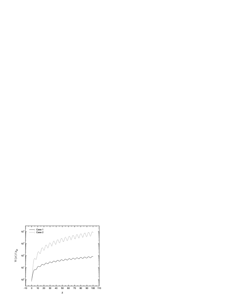
Figure 2: The evolution of the potentials of the quintessence models with redshift $z$.

Figure 3: Constructed potential functions

Figure 4: Three kinds of quintessence models.

Figure 5: The evolution of the EoS of the quintessence models.

Figure 6: The evolution of field $\phi$ of the quintessence models.

Figure 7: The evolution of the energy density $\Omega_{\phi}$ of the quintessence models.

References

- (1) Riess A.G. et al., Astron.J. 116 (1998) 1009; Perlmutter S. et al., Astrophys.J. 517 (1999) 565; Tonry J.L. et al., Astrophys.J. 594 (2003) 1; Knop R.A. et al., Astrophys.J. 598 (2003) 102;
- (2) Bennett C.L. et al., Astrophys.J.Suppl. 148 (2003) 1; Spergel D.N. et al., Astrophys.J.Suppl. 148 (2003) 175; Peiris H.V. et al., Astrophys.J.Suppl. 148 (2003) 213; Spergel D.N. et al., astro-ph/0603449;
- (3) Tegmark M. et al., Astrophys.J. 606 (2004) 702, Phys.Rev.D 69 (2004) 103501; Pope A.C. et al., Astrophys.J. 607 (2004) 655; Percival W.J. et al., MNRAS 327 (2001) 1297;
- (4) Caldwell R.R., Phys.Lett.B 545 (2002) 23; Carroll S.M., Hoffman M. and Trodden M., Phys.Rev.D 68 (2003) 023509; R.R.caldwell, M.Kamionkowski and N.N.Weinberg, Phys.Rev.Lett. 91 (2003) 071301;
- (5) Armendariz C., Damour T. and Mukhanov V., Phys.Lett.B 458 (1999) 209; Chiba T., Okabe T. and Yamaguchi M., Phys.Rev.D 62 (2000) 023511; Armendariz C., Mukhanov V. and Steinhardt P.J., Phys.Rev.D 63 (2001) 103510;
- (6) Feng B., Wang X.L. and Zhang X.M., Phys.Lett.B 607 (2005) 35; Guo Z.K., Piao Y.S., Zhang X.M. and Zhang Y.Z., Phys.Lett.B 608 (2005) 177; Hao W. and Cai R.G., Phys.Rev.D 72 (2005) 123507; Hu W., Phys.Rev.D 71 (2005) 047301;
- (7) Zhang Y., Chin.Phys.Lett. 20 (2003) 1899; Zhao W. and Zhang Y., Class.Quant.Grav. 23 (2006) 3405; Phys.Lett.B 640 (2006) 69; astro-ph/0508010; Zhang Y., Xia T.Y. and Zhao W., gr-qc/0609115;
- (8) Wetterich C., Nucl.Phys.B 302 (1988) 668 ; Astron.Astrophys. 301 (1995) 321; Ratra B. and Peebles P.J., Phys.Rev.D 37 (1988) 3406; Caldwell R.R., Dave R. and Steinhardt P.J., Phys.Rev.Lett. 80 (1998) 1582; Zhai X.H. and Zhao Y.B. Chin.Phys. 15 (2006) 1009;
- (9) Copeland E.J., Liddle A.R. and Wands D., Phys.Rev.D 57 (1998) 4686; Amendola L., Phys.Rev.D 60 (1999) 043501; Amendola L., Phys.Rev.D 62 (2000) 043511
- (10) Zlatev I., Wang L. and Steinhardt P.J. Phys.Rev.Lett. 82 (1999) 896; Steinhardt P.J., Wang L. and Zlatev I., Phys.Rev.D 59 (1999) 123504;
- (11) Dodelson S., Kaplinghat M. and Stewart E., Phys.Rev.Lett. 85 (2000) 5276;
- (12) Feng B., Li M.Z. and Zhang X.M., Phys.Lett.B 634 (2006) 101; Xia J.Q., Feng B. and Zhang X.M., Mod.Phys.Lett.A 20 (2005) 2409; Barenboim G., Mena O. and Quigg C., Phys.Rev.D 71 (2005) 063533; Barenboim G. and Lykken J., Phys.Lett.B 633 (2006) 453; Linder E.V., Astropart.Phys. 25 (2006) 167; Zhao W. and Zhang Y., Phys.Rev.D 73 (2006) 123509;
- (13) Nojiri S. and Odintsov S.D., Phys.Lett.B 637 (2006) 139;
- (14) Huterer D. and Cooray A., Phys.Rev.D 71 (2005) 023506; Lazkoz R., Nesseris S. and Perivolaropoulos L., JCAP 0511 (2005) 010; Xia J.Q., Zhao G.B., Li H., Feng B. and Zhang X.M., Phys.Rev.D 74 (2006) 083521;
- (15) Freese K., Frieman J.A. and Olinto A.V., Phys.Rev.Lett. 65 (1990) 3233; Asams F.C., Bond J.R., Freese K., Frieman J.A. and Olinto A.V., Phys.Rev.D 47 (1993) 426; Frieman J., Hill C., Stebbins A. and Waga I., Phys.Rev.Lett. 75 (1995) 2077; Copeland E.J., Sami M. and Tsujikawa S., hep-th/0603057;
- (16) Guo Z.K., Ohta N. and Zhang Y.Z., Phys.Rev.D 72 (2005) 023504; Li Hui, Guo Z.K. and Zhang Y.Z., Mod.Phys.Lett.A 21 (2006) 1683; Cao H.M., Xin X.B, Wang L. and Zhao W., Journal of Science and Technology of China accepted;