$\rm H\alpha$ OBSERVATIONS OF A LARGE SAMPLE OF GALAXIES AT $z\sim 2$:
IMPLICATIONS FOR STAR FORMATION IN HIGH REDSHIFT GALAXIES

Abstract

Using $\rm H\alpha$ spectra of 114 rest-frame UV-selected galaxies at $z\sim 2$, we compare inferred star formation rates (SFRs) with those determined from the UV continuum luminosity. After correcting for extinction using standard techniques based on the UV continuum slope, we find excellent agreement between the indicators, with $\langle\rm SFR_{\rm H\alpha}\rangle=31$ $\rm M_{\odot}\;{\rm yr}^{-1}$ and $\langle\rm SFR_{UV}\rangle=29$ $\rm M_{\odot}\;{\rm yr}^{-1}$. The agreement between the indicators suggests that the UV luminosity is attenuated by an typical factor of $\sim 4.5$ (with a range from no attenuation to a factor of $\sim 100$ for the most obscured object in the sample), in good agreement with estimates of obscuration from X-ray, radio and mid-IR data. The $\rm H\alpha$ luminosity is attenuated by a factor of $\sim 1.7$ on average, and the maximum $\rm H\alpha$ attenuation is a factor of $\sim 5$. In agreement with X-ray and mid-IR studies, we find that the SFR increases with increasing stellar mass and at brighter $K$ magnitudes, to $\langle\rm SFR_{\rm H\alpha}\rangle\sim 60$ $\rm M_{\odot}\;{\rm yr}^{-1}$ for galaxies with $K_{s}<20$; the correlation between $K$ magnitude and SFR is much stronger than the correlation between stellar mass and SFR. All galaxies in the sample have SFRs per unit area $\Sigma_{\rm SFR}$ in the range observed in local starbursts. We compare the instantaneous SFRs and the past average SFRs as inferred from the ages and stellar masses, finding that for most of the sample, the current SFR is an adequate representation of the past average. There is some evidence that the most massive galaxies ($M_{\star}>10^{11}$ $\rm M_{\odot}$) have had higher SFRs in the past.

1. Introduction

Recent studies have indicated that a large fraction of the stellar mass in the universe today formed at $z>1$ (Dickinson et al. 2003; Rudnick et al. 2003). Thus it is especially important to understand the rates and timescales of star formation in galaxies at high redshift. Effective techniques now exist for the selection of galaxies at $z\sim 2$; these use the galaxies’ observed optical (Steidel et al. 2004) or near-IR (DRGs, or Distant Red Galaxies with $J-K>2.3$; Franx et al. 2003) colors, or a combination of the two ($BzK$-selected galaxies, Daddi et al. 2004), and can be used to select both star-forming and passively evolving galaxies. Galaxies selected by their optical ($U_{n}G{\cal R}$) colors comprise $\sim 70$% of the star formation rate density at $z\sim 2$ (including $U_{n}G{\cal R}$ and $BzK$ galaxies to $K=22$ and DRGs to $K=21$), and range in bolometric luminosity from $\sim 10^{10}$ L_⊙ to $>10^{12}$ L_⊙ (Reddy et al. 2005, 2006). This paper focuses on the star formation properties of such galaxies.

Advances in instrumentation have enabled the determination of star formation rates at an increasing range of wavelengths. The most straightforward data to obtain are optical images, which sample the rest-frame UV at $z\sim 2$. The UV light is attenuated by dust, however, and the magnitude of this extinction must be understood in order to obtain accurate SFRs. At high redshift, extinction is most readily determined by the UV slope in combination with an extinction law such as that of Calzetti et al. (2000); such an approach has been found to represent adequately the average extinction of most $z\sim 2$ star-forming galaxies, although the UV slope may overpredict the extinction for the youngest objects and underpredict it for the reddest and dustiest galaxies (Reddy & Steidel 2004; Reddy et al. 2006; Papovich et al. 2005).

The UV light which is absorbed by dust is reradiated in the infrared, and thus the FIR luminosity provides a more direct estimate of the bolometric star formation rate for many galaxies. The FIR light can be directly detected at submillimeter wavelengths for only the most luminous $z\sim 2$ galaxies (e.g. Chapman et al. 2005), but it is possible to make use of correlations between the FIR and X-ray and radio emission to estimate SFRs for more typical galaxies (Reddy & Steidel 2004). Such average star-forming galaxies at $z\sim 2$ are not detected even in the deepest X-ray and radio images, however, so these techniques work primarily for stacked images which give only the average SFR of a sample. More recently, the Spitzer Space Telescope has enabled the detection of the rest-frame IR light from individual $z\sim 2$ galaxies, for the most direct determinations of bolometric SFRs (Papovich et al. 2005; Reddy et al. 2006). Such estimates are still somewhat indirect, requiring templates to convert from the observed 5–8.5 µm luminosity to the total infrared luminosity $L_{\rm IR}$; however, these conversions give good average agreement with X-ray and dust-corrected UV estimates of SFRs.

One of the most widely used star formation indicators in local galaxies is the $\rm H\alpha$ emission line, which traces the formation of massive stars through recombination in H II regions. This is one of the most instantaneous measures of the SFR, and it has the advantage of being particularly well-calibrated (e.g. Kennicutt 1998a; Brinchmann et al. 2004). However, it is much more difficult to apply at high redshift because the $\rm H\alpha$ line shifts into the near-IR for $z\gtrsim 0.5$. Previous studies of $\rm H\alpha$-determined SFRs at high redshift have therefore been limited to relatively small samples of a few to $\sim 20$ galaxies (Erb et al. 2003; van Dokkum et al. 2004; Swinbank et al. 2004). Regardless of sample size, these studies have demonstrated that the detection of $\rm H\alpha$ at $z\sim 2$ is quite feasible with an 8–10 m telescope for galaxies with SFRs greater than a few $\rm M_{\odot}\;{\rm yr}^{-1}$.

A galaxy’s star formation history is as important as its current star formation rate, but is considerably more difficult to determine. The time at which galaxies begin forming stars is fundamental to models of galaxy formation, and so we would like to know the ages of galaxies, both locally and at high redshift, and whether or not their current SFRs are representative of their past star formation rates. Constraints on the histories of galaxies can be obtained by modeling their integrated light as the sum of stellar populations of varying ages. This has been done for large samples of local galaxies (e.g. Brinchmann et al. 2004; Heavens et al. 2004), but at high redshifts it is found that population synthesis models with a variety of simple star formation histories provide adequate fits to the broadband SEDs (Papovich et al. 2001; Shapley et al. 2001, 2005). With a sufficiently large sample, however, statistically meaningful results may still be obtained. Here we take advantage of the largest sample of $\rm H\alpha$ spectra yet assembled at high redshift, in combination with stellar masses and ages from population synthesis modeling, to compare the current star formation rate with the estimated past average.

This paper is one of several presenting the analysis of the $\rm H\alpha$ spectra of 114 $z\sim 2$ galaxies selected by their rest-frame UV colors. The paper is organized as follows. In §2 we describe the selection of our sample, the observations, and our data reduction procedures. We briefly outline the modeling procedure by which we determine stellar masses and other stellar population parameters in §3. In §4 we calculate and compare star formation rates from $\rm H\alpha$ and rest-frame UV luminosities. §5 discusses constraints on timescales for star formation. We summarize our results in §6. Separately, Erb et al. (2006b) focus on the galaxies’ kinematics and on comparisons of stellar, dynamical and inferred gas masses, and Erb et al. (2006a) use the same sample of $\rm H\alpha$ spectra to construct composite spectra according to stellar mass to show that there is a strong correlation between increasing oxygen abundance as measured by the [N II]/$\rm H\alpha$ ratio and increasing stellar mass. Galactic outflows in this sample are discussed by Steidel et al. (2006, in preparation).

A cosmology with $H_{0}=70\;{\rm km}\;{\rm s}^{-1}\;{\rm Mpc}^{-1}$, $\Omega_{m}=0.3$, and $\Omega_{\Lambda}=0.7$ is assumed throughout. In such a cosmology, 1″ at $z=2.24$ (the mean redshift of the current sample) corresponds to 8.2 kpc, and at this redshift the universe is 2.9 Gyr old, or 21% of its present age.

2. Sample Selection, Observations and Data Reduction

The selection of the sample and our observing and data reduction procedures are described in detail by Erb et al. (2006b). We summarize the object selection briefly here. The galaxies discussed in this paper are drawn from the rest-frame UV-selected $z\sim 2$ spectroscopic sample described by Steidel et al. (2004). The candidate galaxies are selected by their $U_{n}G\cal R$ colors (from deep optical images discussed by Steidel et al. 2004), with redshifts then confirmed in the rest-frame UV using the LRIS-B spectrograph on the Keck I telescope. Galaxies were selected for $\rm H\alpha$ observations for a wide variety of reasons, and the $\rm H\alpha$ sample is not necessarily representative of the UV-selected sample as a whole; because we selected some galaxies based on their bright $K$ magnitudes or red ${\cal R}-K$ colors, and because our $\rm H\alpha$ detection rate is lower for galaxies that are very faint in $K$ (as discusssed in more detail by Erb et al. 2006b), the $\rm H\alpha$ sample is slightly more massive on average than the UV-selected $z\sim 2$ sample as a whole, though it spans the full range of properties covered by the total sample. The galaxies observed are listed in Table 1; their coordinates and photometric properties are given in Table 1 of Erb et al. (2006b).

For the purposes of comparisons with other surveys, 10 of the 87 galaxies for which we have $\rm H\alpha$ spectra and $JK_{s}$ photometry have $J-K_{s}>2.3$ (the selection criterion for the FIRES survey, Franx et al. 2003); this is similar to the $\sim$12% of UV-selected galaxies which meet this criterion (Reddy et al. 2005). 18 of the 93 galaxies for which we have $K$ magnitudes have $K_{s}<20$, the selection criterion for the K20 survey (Cimatti et al. 2002); this is a higher fraction than is found in the full UV-selected sample ($\sim 10$%), because we intentionally targeted many $K$-bright galaxies (Shapley et al. 2004). Five of the 10 galaxies with $J-K_{s}>2.3$ also have $K_{s}<20$.

2.1. Near-IR Spectra

The $\rm H\alpha$ spectra were obtained with the near-IR spectrograph NIRSPEC (McLean et al. 1998) on the Keck II telescope in low-resolution ($R\sim 1400$) mode, and reduced using the standard procedures described by Erb et al. (2003). We comment here on the flux calibration, which is the most difficult step in the process but is essential to the determination of star formation rates. Absolute flux calibration is subject to significant uncertainties, primarily due to slit losses from the seeing and imperfect centering of the object on the slit (objects are acquired via blind offsets from a nearby bright star). Because the exposures of the standard stars used as reference are not usually taken immediately before or after the science targets (primarily because the NIRSPEC detector suffers from charge persistence after observations of bright objects), the calibration may also be affected by differences in seeing and weather conditions between the science and calibration observations.

Several methods have been used to assess the accuracy of the flux calibration. Using a narrow-band image of the Q1700 field (centered on $\rm H\alpha$ at $z=2.3$, for observations of the proto-cluster described by Steidel et al. 2005), we have measured narrowband $\rm H\alpha$ fluxes for six of the objects in our sample, and find that the NIRSPEC $\rm H\alpha$ fluxes are $\sim 50$% lower. For those (relatively few) galaxies for which we detect significant continuum in the NIRSPEC spectra, we can compare the average flux density in the $K$ band with the broadband magnitudes. These tests indicate that the NIRSPEC fluxes are low by a factor of $\sim 2$ or more. We have also assessed the effects of losses from the slit and the aperture used to extract the spectra by constructing a composite two-dimensional spectrum of all the objects in the sample and comparing its spatial profile to the widths of the slit and our aperture. This test indicates losses of $\sim 40$%, although this figure represents a lower limit because our procedure of dithering the object along the slit and subtracting adjacent images results in the occasional loss of flux from extended wings.

Motivated by these tests, we have when noted applied a factor of two aperture correction for the determination of star formation rates and $\rm H\alpha$ equivalent widths. The correction is imprecise, as the fraction of flux lost undoubtedly varies from object to object, but application of the correction results in a closer approximation to the true average flux of the sample than leaving the fluxes uncorrected (as shown by the good agreement obtained between $\rm H\alpha$ SFRs and those determined at other wavelengths).

2.2. Near-IR and Mid-IR Imaging

We also make use of $J$-band and $K_{s}$-band images obtained with the Wide-field IR Camera (WIRC; Wilson et al. 2003) on the 5-m Palomar Hale telescope, and mid-IR images from the Infrared Array Camera (IRAC) on the Spitzer Space Telescope. These data and our reduction procedures are described by Erb et al. (2006b).

3. Model SEDs and Stellar Masses

We determine best-fit model SEDs and stellar population parameters for the 93 galaxies for which we have $K$-band magnitudes. Most of these (87) also have $J$-band magnitudes, and 35 (in the GOODS-N and Q1700 fields) have been observed at rest-frame near-IR wavelengths with IRAC. We use a modeling procedure identical to that described in detail by Shapley et al. (2005), with the exception that we employ a Chabrier (2003) initial mass function (IMF) rather than the Salpeter (1955) IMF used by Shapley et al. (2005). This results in stellar masses and star formation rates 1.8 times lower.

The method is reviewed by Erb et al. (2006b), and the results are presented in Table 2 of that paper. Using the solar metallicity Bruzual & Charlot (2003) population synthesis models and a variety of simple star formation histories of the form ${\rm SFR}\propto e^{(-t_{\rm sf}/\tau)}$, with $\tau=10$, 20, 50, 100, 200, 500, 1000, 2000 and 5000 Myr, as well as $\tau=\infty$ (i.e. constant star formation, CSF), we determine the values of the age, $E(B-V)$ (using the Calzetti et al. 2000 extinction law), star formation rate and stellar mass which best match the observed 0.3–8 µm photometry. The mean stellar mass is $3.6\times 10^{10}$ $\rm M_{\odot}$, and the median is $1.9\times 10^{10}$ $\rm M_{\odot}$. The mean age is 1046 Myr, and the median age is 570 Myr. The sample has a mean $E(B-V)$ of 0.16 and a median of 0.15. The mean SFR is 52 $\rm M_{\odot}$ yr^-1, while the median is 23 $\rm M_{\odot}\;{\rm yr}^{-1}$; the difference between the two reflects the fact that a few objects are best fit with high SFRs ($>300$ $\rm M_{\odot}\;{\rm yr}^{-1}$). We determine uncertainties through a series of Monte Carlo simulations which account for photometric uncertainties and degeneracies between age, reddening and star formation history. The simulations are described by Shapley et al. (2005). The resulting mean fractional uncertainties are $\langle\sigma_{x}/\langle x\rangle\rangle=0.7$, 0.5, 0.6 and 0.4 in $E(B-V)$, age, SFR and stellar mass respectively. We also briefly consider two-component models, to assess the possible presence of an older stellar population hidden by current star formation. As discussed in more detail by Erb et al. (2006b), we find that the data do not favor large amounts of hidden mass; the most plausible of the two-component models increase the total stellar masses by a factor of $\sim 2$–3, comparable to the uncertainties in the single component modeling.

4. Star Formation Rates

There are three methods of estimating star formation rates for most of the galaxies in the sample. In addition to the $\rm H\alpha$ luminosity, which will be used for the primary analysis in this paper, SFRs can be calculated from the rest-frame UV continuum and the normalization of the best-fit model SED (see §3; these last two methods both use the UV continuum, so are not independent). The correspondence of $\rm H\alpha$ luminosity with SFR in particular is especially useful because it is widely used in the local universe and has recently been studied in detail using large samples of galaxies from the SDSS (Hopkins et al. 2003; Brinchmann et al. 2004). $\rm H\alpha$ also provides a nearly instantaneous meaure of the SFR, because only stars with masses greater that 10 $\rm M_{\odot}$ and ages less than 20 Myr contribute significantly to the ionizing flux. We use the Kennicutt (1998a) transformation between $\rm H\alpha$ luminosity and SFR, which assumes case B recombination, a Salpeter IMF ranging from 0.1 to 100 $\rm M_{\odot}$ which we convert to a Chabrier IMF by dividing the SFRs by 1.8, and that all the ionizing photons are reprocessed into nebular line emission. Using maximum likelihood SFRs from the full set of nebular emission lines, Brinchmann et al. (2004) show that this approximation works well for an average star-forming galaxy, but that massive, metal rich galaxies produce less $\rm H\alpha$ luminosity for the same SFR than low mass, metal poor galaxies. This is probably a metallicity effect, as increased line blanketing in metal-rich stars decreases the number of ionizing photons. The galaxies studied here follow a trend similar to local galaxies in mass and metallicity, though probably offset to lower metallicities at a given stellar mass (Erb et al. 2006a). The largest dispersion in the conversion factor from $\rm H\alpha$ luminosity to star formation rate is found for the most massive and metal-rich local galaxies (see Figure 7, Brinchmann et al. 2004); if our sample does not contain galaxies with the highest metallicities observed in the local universe, then the dispersion in the conversion factor is probably less than our uncertainties from other sources, though we may be biased toward overestimating the SFR by $\sim 0.1$ dex.

In order to calculate SFRs from the UV continuum we use the observed $G$-band magnitude, which corresponds to a mean rest-frame wavelength of 1480 Å for the galaxies in our sample (except for the 5 galaxies at $z\sim 1.5$, for which the $U_{n}$ magnitude corresponds to $\sim 1500$ Å). We use the Kennicutt (1998a) conversion between 1500 Å luminosity and SFR, which assumes a timescale of $\sim 10^{8}$ years for the galaxy to reach its full UV continuum luminosity. Because $\rm H\alpha$ is sensitive to only the most massive stars, it is a more instantaneous measure of SFR than the UV continuum; however, for a constant SFR the continuum luminosity rises by a factor of only 1.6 between ages of 10 and 100 Myr, so even for the youngest objects the UV continuum will not severely underestimate the SFR. We again convert from a Salpeter to a Chabrier IMF.

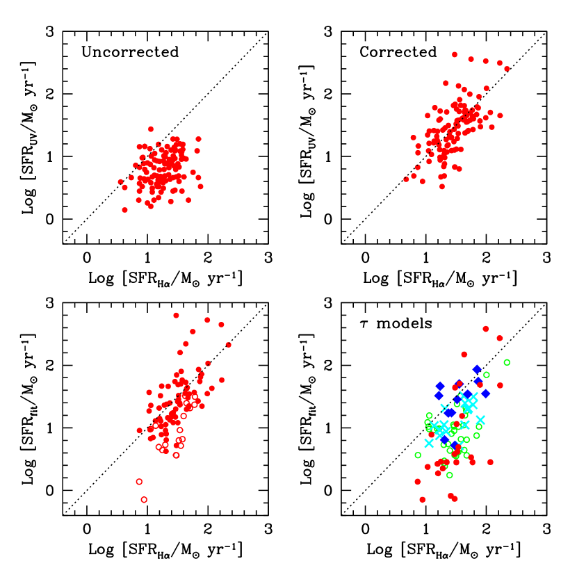
Figure 1.— A comparison of star formation rates from $\rm H\alpha$, the UV continuum, and the SED fits. Upper left: SFR_Hα vs. SFR_UV, without correcting for extinction. Upper right: SFR_Hα vs. SFR_UV, with both SFRs corrected for extinction. Lower left: Corrected SFR_Hα vs. the SFR obtained from the normalization of the adopted model SED. Solid symbols are constant star formation models, and the open symbols represent objects for which we have adopted a model with an exponentially decreasing star formation rate. Lower right: Corrected SFR_Hα vs. the SFR of the best-fitting declining model for each object. Filled red circles are galaxies with $\tau$=10, 20 or 50 Myr, open green circles have $\tau$=100, 200 or 500 Myr, cyan crosses have $\tau$=1, 2 or 5 Gyr, and blue diamonds are constant star formation models. The use of steeply declining $\tau$ models decreases the SFR with respect to that found from $\rm H\alpha$.

We compare the various SFRs in Figure 1. The upper left panel shows $\rm SFR_{UV}$ vs. $\rm SFR_{\rm H\alpha}$, without correcting for extinction (in all cases we apply a factor of two aperture correction to the $\rm H\alpha$ SFRs, as discussed in §2.1). There is considerable scatter, but the probability that the data are uncorrelated is $P=0.0006$, for a significance of the correlation of 3.4$\sigma$. We find a mean and standard deviation $\langle\rm SFR_{\rm H\alpha}\rangle=22\pm 14$ $\rm M_{\odot}\;{\rm yr}^{-1}$, and $\langle\rm SFR_{UV}\rangle=8\pm 5$ $\rm M_{\odot}\;{\rm yr}^{-1}$. In the upper right panel both fluxes have been corrected for extinction, using the Calzetti et al. (2000) extinction law and the best-fit values of $E(B-V)$ from the SED fits. For those galaxies which do not have SED fits because we lack the $K$ magnitude, $E(B-V)$ is calculated from the UV continuum slope as measured by the $G-{\cal R}$ color, assuming a 570 Myr old SED with constant star formation; this is the median best-fit age of the current sample. The value of $E(B-V)$ calculated from the $G-{\cal R}$ color in this way changes by less than 10% for assumed ages from 300–1000 Myr, though for young objects $E(B-V)$ will probably be underestimated using this method. The value of $E(B-V)$ used for each galaxy is shown in Table 1; the mean value is $\langle E(B-V)\rangle=0.16$. We have used the same value of $E(B-V)$ for the stellar UV continuum and for the nebular emission lines, rather than $E(B-V)_{\rm stellar}=0.4E(B-V)_{\rm neb}$ as proposed by Calzetti et al. (2000), because the latter assumption significantly overpredicts the $\rm H\alpha$ SFRs with respect to the UV SFRs. The relative extinction suffered by the stellar continuum and the nebular emission lines is an additional source of uncertainty in our SFRs. After the above corrections, we find a mean and standard deviation $\langle\rm SFR_{\rm H\alpha}\rangle=31\pm 18$ $\rm M_{\odot}\;{\rm yr}^{-1}$, and $\langle\rm SFR_{UV}\rangle=29\pm 19$ $\rm M_{\odot}\;{\rm yr}^{-1}$, using 3$\sigma$ rejection to compute the statistics in order to prevent the few objects with very high SFRs (particularly from the UV luminosity) from biasing the distribution.

The correlation between the corrected $\rm H\alpha$ and UV SFRs is highly significant (6.8$\sigma$), with an rms scatter of 0.3 dex. Some of this correlation may be due to the extinction correction applied to both SFRs; to test the significance of this effect, we have randomized the lists of uncorrected $\rm H\alpha$ and UV fluxes to create many sets of mismatched pairs, and applied the same (also randomized) value of $E(B-V)$ to both fluxes in each pair. In 10,000 trials we never observe a correlation as strong as that observed in the real data; the average trial has a correlation significance of 2.8$\sigma$ induced by the extinction correction. The much higher correlation significance in the real data confirms the underlying correlation of the uncorrected SFRs.

In the lower panels of Figure 1 we compare the corrected $\rm H\alpha$ SFRs with those determined by the normalization of the best-fitting SED. The SED modeling uses the extinction-corrected UV luminosity to determine SFRs, as we have done more directly in the comparison discussed above; the difference is that the modeling includes a variety of star formation histories. The primary purpose of this comparison is therefore to assess the effect of the assumed star formation history on SFRs determined from SED modeling. The lower left panel shows the SFR of our adopted best-fit model vs. $\rm SFR_{\rm H\alpha}$. The correlation is strong (5.3$\sigma$) and the rms scatter is 0.3 dex. The mean SFR from the SED fits is $\langle\rm SFR_{\rm fit}\rangle=24\pm 17$ $\rm M_{\odot}\;{\rm yr}^{-1}$, again computed with 3$\sigma$ rejection because of the few objects with very high SFRs. 70% of the objects have $\rm SFR_{\rm H\alpha}>SFR_{fit}$. The points with open circles are those for which we have used models with exponentially declining SFRs (SFR $\propto e^{-t/\tau}$) because they provided a significantly better fit than the constant star formation models; it is clear that the use of declining models depresses the SFR. This can be seen further in the lower right panel of Figure 1, in which we plot the SFR of the best-fitting declining model vs. $\rm SFR_{\rm H\alpha}$. The points are coded according to the value of $\tau$: filled red circles are those galaxies best fit with $\tau$=10, 20 or 50 Myr models, open green circles have $\tau$=100, 200 or 500 Myr, cyan crosses have $\tau$=1, 2 or 5 Gyr, and blue diamonds are constant star formation models. As expected, the steeply declining $\tau$ models yield the lowest SFRs, since they allow the SFR to drop significantly during the lifetime of massive stars. The objects with the highest SFRs are also formally best fit by steeply declining models; these are generally young, highly reddened objects that are acceptably fit by all values of $\tau$ and have high SFRs for all star formation histories. It is important to bear in mind when considering the $\tau$ models that they are undoubtedly an oversimplification of the likely star formation histories. A model with declining star formation may be required to obtain an acceptable fit when a galaxy shows significant light from a previous generation of stars as well as a current star formation episode, even if the current episode is best described by constant star formation. In such cases the current SFR is likely to be underestimated. Two component models which decouple the current star formation episode from the older population are more successful in determining current SFRs; general two-component models that add a linear combination of a current episode of constant star formation and an old burst (as described by Erb et al. 2006b) are significantly better at matching the $\rm H\alpha$-determined SFRs of galaxies which require $\tau$ models, while still providing an acceptable fit to the SED.

We conclude that a typical galaxy in our sample has a star formation rate of $\sim 30$ $\rm M_{\odot}\;{\rm yr}^{-1}$, though the SFRs of individual objects vary from $\sim 7$ to $\sim 200$ $\rm M_{\odot}\;{\rm yr}^{-1}$. The dispersion in the correlations suggest an uncertainty of a factor of $\sim 2$ for individual galaxies, as expected given the uncertainty of the aperture correction on individual objects. This result is in very good agreement with the mean SFR of $\sim 28$ $\rm M_{\odot}\;{\rm yr}^{-1}$ determined for the $z\sim 2$ UV-selected sample from X-ray stacking techniques (Reddy & Steidel 2004; Reddy et al. 2005; we have converted their value to a Chabrier IMF for comparison with our sample). We also find good agreeement between the $\rm H\alpha$ SFRs and those determined from 24 µm observations; Reddy et al. (2006) show that for $\sim 10$ galaxies in the GOODS-N field, the bolometric luminosities implied by the corrected $\rm H\alpha$ SFRs agree well with those inferred from the 24 µm luminosity.

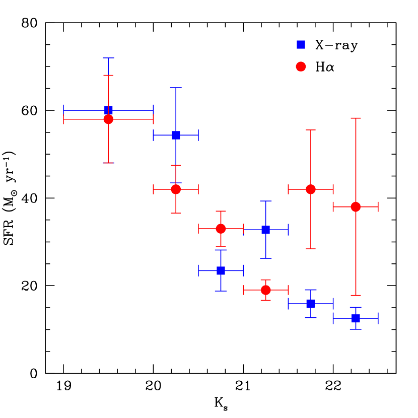
Figure 2.— Star formation rates from $\rm H\alpha$ and X-ray stacking, as a function of $K$ magnitude. Red circles from left to right represent the average extinction-corrected SFR_Hα of galaxies with $19<K_{s}\leq 20$ and in 0.5 magnitude bins between $K_{s}=20$ and $K_{s}=22.5$, excluding AGN. The average SFRs determined by stacking deep X-ray images of a slightly overlapping sample of $z\sim 2$ galaxies in the GOODS-N field in the same ranges of $K$ magnitude are shown by the blue squares (Reddy et al. 2005). The upturn in SFR_Hα at faint $K$ magnitudes is probably a selection effect, because we are less likely to detect $\rm H\alpha$ in galaxies faint in $K$ and because X-rays may underestimate the SFRs for young objects.

A further result of the Reddy et al. (2005) study is that the SFR increases with increasing $K$-band luminosity. We compare the current sample to the results of Reddy et al. (2005) by dividing our sample (excluding AGN) into bins in $K$ magnitude and finding the average corrected SFR_Hα in each bin. The results are shown in Figure 2, where the red circles are the average $\rm H\alpha$ SFRs and the blue squares are the SFRs from the X-ray stacking of Reddy et al. (2005). This is a comparison of similar objects, but not the same objects; the X-ray data are available only in the GOODS-N field, so the overlap between the two samples is small. The agreement is quite good for objects with $K\lesssim 21$, but the $\rm H\alpha$ data shows a rise in SFR for $K$-faint, low stellar mass objects that is not seen in the X-ray sample. This discrepancy is likely related to at least two different selection effects which complicate the comparison of SFRs at faint $K$ magnitudes. As noted in §2 and discussed in more detail by Erb et al. (2006b), we are less likely to detect $\rm H\alpha$ emission for objects that are faint in $K$, unless they have high SFRs. Factoring in non-detections of $K$-faint galaxies would probably lower the two right-most points considerably (we have not done this because of the difficulty in distinguishing non-detections due to low flux levels from non-detections for other reasons). If the low stellar mass objects in the $\rm H\alpha$ sample are young starbursts, the relative timescales of X-rays and $\rm H\alpha$ as star formation rate indicators may also be a factor. The $\rm H\alpha$ luminosity is nearly instantaneous, while the X-ray luminosity increases for the first $\sim 10^{8}$ years as O/B stars die and become high-mass X-ray binaries. The X-rays may thus underestimate the SFR for very young objects. Because the relative importance of these effects is difficult to quantify, the comparison of SFRs is most robust at brighter $K$ magnitudes, and the agreement between the $\rm H\alpha$, X-ray, UV and 24 µm SFRs in this range is encouraging. For the remaining analysis, we adopt the corrected $\rm H\alpha$ SFRs.

4.1. Star Formation Rate Surface Density

Because we have measured the spatial extent of the $\rm H\alpha$ emission (see Erb et al. 2006b) as well as the star formation rate it implies, we can also calculate the SFR surface density for the sample. After converting the SFRs to a Salpeter IMF by multiplying by 1.8 (for comparison with local galaxies), we find a mean $\langle\Sigma_{\rm SFR}\rangle=2.9$ $\rm M_{\odot}\;{\rm yr}^{-1}$ kpc^-2. As shown in Figure 3, the observed distribution is similar to the sample of local starburst galaxies studied by Kennicutt (1998b), with the exception that the $z\sim 2$ sample does not contain objects with $\Sigma_{\rm SFR}\gtrsim 20$ $\rm M_{\odot}\;{\rm yr}^{-1}$ kpc^-2; the upper cutoff of our distribution is an order of magnitude lower than is seen locally. The nearby galaxies with the highest values of $\Sigma_{\rm SFR}$ are the ultra-luminous IR galaxies (ULIRGs), which have bolometric luminosities $\gtrsim 10^{12}$ L_⊙. Recent 24 µm observations from the Spitzer Space telescope have shown that the most luminous $z\sim 2$ galaxies can be at least $\sim 10$ times more dust-obscured than would be inferred from their UV slopes (Reddy et al. 2006; Papovich et al. 2005). Thus it is possible that by using a UV-based extinction correction we have underestimated the SFRs for the most luminous galaxies in the sample, though by a smaller factor than we would using UV-based SFRs because of the lower optical depth for $\rm H\alpha$.

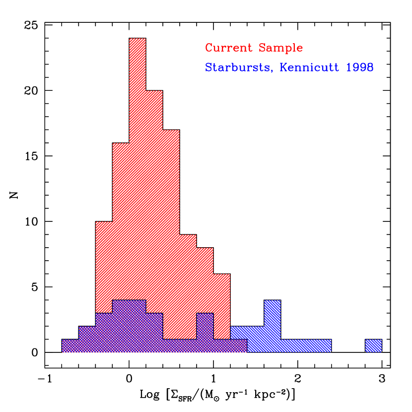
Figure 3.— A comparison of the star formation surface densities $\Sigma_{\rm SFR}$ of the current sample (large red histogram) and the starbursts of Kennicutt (1998b, shorter blue histogram). In this case we use a Salpeter IMF for consistency with the low redshift sample. The inability to resolve star formation on small spatial scales at high redshift results in an absence of objects with the highest values of $\Sigma_{\rm SFR}$ in the $z\sim 2$ sample.

However, the sample appears to include ULIRG-like objects. From the extinction-corrected $\rm H\alpha$ SFRs we estimate that the bolometric luminosities of the current sample range from $\sim 10^{11}$ to $\gtrsim 10^{12}$ L_⊙ (the bolometric luminosities inferred from $\rm H\alpha$ are plotted in Figure 10 of Erb et al. 2006b). Most of the local starbursts used by Kennicutt (1998b) are found in compact circumnuclear disks, with sizes smaller than the galaxy in which they are contained and smaller than the typical sizes we find for the $z\sim 2$ galaxies. It is not possible to resolve star formation on scales smaller than a few kpc in the high redshift sample; starburst activity that occurs in small, discrete regions rather than evenly across the galaxy would lead to an overestimate of the size and an underestimate of the surface density.

The large values of $\Sigma_{\rm SFR}$ imply high gas surface densities and substantial gas masses. This is discussed in detail by Erb et al. (2006b), in which we employ the correlation between $\Sigma_{\rm SFR}$ and gas density to estimate the galaxies’ gas masses and gas fractions, finding a mean gas fraction of $\sim 50$%. We also note that all of the objects have $\Sigma_{\rm SFR}>0.1$ $\rm M_{\odot}\;{\rm yr}^{-1}$ kpc^-2; starburst-driven superwinds are observed to be ubiquitous in galaxies with SFR densities above this threshold (Heckman 2002). The galaxies’ outflow properties are discussed by Steidel et al (2006, in preparation).

5. Comparisons with Stellar Mass and Star Formation Timescales

Given the suggestion of increasing SFR at brighter $K$ magnitudes shown in Figure 2 and found by Reddy et al. (2005), and the correlation between stellar mass and $K$, we might expect a correlation between SFR and stellar mass. This is tested in Figure 4, where in the left panel we show the extinction-corrected $\rm SFR_{\rm H\alpha}$ plotted against stellar mass. There is a general trend in the sense that objects with higher stellar masses have larger SFRs, but the data are only moderately correlated with a significance of 2.1$\sigma$. For the same set of objects, $K$ magnitude and SFR are much more strongly correlated, with 4.3$\sigma$ significance; this is probably because the rest-frame optical light is strongly affected by current star formation as well as the formed stellar mass.

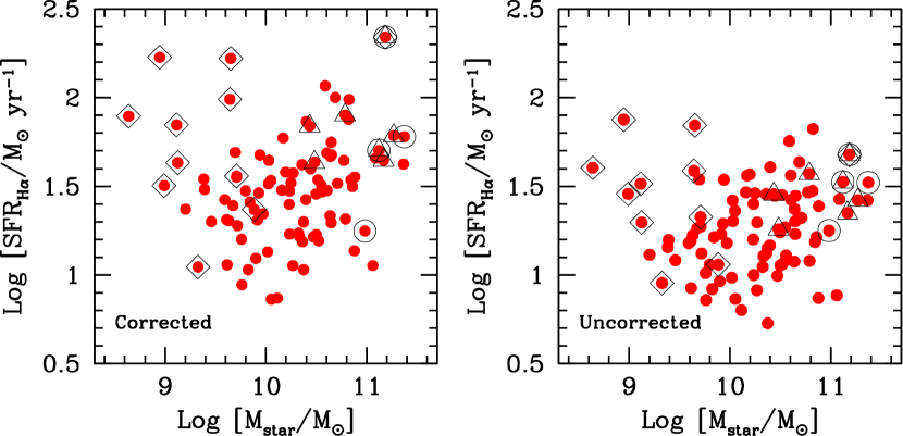
Figure 4.— Star formation rate from $\rm H\alpha$ vs. stellar mass, with the SFR corrected for extinction at left and uncorrected at right. In both cases SFR increases with increasing stellar mass, except for most of the galaxies with $M_{\rm dyn}/M_{\star}>10$ (marked with open diamonds; see Erb et al. 2006b). The absence of low mass galaxies with low SFRs is probably a selection effect, as such objects are less likely to be detected both in our $K$-band images and in $\rm H\alpha$. Massive galaxies with little current star formation would also not be present in our survey. Galaxies marked with triangles have $J-K>2.3$, and those marked with circles are AGN.

Some features of this plot can be explained by selection effects. The absence of objects with low stellar masses and low star formation rates is probably due to the fact that we are less likely to detect $\rm H\alpha$ in galaxies that are faint in $K$. A low mass galaxy would also require a relatively high SFR to be detected in the observed $K$-band. Massive, nearly passively evolving galaxies with low SFRs would also not be selected by our survey. This result can be usefully compared with that of Reddy et al. (2006), who consider bolometric luminosity as a function of stellar mass for optical and near-IR selected galaxies (Figure 14). They find that low mass galaxies span a wide range in bolometric SFRs, from LIRG to ULIRG levels of luminosity, and that the high mass and lower luminosity range of parameter space contains galaxies selected with near-IR techniques; thus, among galaxies of all types at $z\sim 2$, the correlation between stellar mass and SFR is relatively weak.

The points marked with open diamonds are objects in which the dynamical mass $M_{\rm dyn}$, as determined by the $\rm H\alpha$ line width and the spatial extent of the $\rm H\alpha$ emission, is more than 10 times larger than the stellar mass $M_{\star}$. Stellar and dynamical masses are compared by Erb et al. (2006b), who show that the galaxies with $M_{\rm dyn}/M_{\star}>10$ have young ages and high $\rm H\alpha$ equivalent widths, and are therefore likely to be young objects with large gas fractions. This conclusion is further strengthened by estimates of their gas masses, determined by making use of the correlation between star formation rate surface density and gas density (Kennicutt 1998b); the mean gas fraction implied for such $M_{\rm dyn}\gg M_{\star}$ objects is $\sim 90$%. These objects occupy a unique region in Figure 4, with high SFRs and low stellar masses.

A possible concern is that the high SFRs of the young, low mass objects are due to the extinction correction, if the degeneracy between age and extinction has caused an overestimation of the reddening. In the right panel of Figure 4 we plot the uncorrected $\rm SFR_{\rm H\alpha}$ vs. stellar mass, two entirely independently derived quantities; the plot is very similar to the corrected version, with the $M_{\rm dyn}/M_{\star}>10$ objects still among those with the highest SFRs in the sample. A related concern is that these young objects may not follow the same extinction law as the rest of the sample; this is suggested by Reddy et al. (2006), who show that (unlike most other UV-selected objects) galaxies with best fit ages $<100$ Myr are offset from the local relation between the UV slope $\beta$ and the ratio of far-IR to UV luminosity $L_{\rm FIR}/L_{1600}$. If this is true, the extinction correction may be overestimated for this set of objects. However, the impact on our results is negligible; we estimate that this could cause an overestimate of the SFRs in young objects of a factor of $\sim 1.2$, significantly less than other sources of uncertainty.

5.1. Star Formation Timescales

A commonly used measure of the importance of the current episode of star formation to the buildup of stellar mass in a galaxy is the specific star formation rate, the star formation rate per unit stellar mass. Massive galaxies have lower specific SFRs, and at a given stellar mass the specific SFR is observed to decline with redshift (e.g. Papovich et al. 2005; Reddy et al. 2006). We plot the specific SFR against stellar mass in Figure 5. This plot can be usefully compared with Figure 15 of Reddy et al. (2006), who plot specific SFR as a function of stellar mass for both UV and near-IR selected galaxies in the GOODS-N field. The higher fraction of massive galaxies in the NIRSPEC sample considered here shows that the UV-selected sample contains objects with stellar masses and specific SFRs comparable to the most massive near-IR selected objects with the lowest specific SFRs in the GOODS-N field (neglecting those which are not detected at 24 µm). Both figures show that at $z\sim 2$ (as in the local universe), galaxies with low stellar masses are assembling a much higher fraction of their stellar mass than more massive objects.

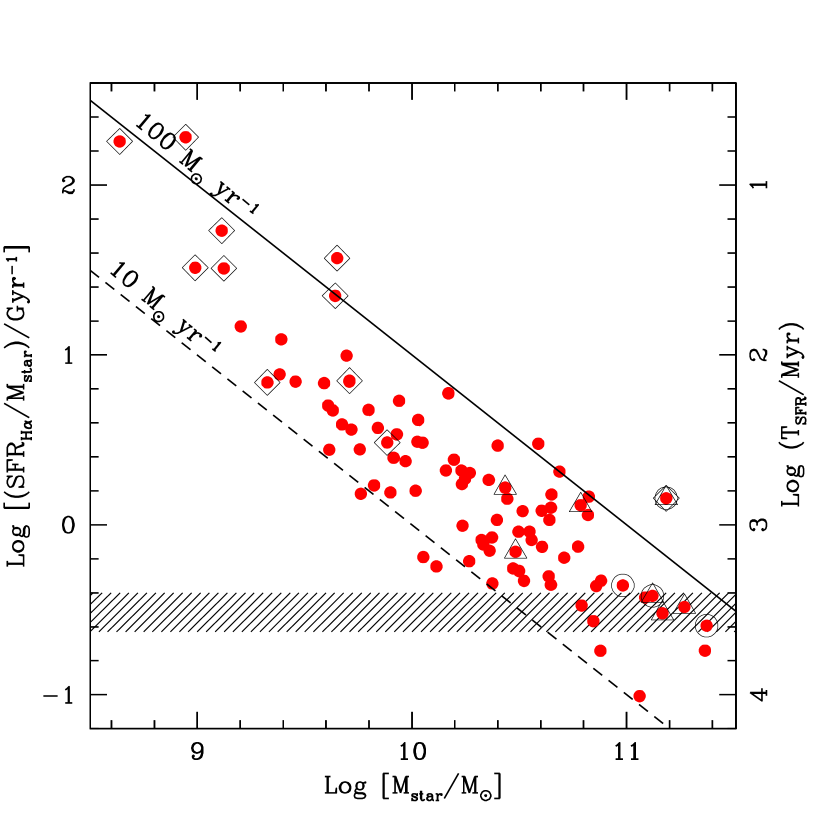
Figure 5.— The specific star formation rate SFR${}_{\rm H\alpha}/M_{\star}$ vs. stellar mass. The solid and dashed diagonal lines show star formation rates of 100 and 10 $\rm M_{\odot}\;{\rm yr}^{-1}$ respectively. The right axis shows the star formation rate timescale $T_{\rm SFR}=M_{\star}/{\rm SFR_{\rm H\alpha}}$, the inverse of the specific SFR. On this scale, the shaded band represents the age of the universe for the redshift range of the galaxies in the sample. The most massive galaxies have $T_{\rm SFR}\gtrsim t_{\rm universe}$, indicating that they may require declining star formation histories. Symbols are as in Figure 4.

The inverse of the specific SFR provides a star formation timescale, $T_{\rm SFR}=M_{\star}/\rm SFR$; this is the time required for the galaxy to form all its stellar mass at the current SFR. By comparison with the age of the universe at the redshift of the galaxy and with the inferred age from the SED fits, we may obtain some constraints on the star formation histories. The right axis of Figure 5 shows $T_{\rm SFR}$, and on this scale the shaded horizontal band represents the age of the universe for the range of redshifts in the sample. If $T_{\rm SFR}$ is greater than the age of the universe at the redshift of the galaxy, then the galaxy cannot have formed all its stars at the current rate, and must have had a higher SFR in the past. Only objects with $M_{\star}\gtrsim 6\times 10^{10}$ $\rm M_{\odot}$ have $T_{\rm SFR}$ approximately equal to the age of the universe. This upper limit on the time available for star formation suggests that while most objects do not require declining star formation histories, a CSF model may not be a reasonable fit for the most massive galaxies. These appear from Figure 5 to require higher past SFRs, although the uncertainties in the SFR and stellar masses are large enough that this conclusion is not robust. Similar results are found from the SED modeling, as noted in §3; the issue is discussed in more detail by Shapley et al. (2005), who find that constant star formation models do not provide an adequate fit to the SEDs of five of the six galaxies in their sample with $M_{\star}>10^{11}$ $\rm M_{\odot}$. These galaxies, and the most massive objects in the current sample, are best described by exponentially declining models with $\tau=1$–2 Gyr. With $\tau/t\gtrsim 1$, such a model would be indistinguishable from constant star formation for the younger galaxies in the sample, and may in fact be preferred for these objects because of the exponential SFR implied by a Schmidt law-like dependence of the star formation rate on the gas mass (see the discussion by Reddy et al. 2006).

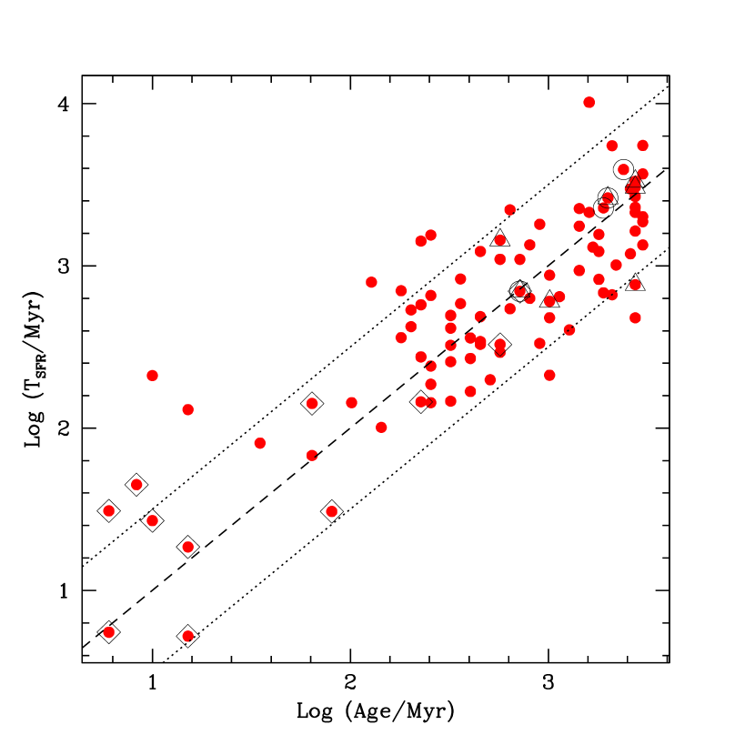
Figure 6.— The star formation timescale $T_{\rm SFR}$ vs. age. This plot provides a check of the consistency of the $\rm H\alpha$ SFRs and the primarily constant star formation models we use to fit the SEDs; for CSF models, $T_{\rm SFR}$ should be approximately equal to the age. The dashed line shows equal times, and the dotted lines on either side show the typical uncertainty in age. Symbols are as in Figure 4.

We can obtain additional constraints on the star formation histories by comparing $T_{\rm SFR}$ with the ages we obtain from the SED fitting. This test is implicit in the comparison of SFRs from $\rm H\alpha$ and the SED fitting shown in Figure 1; it is essentially a consistency check for our SED fits and $\rm H\alpha$ SFRs, since most of the ages represent constant star formation models. If the current SFR is an adequate representation of the past average, then $T_{\rm SFR}$ should be approximately equal to the age. We plot $T_{\rm SFR}$ vs. age in Figure 6. The dashed line represents equal timescales; if objects fall significantly above this line, they cannot have formed all of their stars at their current rate over their inferred lifetime and must have had a past burst, while objects significantly below the line would have a current SFR higher than the past average. The dotted lines show the average uncertainty in the age from our Monte Carlo simulations of the SED fits, which include uncertainties due to the star formation history. Most of the objects fall between or near the dotted lines, suggesting that constant star formation over the age determined by the SED fit adequately describes the star formation histories of most of the galaxies in our sample, though the scatter is certainly large enough to allow for some declining star formation histories, as may be required for the most massive galaxies. It should also be noted that the tendency of a few of the youngest galaxies to fall above the dashed line is probably due to an underestimate of their ages, which cannot realistically be less than their dynamical times; for this set of objects, the average $t_{\rm dyn}\simeq 2r/\sigma=80$ Myr (as compared to $\sim 130$ Myr for the entire sample).

5.2. $\rm H\alpha$ Equivalent Widths

The $\rm H\alpha$ equivalent width $W_{\rm H\alpha}$ provides an additional tool to investigate the star formation history. As the ratio of the $\rm H\alpha$ luminosity to the underlying stellar continuum, $W_{\rm H\alpha}$ is a measure of the ratio of the current to past average star formation. We determine $W_{\rm H\alpha}$ by taking the ratio of the $\rm H\alpha$ flux and the $K$-band continuum flux, after subtracting the contribution of $\rm H\alpha$ to the $K$-band magnitude. In calculating the equivalent widths we have applied the factor of two aperture correction to the $\rm H\alpha$ fluxes discussed above and in §2.1 (except in the cases of Q1623-BX455 and Q1623-BX502, for which twice the $\rm H\alpha$ flux slightly exceeds the $K$-band magnitude), but we have not applied an extinction correction; this is equivalent to the assumption that the nebular emission lines and the stellar continuum suffer the same attenuation. $W_{\rm H\alpha}$ is plotted against the best-fit age from the SED fits in Figure 7. For constant star formation, $W_{\rm H\alpha}$ should decrease with age, as the stellar continuum increases while the $\rm H\alpha$ flux remains the same. There is considerable scatter in the $W_{\rm H\alpha}$–age comparison, but the probability that the data are uncorrelated is $P=0.001$, for a significance of 3.3$\sigma$.

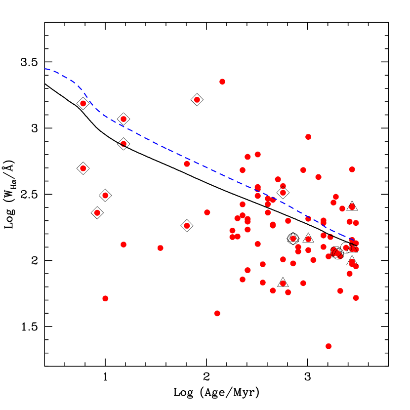
Figure 7.— A comparison of $\rm H\alpha$ equivalent width and age from the SED modeling. The lines show the predicted $W_{\rm H\alpha}$ as a function of age for constant star formation, from Starburst99 models with solar (solid black line) and 0.4 solar (dashed blue line) metallicity. The large scatter of the data with respect to the models is probably caused by variations in the SFR as well as observational uncertainties. Symbols are as in Figure 4.

For simple star formation histories, the evolution of $W_{\rm H\alpha}$ with galaxy age can be predicted with models of stellar evolution and population synthesis. The solid black line in Figure 7 is the theoretically predicted dependence of $W_{\rm H\alpha}$ on age, from a Starburst99 (Leitherer et al. 1999) model with constant star formation, solar metallicity, and a Kroupa (2001) IMF, which gives very similar results to the Chabrier IMF we employ; the dashed blue line is the same, but for $Z=0.4Z_{\odot}$ (as discussed above, metal-rich galaxies are observed to produce less $\rm H\alpha$ luminosity for a given SFR than galaxies of lower metallicity). There is general agreement between the models and the data, but with a large amount of scatter. The equivalent width is a comparison of two quantities with very different timescales; the light from the stellar continuum generally increases over time, while the $\rm H\alpha$ flux may vary stochastically on a much shorter timescale, in response to mergers, feedback, or accretion events. The scatter in the data with respect to the models is $\sim 0.5$ dex, which can be accounted for by a factor of $\sim 2$ change in the current star formation rate with respect to the past average (because a change in the $\rm H\alpha$ flux also affects the inferred continuum flux through the subtraction of $\rm H\alpha$, the equivalent width can change by a larger factor than the star formation rate). A factor of $\sim 2$ is also the typical uncertainty in the star formation rate of individual objects.

The relative extinction of the nebular lines and stellar continuum probably also affects the results here. As mentioned above in the discussion of the star formation rates, we have not used the Calzetti et al. (2000) prescription of $E(B-V)_{\rm stellar}=0.4E(B-V)_{\rm neb}$ for the extinction corrections because doing so results in a significant overestimate of the SFR_Hα with respect to the SFRs from the UV continuum and our models (if we have overestimated the typical aperture correction, then there is room for additional nebular line extinction). Applying this additional extinction correction results in a typical increase of a factor of $\sim 3$ in $W_{\rm H\alpha}$; as can be seen in Figure 7, the mean value of $W_{\rm H\alpha}$ is somewhat below the CSF predictions at a given age, but not usually by a factor of three. It is possible that the HII regions do suffer some smaller amount of additional extinction, however, and this may explain the larger number of objects in our sample that fall below the predictions. This should be more significant for the older objects, as the stars in young galaxies have not had as much time to migrate away from the dusty regions in which they form. It appears from Figure 7, however, that it is the youngest objects that have systematically lower equivalent widths than predicted by the models. These are also the objects for which $W_{\rm H\alpha}$ is the most uncertain, however. The typical uncertainty in $W_{\rm H\alpha}$ is $\sim 40$%, but this approaches $\sim 100$% for the galaxies in which the $\rm H\alpha$ flux makes up most of the $K$-band light; comparisons of ages and equivalent widths should be regarded as highly uncertain in this regime. We also note that the most anomalous point, in the lower left corner, corresponds to Q1700-BX681, which is not well fit by any model SED and therefore has a very uncertain age. As mentioned above, we may have somewhat underestimated the ages of the youngest objects in general, as the ages cannot be significantly less than the dynamical timescale $t_{\rm dyn}\sim 80$ Myr.

Nothing in these results contradicts the hypothesis that the current star formation rate is generally representative of the past average for most of the sample, although stochastic variations are likely. We are not able to strongly discriminate between star formation histories, however; a shallowly declining star formation history would also result in equivalent widths somewhat below the CSF predictions, and this is likely to be an additional factor for some of the objects in the sample, particularly the oldest and most massive. Extrapolating forward in time, the star formation rates of the galaxies in our sample will certainly decline as they lose their gas to star formation or winds; by $z\sim 1$ their clustering properties will best match those of the early-type galaxies in the DEEP2 survey (Adelberger et al. 2005), suggesting that star formation will be largely completed within the next $\sim 3$ Gyr.

6. Summary and Discussion

We have used the $\rm H\alpha$ and UV luminosities of a sample of 114 galaxies at $z\sim 2$ in order to estimate their star formation rates. Using stellar masses and ages determined through population synthesis modeling, we have assessed the star formation properties as a function of stellar mass and age. Our main conclusions are as follows:

1. The sample has a mean star formation rate from extinction-corrected $\rm H\alpha$ luminosity $\langle\rm SFR_{\rm H\alpha}\rangle=31$ $\rm M_{\odot}\;{\rm yr}^{-1}$. The average extinction-corrected UV SFR is $\langle\rm SFR_{UV}\rangle=29$ $\rm M_{\odot}\;{\rm yr}^{-1}$. SFRs range from $\sim 7$ to $\gtrsim 200$ $\rm M_{\odot}\;{\rm yr}^{-1}$, and the average $\rm H\alpha$ SFRs are in excellent agreement with those determined from X-ray, radio, and mid-IR data. The good agreement between the indicators implies that the UV luminosity is attenuated by an typical factor of $\sim 4.5$, while the $\rm H\alpha$ luminosity is attenuated by a factor of $\sim 1.7$ on average. UV attenuation ranges from none to a factor of $\gtrsim 100$, and $\rm H\alpha$ attenuation from none to a factor of $\sim 5$.

2. Star formation rate and $K$ magnitude show significant (4.3$\sigma$) correlation, with the brightest, $K_{s}<20$ galaxies having $\langle\rm SFR_{\rm H\alpha}\rangle\sim 60$ $\rm M_{\odot}\;{\rm yr}^{-1}$. The correlation between SFR and $K$ magnitude is significantly stronger than the correlation between SFR and stellar mass, probably because the rest-frame optical light is strongly affected by current star formation as well as the formed stellar mass.

3. All galaxies in the sample have SFRs per unit area $\Sigma_{\rm SFR}$ in the range observed in local starbursts. All are also above the threshold $\Sigma_{\rm SFR}\geq 0.1$ $\rm M_{\odot}$ yr^-1 kpc^-2 , above which galactic-scale outflows are observed to be ubiquitous in the local universe.

4. We compare the instantaneous SFRs and the past average SFRs as inferred from the ages and stellar masses, finding that for most of the sample, the current SFR appears to be an adequate representation of the past average. There is some evidence that the most massive galaxies ($M_{\star}>10^{11}$ $\rm M_{\odot}$) have had higher SFRs in the past. Both of these conditions can be met by an exponentially declining star formation rate with $\tau=1$–2 Gyr.

It is worth emphasizing the good overall agreement between SFRs determined from $\rm H\alpha$, the UV continuum, X-rays, and radio and mid-IR observations. All of these diagnostics indicate the same average SFR for the sample, and the dispersion between the $\rm H\alpha$ and UV SFRs suggests a typical uncertainty of a factor of $\sim 2$. This result has encouraging implications for the determination of SFRs and the SFR density at high redshift, as it is far easier to obtain UV luminosities for a large sample of galaxies than $\rm H\alpha$ fluxes or deep mid-IR data (and radio and X-ray observations give only the average SFRs of the sample). There has been a widespread perception that the UV luminosity is an unreliable measure of the instantaneous star formation rate, but these results indicate that, for large numbers of high redshift star-forming galaxies, this is not the case.

Another way of stating this result is that the UV slope provides a reasonably accurate indication of extinction in most high redshift star-forming galaxies. This is not a new result; Reddy & Steidel (2004) found that UV luminosities uncorrected for extinction underestimated the bolometric SFRs as determined from X-rays by a factor of $\sim 4.5$–5, in very good agreement with the factor of 4.5 difference we find between the median corrected and uncorrected UV SFRs. Using bolometric luminosities determined from 24µm fluxes, Reddy et al. (2006) find that most star-forming galaxies at $z\sim 2$ follow the local relation between the rest-frame UV slope and dust obscuration. There are important exceptions to this rule, however; the relationship between UV slope and obscuration breaks down for the most luminous galaxies with $L_{\rm bol}\gtrsim 10^{12}$ L_⊙, and young galaxies with ages less than $\sim 100$ Myr also fall away from the relation.

We have also found that, for most of the galaxies in the sample, the current star formation rate appears to be representative of the past average. These results can be usefully compared with those of studies at somewhat lower redshifts; for example, Juneau et al. (2005) use galaxies from the Gemini Deep Deep Survey (GDDS) in the redshift range $0.8<z<2$ to study the dependence of star formation rate on stellar mass. They find that star formation in massive galaxies ($M_{\star}\sim 6-30\times 10^{10}$ $\rm M_{\odot}$) drops steeply after $z\sim 2$ and reaches its low present day value at $z\sim 1$, while the SFR declines more slowly in less massive galaxies. In agreement with this conclusion, we find that all of the galaxies in the current sample are still strongly forming stars, and that the most massive objects are likely to have had higher star formation rates in the past. Erb et al. (2006b) and Reddy et al. (2006) show that these massive galaxies probably have low gas fractions and have thus nearly finished assembling their stellar mass. More generally, the clustering properties of the $z\sim 2$ galaxies (Adelberger et al. 2005) indicate that they will become early-type galaxies with little current star formation by $z\sim 1$.

Table 1Star Formation Rates

					Uncorrected	Corrected			Uncorrected	Corrected
Object	$z_{\rm H\alpha}$	$E(B-V)$	$F_{\rm H\alpha}$	$L_{\rm H\alpha}$	SFRHα	SFRHα	$m_{1500}$	${\rm Log}(L_{1500})$	SFRUV	SFRUV	SFRfit	$W_{\rm H\alpha}$
CDFb-BN88	2.2615	0.149	2.6	1.0	9	14	23.43	29.27	14	60	…	…
HDF-BX1055	2.4899	0.103	2.6	1.3	11	15	24.33	28.98	8	21	4	116
HDF-BX1084	2.4403	0.120	7.3	3.4	30	44	23.5	29.30	16	51	…	…
HDF-BX1085	2.2407	0.171	1.1	0.4	4	6	24.83	28.70	4	20	…	…
HDF-BX1086	2.4435	0.196	1.8	0.8	7	14	25.05	28.68	4	26	…	…
HDF-BX1277	2.2713	0.095	5.3	2.1	18	25	24.01	29.04	8	21	…	…
HDF-BX1303	2.3003	0.100	2.6	1.0	9	12	24.83	28.72	4	11	15	308
HDF-BX1311	2.4843	0.105	8.0	3.9	34	48	23.5	29.31	16	46	7	101
HDF-BX1322	2.4443	0.085	2.0	0.9	8	11	24.03	29.09	10	22	34	197
HDF-BX1332	2.2136	0.290	4.4	1.6	14	35	23.96	29.04	8	135	19	68
HDF-BX1368	2.4407	0.160	8.8	4.1	36	59	24.09	29.06	9	44	159	132
HDF-BX1376	2.4294	0.070	2.2	1.0	9	11	24.49	28.90	6	12	37	266
HDF-BX1388	2.0317	0.265	5.8	1.8	15	34	24.82	28.63	3	38	9	265
HDF-BX1397	2.1328	0.150	5.3	1.8	16	25	24.26	28.89	6	25	23	90
HDF-BX1409	2.2452	0.290	8.5	3.2	29	69	25.15	28.57	3	47	17	207
HDF-BX1439	2.1865	0.175	8.8	3.2	28	48	24.16	28.95	7	36	27	145
HDF-BX1479	2.3745	0.110	2.5	1.1	10	14	24.55	28.86	6	16	21	107
HDF-BX1564	2.2225	0.065	8.6	3.2	28	34	23.55	29.21	13	23	13	126
HDF-BX1567	2.2256	0.050	4.0	1.5	13	15	23.68	29.15	11	18	9	93
HDF-BX305	2.4839	0.285	4.2	2.1	18	43	25.07	28.68	4	65	5	72
HDF-BMZ1156	2.2151	0.000	5.4	2.0	18	18	24.61	28.78	5	5	53	67
Q0201-B13	2.1663	0.003	2.4	0.8	7	8	23.36	29.26	14	15	…	…
Q1307-BM1163	1.4105	0.178	28.7	3.5	31	53	22.21	29.38	19	99	…	…
Q1623-BX151	2.4393	0.059	3.5	1.6	14	17	24.74	28.80	5	9	…	…
Q1623-BX214	2.4700	0.182	5.3	2.6	23	39	24.45	28.92	7	40	…	…
Q1623-BX215	2.1814	0.134	4.8	1.7	15	22	24.71	28.73	4	15	…	…
Q1623-BX252	2.3367	0.031	1.2	0.5	4	5	25.13	28.61	3	4	…	…
Q1623-BX274	2.4100	0.119	9.5	4.3	38	54	23.48	29.29	15	50	…	…
Q1623-BX344	2.4224	0.189	17.1	7.9	69	123	24.81	28.77	5	30	…	…
Q1623-BX366	2.4204	0.200	7.9	3.6	32	58	24.25	28.99	8	55	…	…
Q1623-BX376	2.4085	0.175	5.3	2.4	21	36	23.55	29.27	14	81	80	183
Q1623-BX428	2.0538	0.000	2.7	0.8	7	7	24.08	28.93	7	7	1	84
Q1623-BX429	2.0160	0.120	5.1	1.5	13	19	23.75	29.05	9	26	23	219
Q1623-BX432	2.1817	0.060	5.4	1.9	17	20	24.68	28.74	4	8	6	427
Q1623-BX447	2.1481	0.050	5.6	1.9	17	20	24.65	28.74	4	7	5	154
Q1623-BX449	2.4185	0.110	3.5	1.6	14	20	25.06	28.67	4	11	9	196
Q1623-BX452	2.0595	0.195	4.4	1.4	12	22	24.93	28.60	3	19	14	121
Q1623-BX453	2.1816	0.275	13.8	4.9	43	100	23.86	29.07	9	123	107	187
Q1623-BX455	2.4074	0.265	18.8	8.6	75	169	25.15	28.63	3	45	58	1172
Q1623-BX458	2.4194	0.165	4.3	2.0	17	29	23.69	29.21	13	65	55	102
Q1623-BX472	2.1142	0.130	3.9	1.3	11	17	24.74	28.69	4	13	11	135
Q1623-BX502	2.1558	0.220	13.2	4.6	40	79	24.57	28.77	5	37	72	1536
Q1623-BX511	2.2421	0.235	3.4	1.3	11	23	25.79	28.32	2	15	13	325
Q1623-BX513	2.2473	0.145	3.3	1.3	11	17	23.51	29.23	13	53	46	59
Q1623-BX516	2.4236	0.145	5.2	2.4	21	33	24.24	28.99	8	32	28	112
Q1623-BX522	2.4757	0.180	2.8	1.4	12	21	24.81	28.78	5	28	24	79
Q1623-BX528	2.2682	0.175	7.7	3.0	27	46	23.81	29.12	10	55	44	94
Q1623-BX543	2.5211	0.305	8.6	4.4	39	98	23.55	29.30	16	336	528	229
Q1623-BX586	2.1045	0.195	5.1	1.7	15	27	24.9	28.62	3	20	17	192
Q1623-BX599	2.3304	0.125	18.1	7.6	67	98	23.66	29.20	12	42	35	303
Q1623-BX663	2.4333	0.135	8.2	3.8	33	50	24.38	28.94	7	26	21	112
Q1623-MD107	2.5373	0.060	3.7	1.9	17	20	25.47	28.54	3	5	4	858
Q1623-MD66	2.1075	0.235	19.7	6.5	57	116	24.32	28.86	6	50	43	482
Q1700-BX490	2.39597	0.285	17.7	8.0	70	166	23.24	29.39	19	313	448	310
Q1700-BX505	2.3089	0.270	3.6	1.5	13	29	25.62	28.41	2	27	20	121
Q1700-BX523	2.4756	0.260	4.7	2.3	20	44	24.97	28.72	4	55	42	171
Q1700-BX530	1.94294	0.045	12.2	3.3	29	33	23.26	29.22	13	19	6	208
Q1700-BX536	1.9780	0.115	11.3	3.2	28	40	23.21	29.25	14	40	15	150
Q1700-BX561	2.4332	0.130	1.9	0.9	8	11	24.84	28.76	4	16	10	22
Q1700-BX581	2.4022	0.215	4.0	1.8	16	30	24.15	29.02	8	69	70	124
Q1700-BX681	1.73959	0.315	6.3	1.3	11	30	22.23	29.54	27	427	628	52
Q1700-BX691	2.1895	0.125	7.7	2.8	24	36	25.55	28.39	2	6	5	257
Q1700-BX717	2.4353	0.090	3.8	1.8	16	20	24.98	28.70	4	10	8	410
Q1700-BX759	2.4213	0.230	1.3	0.6	5	11	24.79	28.77	5	45	37	57
Q1700-BX794	2.2473	0.130	6.8	2.6	23	34	23.95	29.05	9	31	25	183
Q1700-BX917	2.3069	0.040	7.4	3.0	27	30	24.71	28.77	5	7	4	117
Q1700-MD69	2.2883	0.275	7.5	3.0	26	61	25.22	28.56	3	40	31	122
Q1700-MD94	2.33624	0.500	12.9	5.4	48	219	25.66	28.40	2	253	213	146
Q1700-MD103	2.3148	0.305	8.2	3.4	30	76	24.69	28.78	5	90	65	120
Q1700-MD109	2.2942	0.175	2.8	1.1	10	17	25.72	28.36	2	10	8	246
Q1700-MD154	2.62911	0.335	4.1	2.3	20	56	23.96	29.17	12	359	347	40
Q1700-MD174	2.3423	0.195	8.9	3.8	33	60	24.88	28.71	4	27	24	125
Q2343-BM133	1.47744	0.115	28.7	3.9	35	49	22.78	29.19	12	36	35	2245
Q2343-BM181	1.4951	0.134	3.4	0.5	4	6	25.18	28.24	1	5	…	…
Q2343-BX163	2.12132	0.050	2.2	0.7	6	7	24.06	28.97	7	12	9	127
Q2343-BX169	2.20939	0.125	4.7	1.7	15	22	23.3	29.30	16	51	46	152
Q2343-BX182	2.2879	0.100	2.4	1.0	8	11	23.88	29.10	10	26	23	168
Q2343-BX236	2.43475	0.085	3.1	1.4	13	16	24.42	28.93	7	15	13	150
Q2343-BX336	2.54387	0.210	4.3	2.2	20	38	24.31	29.00	8	66	58	133
Q2343-BX341	2.5749	0.210	4.0	2.1	19	36	24.59	28.90	6	52	50	231
Q2343-BX378	2.04407	0.165	4.5	1.4	12	20	25.06	28.54	3	12	11	606
Q2343-BX389	2.17156	0.250	12.0	4.2	37	80	25.13	28.56	3	30	22	253
Q2343-BX390	2.2313	0.150	4.9	1.9	16	26	24.6	28.79	5	20	17	293
Q2343-BX391	2.17403	0.195	4.2	1.5	13	24	24.51	28.80	5	31	25	537
Q2343-BX418	2.3052	0.035	8.0	3.3	29	32	23.94	29.08	9	13	12	1639
Q2343-BX429	2.1751	0.185	4.8	1.7	15	27	25.42	28.44	2	12	12	632
Q2343-BX435	2.1119	0.225	8.1	2.7	24	47	24.61	28.74	4	35	30	200
Q2343-BX436	2.3277	0.070	7.2	3.0	26	33	23.19	29.38	19	37	33	345
Q2343-BX442	2.1760	0.225	7.2	2.5	22	44	24.48	28.82	5	43	25	98
Q2343-BX461	2.5662	0.250	7.0	3.7	33	70	24.84	28.80	5	62	86	760
Q2343-BX474	2.2257	0.215	5.0	1.9	16	32	24.73	28.73	4	33	26	133
Q2343-BX480	2.2313	0.165	3.0	1.1	10	16	24.06	29.00	8	38	33	67
Q2343-BX493	2.33964	0.255	5.3	2.2	20	43	23.91	29.10	10	118	220	497
Q2343-BX513	2.10919	0.135	10.1	3.3	29	44	24.13	28.93	7	24	20	192
Q2343-BX529	2.1129	0.145	3.5	1.2	10	16	24.62	28.74	4	17	14	230
Q2343-BX537	2.3396	0.130	5.2	2.2	19	29	24.67	28.80	5	17	15	365
Q2343-BX587	2.2430	0.180	5.5	2.1	19	32	23.79	29.12	10	57	49	95
Q2343-BX599	2.01156	0.100	4.5	1.3	12	16	23.6	29.11	10	25	21	107
Q2343-BX601	2.3769	0.125	7.4	3.3	29	42	23.7	29.20	12	42	36	199
Q2343-BX610	2.2094	0.155	8.1	3.0	26	42	23.92	29.05	9	38	32	59
Q2343-BX660	2.1735	0.010	9.4	3.3	29	30	24.27	28.90	6	7	5	488
Q2343-MD59	2.01159	0.200	2.9	0.8	7	14	24.99	28.55	3	18	11	52
Q2343-MD62	2.17524	0.150	2.3	0.8	7	11	25.5	28.41	2	8	7	143
Q2343-MD80	2.0138	0.020	3.2	0.9	8	9	24.81	28.63	3	4	1	206
Q2346-BX120	2.2664	0.005	5.3	2.1	18	19	25.1	28.60	3	3	…	…
Q2346-BX220	1.9677	0.055	10.3	2.9	25	30	23.86	28.99	8	13	4	482
Q2346-BX244	1.6465	0.300	5.4	1.0	9	21	23.49	29.00	8	149	…	…
Q2346-BX404	2.0282	0.095	13.9	4.2	36	49	23.57	29.13	10	25	22	273
Q2346-BX405	2.0300	0.010	14.0	4.2	37	38	23.44	29.18	12	13	7	358
Q2346-BX416	2.2404	0.195	12.1	4.6	41	73	23.89	29.08	9	60	55	287
Q2346-BX482	2.2569	0.112	11.2	4.4	38	54	23.54	29.22	13	38	…	…
SSA22a-MD41	2.1713	0.096	7.9	2.8	25	33	23.5	29.21	13	31	…	…
West-BM115	1.6065	0.225	5.9	1.0	9	17	24.05	28.75	4	40	…	…
West-BX600	2.1607	0.047	6.3	2.2	19	22	24.04	28.99	8	12	…	…

References

- Adelberger et al. (2005) Adelberger, K. L., Steidel, C. C., Pettini, M., Shapley, A. E., Reddy, N. A., & Erb, D. K. 2005, ApJ, 619, 697
- Brinchmann et al. (2004) Brinchmann, J., Charlot, S., White, S. D. M., Tremonti, C., Kauffmann, G., Heckman, T., & Brinkmann, J. 2004, MNRAS, 351, 1151
- Bruzual & Charlot (2003) Bruzual, G. & Charlot, S. 2003, MNRAS, 344, 1000
- Calzetti et al. (2000) Calzetti, D., Armus, L., Bohlin, R. C., Kinney, A. L., Koornneef, J., & Storchi-Bergmann, T. 2000, ApJ, 533, 682
- Chabrier (2003) Chabrier, G. 2003, PASP, 115, 763
- Chapman et al. (2005) Chapman, S. C., Blain, A. W., Smail, I., & Ivison, R. J. 2005, ApJ, 622, 772
- Cimatti et al. (2002) Cimatti, A., Daddi, E., Mignoli, M., Pozzetti, L., Renzini, A., Zamorani, G., Broadhurst, T., Fontana, A., Saracco, P., Poli, F., Cristiani, S., D’Odorico, S., Giallongo, E., Gilmozzi, R., & Menci, N. 2002, A&A, 381, L68
- Daddi et al. (2004) Daddi, E., Cimatti, A., Renzini, A., Fontana, A., Mignoli, M., Pozzetti, L., Tozzi, P., & Zamorani, G. 2004, ApJ, 617, 746
- Dickinson et al. (2003) Dickinson, M., Papovich, C., Ferguson, H. C., & Budavári, T. 2003, ApJ, 587, 25
- Erb et al. (2006a) Erb, D. K., Shapley, A. E., Pettini, M., Steidel, C. C., Reddy, N. A., & Adelberger, K. L. 2006a, ApJ, in press, astro-ph/0602473
- Erb et al. (2003) Erb, D. K., Shapley, A. E., Steidel, C. C., Pettini, M., Adelberger, K. L., Hunt, M. P., Moorwood, A. F. M., & Cuby, J. 2003, ApJ, 591, 101
- Erb et al. (2006b) Erb, D. K., Steidel, C. C., Shapley, A. E., Pettini , M., Reddy, N. A., & Adelberger, K. L. 2006b, ApJ, in press, astro-ph/0604041
- Franx et al. (2003) Franx, M., Labbé, I., Rudnick, G., van Dokkum, P. G., Daddi, E., Förster Schreiber, N. M., Moorwood, A., Rix, H., Röttgering, H., van de Wel, A., van der Werf, P., & van Starkenburg, L. 2003, ApJ, 587, L79
- Heavens et al. (2004) Heavens, A., Panter, B., Jimenez, R., & Dunlop, J. 2004, Nature, 428, 625
- Heckman (2002) Heckman, T. M. 2002, in ASP Conf. Ser. 254: Extragalactic Gas at Low Redshift, 292–+
- Hopkins et al. (2003) Hopkins, A. M., Miller, C. J., Nichol, R. C., Connolly, A. J., Bernardi, M., Gómez, P. L., Goto, T., Tremonti, C. A., Brinkmann, J., Ivezić, Ž., & Lamb, D. Q. 2003, ApJ, 599, 971
- Juneau et al. (2005) Juneau, S., Glazebrook, K., Crampton, D., McCarthy, P. J., Savaglio, S., Abraham, R., Carlberg, R. G., Chen, H., Le Borgne, D., Marzke, R. O., Roth, K., Jørgensen, I., Hook, I., & Murowinski, R. 2005, ApJ, 619, L135
- Kennicutt (1998a) Kennicutt, R. C. 1998a, ARA&A, 36, 189
- Kennicutt (1998b) —. 1998b, ApJ, 498, 541
- Kroupa (2001) Kroupa, P. 2001, MNRAS, 322, 231
- Leitherer et al. (1999) Leitherer, C., Schaerer, D., Goldader, J. D., Delgado, R. M. G., Robert, C., Kune, D. F., de Mello, D. F., Devost, D., & Heckman, T. M. 1999, ApJS, 123, 3
- McLean et al. (1998) McLean, I. S., Becklin, E. E., Bendiksen, O., Brims, G., Canfield, J., Figer, D. F., Graham, J. R., Hare, J., Lacayanga, F., Larkin, J. E., Larson, S. B., Levenson, N., Magnone, N., Teplitz, H., & Wong, W. 1998, in Proc. SPIE Vol. 3354, p. 566-578, Infrared Astronomical Instrumentation, Albert M. Fowler; Ed., Vol. 3354, 566–578
- Papovich et al. (2001) Papovich, C., Dickinson, M., & Ferguson, H. C. 2001, ApJ, 559, 620
- Papovich et al. (2005) Papovich, C., Moustakas, L. A., Dickinson, M., Le Floc’h, E., Rieke, G. H., Daddi, E., Alexander, D. M., Bauer, F., Brandt, W. N., Dahlen, T., Egami, E., Eisenhardt, P., Elbaz, D., Ferguson, H. C., Giavalisco, M., Lucas, R. A., Mobasher, B., Perez-Gonzalez, P. G., Stutz, A., Rieke, M. J., & Yan, H. 2005, ApJ, in press, astro-ph/0511289
- Reddy et al. (2005) Reddy, N. A., Erb, D. K., Steidel, C. C., Shapley, A. E., Adelberger, K. L., & Pettini, M. 2005, ApJ, 633, 748
- Reddy & Steidel (2004) Reddy, N. A. & Steidel, C. C. 2004, ApJ, 603, L13
- Reddy et al. (2006) Reddy, N. A., Steidel, C. C., Fadda, D., Yan, L., Pettini, M., Shapley, A. E., Erb, D. K., & Adelberger, K. L. 2006, ApJ, in press, astro-ph/0602596
- Rudnick et al. (2003) Rudnick, G., Rix, H.-W., Franx, M., Labbé, I., Blanton, M., Daddi, E., Förster Schreiber, N. M., Moorwood, A., Röttgering, H., Trujillo, I., van de Wel, A., van der Werf, P., van Dokkum, P. G., & van Starkenburg, L. 2003, ApJ, 599, 847
- Salpeter (1955) Salpeter, E. E. 1955, ApJ, 121, 161
- Shapley et al. (2004) Shapley, A. E., Erb, D. K., Pettini, M., Steidel, C. C., & Adelberger, K. L. 2004, ApJ, 612, 108
- Shapley et al. (2001) Shapley, A. E., Steidel, C. C., Adelberger, K. L., Dickinson, M., Giavalisco, M., & Pettini, M. 2001, ApJ, 562, 95
- Shapley et al. (2005) Shapley, A. E., Steidel, C. C., Erb, D. K., Reddy, N. A., Adelberger, K. L., Pettini, M., Barmby, P., & Huang, J. 2005, ApJ, 626, 698
- Steidel et al. (2005) Steidel, C. C., Adelberger, K. L., Shapley, A. E., Erb, D. K., Reddy, N. A., & Pettini, M. 2005, ApJ, 626, 44
- Steidel et al. (2004) Steidel, C. C., Shapley, A. E., Pettini, M., Adelberger, K. L., Erb, D. K., Reddy, N. A., & Hunt, M. P. 2004, ApJ, 604, 534
- Swinbank et al. (2004) Swinbank, A. M., Smail, I., Chapman, S. C., Blain, A. W., Ivison, R. J., & Keel, W. C. 2004, ApJ, 617, 64
- van Dokkum et al. (2004) van Dokkum, P. G., Franx, M., Förster Schreiber, N. M., Illingworth, G. D., Daddi, E., Knudsen, K. K., Labbé, I., Moorwood, A., Rix, H., Röttgering, H., Rudnick, G., Trujillo, I., van der Werf, P., van der Wel, A., van Starkenburg, L., & Wuyts, S. 2004, ApJ, 611, 703
- Wilson et al. (2003) Wilson, J. C., Eikenberry, S. S., Henderson, C. P., Hayward, T. L., Carson, J. C., Pirger, B., Barry, D. J., Brandl, B. R., Houck, J. R., Fitzgerald, G. J., & Stolberg, T. M. 2003, in Instrument Design and Performance for Optical/Infrared Ground-based Telescopes. Edited by Iye, Masanori; Moorwood, Alan F. M. Proceedings of the SPIE, Volume 4841, pp. 451-458 (2003)., 451–458