A numerical study of non-gaussianity in the curvaton scenario

Abstract

We study the curvaton scenario using gauge-invariant second order perturbation theory and solving the governing equations numerically. Focusing on large scales we calculate the non-linearity parameter $f_{\rm{NL}}$ in the two-fluid curvaton model and compare our results with previous analytical studies employing the sudden decay approximation. We find good agreement of the two approaches for large curvaton energy densities at curvaton decay, $\Omega_{\sigma\rm{dec}}$, but significant differences of up to $10\%$ for small $\Omega_{\sigma\rm{dec}}$.

I Introduction

The third year WMAP data release WMAP has confirmed beautifully the cosmological standard model of structure formation: during inflation fluctuations in the scalar fields are stretched to super-horizon scales and later on source the Cosmic Microwave Background (CMB) anisotropies and the large scale structure. In the standard inflation models the scalar field responsible for the accelerated expansion of the universe, the inflaton, also provides these fluctuations LLBook . Recently a related but different scenario has become become popular: the curvaton paradigm curvaton ; MT ; Enqvist ; LUW ; MWU ; Lyth:2003dt ; GMW ; Enqvist:2005pg ; Linde2005 ; Lyth2006 . Here the fluctuations are not generated by the inflaton, but by a different scalar field, the curvaton.

A powerful tool to differentiate between different models of the early universe is second order perturbation theory Mukhanov ; Bruni ; Maldacena ; Acquaviva ; Nakamura ; Noh ; Bartolo:2001cw ; Bernardeau:2002jy ; Bernardeau:2002jf ; MW2004 ; Bartolo2003 ; Bartolo:2004if ; Bartolo:2004ty ; Enqvist:2004bk ; RiSh ; Rigopoulos:2004ba ; Bartolo:JCAP ; Tomita:2005et ; Lyth:2005du ; Seery:2005gb ; M2005 . It allows the accurate calculation of higher order statistics such as the primordial bispectrum and the non-linearity parameter $f_{\rm{NL}}$. Instead of using cosmological perturbation theory at second order, the $\Delta N$-formalism SB ; SaSt95 ; SaTa ; LMS ; Lyth:2005fi ; LaVe has proved useful to study non-gaussianity and calculate $f_{\rm{NL}}$.

Bartolo et al. Bartolo2003 studied the curvaton model at second order using cosmological perturbation theory, and Lyth and Rodriguez used the $\Delta N$-formalism to calculate the non-linearity parameter $f_{\rm{NL}}$ in this scenario. However, both studies used the sudden decay approximation. Here we go beyond sudden decay, using second order gauge-invariant perturbation theory and solve the ensuing equations numerically.

We consider scalar perturbations up to and including second order and assume a flat Friedmann-Robertson-Walker (FRW) background spacetime. We work on large scales (compared to the horizon size), which allows us to neglect gradient terms.

The outline of the paper is as follows. In the next section we give the governing equations up to second order and define the gauge-invariant variables we are using. We specify in Section III the two-fluid curvaton model we are studying and apply the equations of Section II. In Section IV we take a small detour from perturbation theory and compare our perturbative approach to the $\Delta N$ formalism. After defining the non-linearity parameter $f_{\rm{NL}}$ we present numerical solutions in Section V and compare our numerical results to the sudden decay approximation. The governing equations without any gauge restrictions are given in the appendix.

II Governing equations

In this section we give the governing equations for a system of multiple interacting fluids on large scales, allowing for scalar perturbations up to second order, following closely the treatment of Refs. MW2004 and MW2005 .

The covariant Einstein equations are given by

$$G_{\mu\nu}=8\pi G\;T_{\mu\nu}\,,$$ (1)

where $G_{\mu\nu}$ is the Einstein tensor, $T_{\mu\nu}$ is the total energy-momentum tensor, and $G$ is Newton’s constant. Through the Bianchi identities, the field equations (1) imply the local conservation of the total energy and momentum,

$$\nabla_{\mu}T^{\mu\nu}=0\,.$$ (2)

In the multiple fluid case the total energy-momentum tensor is the sum of the energy-momentum tensors of the individual fluids

$$T^{\mu\nu}=\sum_{\alpha}T^{\mu\nu}_{(\alpha)}\,.$$ (3)

For each fluid we define the local energy-momentum transfer 4-vector $Q^{\nu}_{(\alpha)}$ through the relation

$$\nabla_{\mu}T^{\mu\nu}_{(\alpha)}=Q^{\nu}_{(\alpha)}\,,$$ (4)

where energy-momentum is locally conserved for $Q^{\nu}_{(\alpha)}=0$, i.e. only for non-interacting fluids. Equations (2) and (4) imply the constraint

$$\sum_{\alpha}Q^{\nu}_{(\alpha)}=0\,.$$ (5)

We split scalar perturbations into background, first, and second order quantities according to,

$$\rho(x^{\mu})\equiv\rho_{0}(t)+\delta\rho_{1}(x^{\mu})+\frac{1}{2}\delta\rho_{2}(x^{\mu})\,,$$ (6)

using here the total energy density as an example.

The line element on large scales is given by

$$ds^{2}=-\left[1+2\left(\phi_{1}+\frac{1}{2}\phi_{2}\right)\right]dt^{2}+a^{2}\left[1-2\left(\psi_{1}-\frac{1}{2}\psi_{2}\right)\right]\delta_{ij}dx^{i}dx^{j}\,,$$ (7)

where $a=a(t)$ is the scale factor, $\phi_{1}$ and $\phi_{2}$ are the lapse functions at first and second order, respectively, and $\psi_{1}$ and $\psi_{2}$ the curvature perturbations.

Following Refs. KS ; MW2005 we split the energy-momentum transfer 4-vector using the total fluid velocity $u^{\mu}$ as

$$Q^{\mu}_{(\alpha)}\equiv Q_{(\alpha)}u^{\mu}+f^{\mu}_{(\alpha)}\,,$$ (8)

where $Q_{(\alpha)}$ is the energy transfer rate and $f^{\mu}_{(\alpha)}$ the momentum transfer rate, subject to the condition $u_{\mu}f^{\mu}_{(\alpha)}=0$.

On large scales the only non-zero component of the 4-velocity is

$$u_{0} = -\left[1+\phi_{1}+\frac{1}{2}\phi_{2}-\frac{1}{2}\phi_{1}^{2}\right]\,,$$ (9)

subject to the constraint $u_{\mu}u^{\mu}=-1$. We then find the only non-zero component of the energy transfer 4-vector on large scales to be

$$Q_{0(\alpha)}=-Q_{0\alpha}\left(1+\phi_{1}+\frac{1}{2}\phi_{2}-\frac{1}{2}\phi_{1}^{2}\right)-\delta Q_{1\alpha}\left(1+\phi_{1}\right)-\delta Q_{2\alpha}\,,$$ (11)

where $Q_{0\alpha}$, $\delta Q_{1\alpha}$, and $\delta Q_{2\alpha}$ are the energy transfer to the $\alpha$-fluid in the background, at first and at second order, respectively.

II.1 Background

Energy conservation for the $\alpha$-fluid in the background is given from Eq. (4) as

$$\dot{\rho}_{0\alpha}=-3H\left(\rho_{0\alpha}+P_{0\alpha}\right)+Q_{0\alpha}\,,$$ (12)

where $H=\dot{a}/a$ is the Hubble parameter, and $\rho_{0\alpha}$ and $P_{0\alpha}$ are the energy density and the pressure, respectively, of the $\alpha$-fluid. Total energy conservation is then given by summing over the individual fluids and using Eq. (5) as

$$\dot{\rho}_{0}=-3H\left(\rho_{0}+P_{0}\right)\,,$$ (13)

where $\rho_{0}=\sum_{\alpha}\rho_{0\alpha}$.

The Friedmann constraint is given from the $0-0$ component Eq. (1) as

$$H^{2}=\frac{8\pi G}{3}\rho_{0}\,.$$ (14)

II.2 First order perturbations

We now give the governing equations on large scales at first order in the perturbations in the flat gauge, denoting quantities evaluated in this gauge by a “tilde”. The governing equations in an arbitrary gauge are given in appendix A.1.1.

The energy conservation equation for the $\alpha$-fluid at first order is given from Eq. (4) on large scales as

$$\dot{\widetilde{\delta\rho_{1\alpha}}}+3H\left(\widetilde{\delta\rho_{1\alpha}}+\widetilde{\delta P_{1\alpha}}\right)-Q_{0\alpha}\widetilde{\phi_{1}}-\widetilde{\delta Q_{1\alpha}}=0\,.$$ (15)

The total energy density perturbation is related to the individual fluid densities, and similarly for the pressure perturbations, by

$$\widetilde{\delta\rho_{1}} \equiv \sum_{\alpha}\widetilde{\delta\rho_{1\alpha}}\,,\qquad\widetilde{\delta P_{1}}\equiv\sum_{\alpha}\widetilde{\delta P_{1\alpha}}\,,$$ (16)

and we get, using the constraint Eq. (5), from Eq. (15) the evolution equation for the total energy density perturbation

$$\dot{\widetilde{\delta\rho_{1}}}+3H\left(\widetilde{\delta\rho_{1}}+\widetilde{\delta P_{1}}\right)=0\,.$$ (17)

The $0-0$ Einstein equation on flat slices is, using Eq. (1) and the background Friedmann constraint (14), given by

$$\widetilde{\phi}_{1}=-\frac{1}{2}\frac{\widetilde{\delta\rho_{1}}}{\rho_{0}}\,.$$ (18)

The curvature perturbation on uniform $\alpha$ fluid energy density hyper-surfaces at first order is given by WMLL

$$\zeta_{1\alpha}=-H\frac{\delta\rho_{1\alpha}}{\dot{\rho}_{0\alpha}}\,.$$ (19)

The curvature perturbation on uniform total energy density hyper-surfaces at first order is given by

$$\zeta_{1}=-\frac{H}{\dot{\rho}_{0}}\widetilde{\delta\rho_{1}}\,,$$ (20)

and related to the curvature perturbation on uniform $\alpha$ fluid slices by

$$\zeta_{1}=\sum_{\alpha}\frac{\dot{\rho}_{0\alpha}}{\dot{\rho}_{0}}\zeta_{1\alpha}\,.$$ (21)

As in the background we introduce new variables, the normalised energy densities at first order,

$$\delta\Omega_{1\alpha}\equiv\frac{\widetilde{\delta\rho_{1\alpha}}}{\rho_{0}}\,,$$ (22)

which allow us in combination with choosing the number of e-foldings as a time variable to write the governing equations in the following sections in a particularly compact form.

In terms of the new variables the curvature perturbation on uniform $\alpha$ fluid energy density hyper-surfaces, given in Eq. (19), is simply

$$\zeta_{1\alpha}=-H\frac{\rho_{0}}{\dot{\rho}_{0\alpha}}\delta\Omega_{1\alpha}\,.$$ (23)

II.3 Second order

We now give the governing equations on large scales at second order in the perturbations in the flat gauge, denoting quantities evaluated in this gauge by a “tilde”. The governing equations in an arbitrary gauge are given in appendix A.1.2.

The energy conservation equation for the $\alpha$-fluid at second order is given from Eq. (4) on large scales by

$$\dot{\widetilde{\delta\rho_{2\alpha}}}+3H\left(\widetilde{\delta\rho_{2\alpha}}+\widetilde{\delta P_{2\alpha}}\right)-Q_{0\alpha}\left(\widetilde{\phi_{2}}-{\widetilde{\phi_{1}}}^{2}\right)-\widetilde{\delta Q_{2\alpha}}-2\phi_{1}\widetilde{\delta Q_{1\alpha}}=0\,.$$ (24)

Using Eq. (5) the evolution equation for the total energy density is

$$\dot{\widetilde{\delta\rho_{2}}}+3H\left(\widetilde{\delta\rho_{2}}+\widetilde{\delta P_{2}}\right)=0\,,$$ (25)

where the total density and pressure perturbations are given in terms of the individual fluid ones by

$$\widetilde{\delta\rho_{2}}\equiv\sum_{\alpha}\widetilde{\delta\rho_{2\alpha}}\,,\qquad\widetilde{\delta P_{2}}\equiv\sum_{\alpha}\widetilde{\delta P_{2\alpha}}\,.$$ (26)

The $0-0$ Einstein equation on flat slices is, using Eq. (1) and the background Friedmann constraint (14), given by

$$\widetilde{\phi}_{2}-4\widetilde{\phi_{1}}^{2}=-\frac{1}{2}\frac{\widetilde{\delta\rho_{2}}}{\rho_{0}}\,.$$ (27)

The curvature perturbation at second order in terms of uniform $\alpha$-density perturbations on flat slices is given by MW2004 ; M2005

$$\zeta_{2\alpha}=-\frac{H}{\dot{\rho}_{0\alpha}}\widetilde{\delta\rho_{2\alpha}}+2\frac{H}{{\dot{\rho}_{0\alpha}}^{2}}\dot{\widetilde{\delta\rho_{1\alpha}}}\widetilde{\delta\rho_{1\alpha}}+\frac{H}{{\dot{\rho}_{0\alpha}}^{2}}\left[H\left(5+3c_{\rm{\alpha}}^{2}\right)+\frac{\dot{H}}{H}\frac{Q_{0\alpha}}{\dot{\rho}_{0\alpha}}-\frac{\dot{Q}_{0\alpha}}{\dot{\rho}_{0\alpha}}\right]{\widetilde{\delta\rho_{1\alpha}}}^{2}\,,$$ (28)

where $c_{\rm{\alpha}}^{2}\equiv\dot{P}_{0\alpha}/\dot{\rho}_{0\alpha}$ is the adiabatic sound speed of the $\alpha$-fluid.

The curvature perturbation at second order in terms of the total density perturbations on flat slices is given by MW2004

$$\zeta_{2}=-\frac{H}{\dot{\rho}_{0}}\widetilde{\delta\rho_{2}}+2\frac{H}{{\dot{\rho}_{0}}^{2}}\dot{\widetilde{\delta\rho_{1}}}\widetilde{\delta\rho_{1}}+\frac{H^{2}}{{\dot{\rho}_{0}}^{2}}\left(5+3c_{\rm{s}}^{2}\right){\widetilde{\delta\rho_{1}}}^{2}\,,$$ (29)

where $c_{\rm{s}}^{2}\equiv\dot{P}_{0}/\dot{\rho}_{0}$ is the total adiabatic sound speed related to the individual speeds $c_{\rm{\alpha}}^{2}$ by

$$c_{\rm{s}}^{2}=\sum_{\alpha}\frac{\dot{\rho}_{0\alpha}}{\dot{\rho}_{0}}c_{\rm{\alpha}}^{2}\,.$$ (30)

As at first order we introduce new variables, the normalised energy densities at second order, allowing us to rewrite the governing equations in the following sections in a particularly compact form,

$$\delta\Omega_{2\alpha}\equiv\frac{\widetilde{\delta\rho_{2\alpha}}}{\rho_{0}}\,.$$ (31)

The curvature perturbation $\zeta_{2}$, defined above in Eq. (29), is related to the curvature perturbation employed in the $\Delta N$ formalism (see also LW ), which we denote by $\zeta_{2\rm{SB}}$, by LMS ; Lyth:2005du

$$\zeta_{2\rm{SB}}=\zeta_{2}-2\zeta_{1}^{2}\,.$$ (32)

It was originally introduced by Salopek and Bond SB and employed by Maldacena in studies of non-gaussianity in Ref. Maldacena .

III The model

In this section we specify the curvaton model and apply the governing equations given in the previous section order by order. We model the curvaton as a pressureless fluid curvaton , and hence our system will be governed by the equations of state

$$P_{\sigma}=0\,,\qquad P_{\gamma}=\frac{1}{3}\rho_{\gamma}\,,$$ (33)

where the subscripts “$\sigma$” and “$\gamma$” denote the curvaton and the radiation fluid, respectively. The decay of the curvaton is described by a fixed decay rate, $\Gamma=const$,

$$Q_{\sigma}=-\Gamma\rho_{\sigma}\,,\qquad Q_{\gamma}=\Gamma\rho_{\sigma}\,,$$ (34)

where we used Eq. (5).

III.1 Background

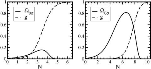
Figure 1: Evolution of the normalised background curvaton density, $\Omega_{0\sigma}$, and the normalised decay rate $g$, as a function of the number of e-foldings, starting with initial density and decay rate $\Omega_{0\sigma}=10^{-2}$ and $\Gamma/H=10^{-3}$, corresponding to $p_{\rm{in}}=0.32$ on the left panel, and on the right panel with $\Gamma/H=10^{-6}$, corresponding to $p_{\rm{in}}=10$.

The background evolution equations are from Eq. (12) and using Eqs. (33) and (34) given by

$$\dot{\rho}_{\sigma} = -3H\rho_{0\sigma}-\Gamma\rho_{0\sigma}\,,$$ (35)

$$\dot{\rho}_{0\gamma} = -4H\rho_{0\gamma}+\Gamma\rho_{0\sigma}\,.$$ (36)

We now change to a new set of variables. First we introduce normalised energy densities in the background,

$$\Omega_{0\alpha}\equiv\frac{\rho_{0\alpha}}{\rho_{0}}\,,$$ (37)

and define the reduced decay rate as

$$g\equiv\frac{\Gamma}{\Gamma+H}\,.$$ (38)

We change the time coordinate from coordinate time $t$ to the number of e-foldings $N\equiv\ln a$, that is $\frac{d}{dt}=H\frac{d}{dN}$. The normalised radiation energy density is then simply given from the Friedmann equation, (14), as $\Omega_{0\gamma}\equiv 1-\Omega_{0\sigma}$ and we get the system of background evolution equations in terms of these new variables

$$\Omega_{0\sigma}^{\prime} = \Omega_{0\sigma}\left(1-\Omega_{0\sigma}-\frac{g}{1-g}\right)\,,$$ (39)

$$g^{\prime} = \frac{1}{2}\left(4-\Omega_{0\sigma}\right)\left(1-g\right)g\,.$$ (40)

Solutions for the system (39) and (40) are given in Fig. 1 for two different initial conditions, $\Omega_{0\sigma}=10^{-2}$ and $\Gamma/H=10^{-3}$ and $\Omega_{0\sigma}=10^{-2}$ and $\Gamma/H=10^{-6}$.

It was shown in Ref. MWU that the solutions of the system (39) and (40) depend only on a single parameter since we can write $\Omega_{0\sigma}=\Omega_{0\sigma}(g)$, and for $g\ll 1$ we can solve the system explicitly, which gives $\Omega_{0\sigma}\propto\sqrt{g}$. We therefore define the parameter MWU ; GMW

$$p_{\rm{in}}\equiv\frac{\Omega_{0\sigma}}{\sqrt{g}}\Big{|}_{\rm{in}}\,,$$ (41)

the subscript “in” denoting the initial conditions. For the initial conditions $\Omega_{0\sigma}=10^{-2}$ and $\Gamma/H=10^{-3}$ and $\Omega_{0\sigma}=10^{-2}$ and $\Gamma/H=10^{-6}$ the parameter $p_{\rm{in}}$ takes the values $0.32$ and $10$, respectively.

III.2 First order

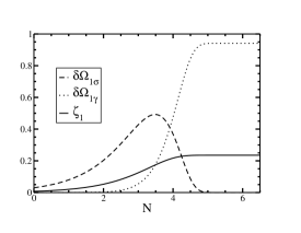
Figure 2: Evolution of the total curvature perturbation, $\zeta_{1}$, and the normalised density perturbations at first order as a function of the number of e-foldings, starting with $\zeta_{1\sigma}=1$ and initial density and decay rate $\Omega_{0\sigma}=10^{-2}$ and $\Gamma/H=10^{-3}$, corresponding to $p_{\rm{in}}=0.32$.

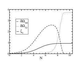
Figure 3: Same as Fig. 2 but with $\Gamma/H=10^{-6}$ initially, corresponding to $p_{\rm{in}}=10$.

The perturbed energy transfer rates are given from Eq. (34) at first order as

$$\delta Q_{1\sigma}=-\Gamma\delta\rho_{1\sigma}\,,\qquad\delta Q_{1\gamma}=\Gamma\delta\rho_{1\sigma}\,.$$ (42)

The evolution equations at first order are from Eq. (15) and Eqs. (33), and using (42) in terms of the normalised energy densities defined in Eq. (22) given by

$$\delta\Omega_{1\sigma}^{\prime}+\left[\frac{3-2g}{1-g}-\frac{\Omega_{0\sigma}}{2}\frac{6-5g}{1-g}-4\Omega_{0\gamma}\right]\delta\Omega_{1\sigma}-\frac{\Omega_{0\sigma}}{2}\frac{g}{1-g}\delta\Omega_{1\gamma}=0\,,$$ (43)

$$\delta\Omega_{1\gamma}^{\prime}+\left[4\left(1-\Omega_{0\gamma}\right)-\frac{6-7g}{1-g}\frac{\Omega_{0\sigma}}{2}\right]\delta\Omega_{1\gamma}-\frac{g}{1-g}\left(1-\frac{\Omega_{0\sigma}}{2}\right)\delta\Omega_{1\sigma}=0\,.$$ (44)

The curvature perturbations at first order on uniform curvaton and radiation density hypersurfaces are from Eq. (19) given by

$$\zeta_{1\sigma} = \frac{1-g}{(3-2g)\Omega_{0\sigma}}\delta\Omega_{1\sigma}\,,$$ (45)

$$\zeta_{1\gamma} = \frac{1-g}{4\left(1-g\right)\Omega_{0\gamma}-g\Omega_{0\sigma}}\delta\Omega_{1\gamma}\,.$$ (46)

The curvature perturbation on uniform total density slices in terms of the new variables is given by

$$\zeta_{1}=\frac{\delta\Omega_{1\sigma}+\delta\Omega_{1\gamma}}{3\Omega_{0\sigma}+4\Omega_{0\gamma}}\,.$$ (47)

Solutions for the equation system (43) and (44) are given in Figs. 2 and 3 for two different sets of initial conditions, $\Omega_{0\sigma}=10^{-2}$ and $\Gamma/H=10^{-3}$ and $\Omega_{0\sigma}=10^{-2}$ and $\Gamma/H=10^{-6}$, corresponding to $p_{\rm{in}}=0.32$ and $p_{\rm{in}}=10$, respectively. Using Eq. (47) we also plot the evolution of $\zeta_{1}$. For the perturbations we use the initial conditions

$$\zeta_{1\sigma,\rm{in}}=1\,,\qquad\zeta_{1\gamma,\rm{in}}=0\,,$$ (48)

which can be easily translated in initial conditions for $\delta\Omega_{1\sigma}$ using Eq. (45), and facilitates comparison with Ref. MWU .

Note that the values for $\delta\Omega_{1\sigma}$ and $\delta\Omega_{1\gamma}$ can exceed $1$, as can be seen in Fig. 3. This doesn’t indicate the “breakdown of perturbation theory” or anything dramatic like it, but is merely an artifact of normalising the density perturbations by the total background density $\rho_{0}$, which can itself be small. As in the background, the normalised energy densities together with the choice of time coordinate give a particularly neat system of governing equations.

III.3 Second order

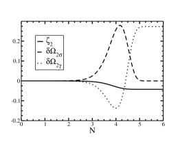
Figure 4: Evolution of the total curvature perturbation, $\zeta_{2}$, and the normalised density perturbations at second order as a function of the number of e-foldings, with initially $\zeta_{1\sigma,\rm{in}}=1$ and density and decay rate $\Omega_{0\sigma}=10^{-2}$ and $\Gamma/H=10^{-3}$, corresponding to $p_{\rm{in}}=0.32$.

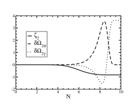
Figure 5: Same as Fig. 4 but with $\Gamma/H=10^{-6}$ initially, corresponding to $p_{\rm{in}}=10$.

The perturbed energy transfer rates are given from Eq. (34) at second order as

$$\delta Q_{2\sigma}=-\Gamma\delta\rho_{2\sigma}\,,\qquad\delta Q_{2\gamma}=\Gamma\delta\rho_{2\sigma}\,.$$ (49)

We then find evolution equations at second order from Eq. (24) and using Eqs. (33) and (49) in terms of the normalised energy densities defined above in Eqs. (22) and (31) to be

$$\delta\Omega_{2\sigma}^{\prime} + \left[\frac{3-2g}{1-g}-\frac{\Omega_{0\sigma}}{2}\frac{6-5g}{1-g}-4\Omega_{0\gamma}\right]\delta\Omega_{2\sigma}-\frac{\Omega_{0\sigma}}{2}\frac{g}{1-g}\delta\Omega_{2\gamma}$$ (50)

$$\qquad-\frac{g}{1-g}\left(\delta\Omega_{1\sigma}+\delta\Omega_{1\gamma}\right)\left[\delta\Omega_{1\sigma}-\frac{3}{4}\Omega_{0\sigma}\left(\delta\Omega_{1\sigma}+\delta\Omega_{1\gamma}\right)\right]=0\,,$$

$$\delta\Omega_{2\gamma}^{\prime} + \left[4\left(1-\Omega_{0\gamma}\right)-\frac{6-7g}{1-g}\frac{\Omega_{0\sigma}}{2}\right]\delta\Omega_{2\gamma}-\left(1-\frac{\Omega_{0\sigma}}{2}\right)\frac{g}{1-g}\delta\Omega_{2\sigma}$$ (51)

$$\qquad+\frac{g}{1-g}\left(\delta\Omega_{1\sigma}+\delta\Omega_{1\gamma}\right)\left[\delta\Omega_{1\sigma}-\frac{3}{4}\Omega_{0\sigma}\left(\delta\Omega_{1\sigma}+\delta\Omega_{1\gamma}\right)\right]=0\,.$$

The adiabatic sound speed in a multi-fluid system is given above in Eq. (30) and we find for the two-fluid curvaton model

$$c_{\rm{s}}^{2}=\frac{1}{3}\frac{4\left(1-g\right)\Omega_{0\gamma}-g\Omega_{0\sigma}}{\left(1-g\right)\left(3\Omega_{0\sigma}+4\Omega_{0\gamma}\right)}\,.$$ (52)

The curvature perturbation on uniform total density hypersurfaces at second order in terms of the normalised quantities is

$$\zeta_{2}=\frac{\delta\Omega_{2\sigma}+\delta\Omega_{2\gamma}}{3\Omega_{0\sigma}+4\Omega_{0\gamma}}-\left(1-3c_{\rm{s}}^{2}\right)\left(\frac{\delta\Omega_{1\sigma}+\delta\Omega_{1\gamma}}{3\Omega_{0\sigma}+4\Omega_{0\gamma}}\right)^{2}-2\frac{\left(\delta\Omega_{1\sigma}+\delta\Omega_{1\gamma}\right)\delta\Omega_{1\gamma}}{\left(3\Omega_{0\sigma}+4\Omega_{0\gamma}\right)^{2}}\,,$$ (53)

where $c_{\rm{s}}^{2}$ is given above in Eq. (52).

The system of equations (50) and (51) is readily integrated using a standard fourth order Runge-Kutta solver NR . We give the solutions for this system of equations for the two different sets of initial conditions, $\Omega_{0\sigma}=10^{-2}$ and $\Gamma/H=10^{-3}$ and $\Omega_{0\sigma}=10^{-2}$ and $\Gamma/H=10^{-6}$, corresponding to $p_{\rm{in}}=0.32$ and $p_{\rm{in}}=10$, in Figs. 4 and 5. Using Eq. (53) we also plot the evolution of $\zeta_{2}$. The initial conditions for the second order perturbations are chosen as

$$\delta\Omega_{2\sigma,\rm{in}}=0\,,\qquad\delta\Omega_{2\gamma,\rm{in}}=0\,.$$ (54)

Note that the values for $\delta\Omega_{2\sigma}$ and $\delta\Omega_{2\gamma}$ can exceed $1$, as can be seen in Fig. 5. As at first order, this is merely an artifact of using normalised energy densities. We do however see a new effect: at second order the energy densities $\delta\rho_{2\alpha}$ can and do become negative, as can be seen clearly in Figs. 4 and 5. This is a “real” effect and not a normalisation artifact since $\rho_{0}\geq 0$ always. However, the total energy density $\rho$ as given by summing over all the terms in the power series expansion Eq. (6), again stays positive definite.

IV Relating the perturbative treatment to the $\Delta N$ formalism

The $\Delta N$ formalism SaSt95 provides a simple tool to calculate the curvature perturbation on large scales at all orders in the perturbations on scales larger than the horizon SaTa ; LMS ; Lyth:2005fi . The main simplification compared to cosmological perturbation theory stems from the fact that we only need the background evolution equations, and not the full governing equations at all orders of interest. However, if there is no analytic solution the numerics necessary to get a result turn out to be quite involved as can be seen below. Nevertheless, we shall outline the calculation in the following.

The $\Delta N$ formalism relates the curvature perturbation on uniform density hypersurfaces to the perturbation in the number of e-foldings from the uniform density to the flat slicing,

$$\zeta=\delta N\,.$$ (55)

To get the number of e-foldings $N$ we use Eq. (40) to get $dN$ in terms of $dg$, and integrate,

$$N=2\int^{g_{\rm{fin}}}_{g_{\rm{in}}}\frac{dg}{g\left(1-g\right)\left(4-\Omega_{0\sigma}\right)}\,.$$ (56)

The curvature perturbation in the $\Delta N$ formalism is then given from Eq. (55) by expanding $N$ in a Taylor series, which leads in the curvaton case to Lyth:2005fi ; Lyth2006

$$\zeta=\frac{\partial N}{\partial\Omega_{0\sigma\rm{in}}}\delta\Omega_{\sigma\rm{in}}+\frac{1}{2}\frac{\partial^{2}N}{\partial\Omega_{0\sigma\rm{in}}^{2}}\delta\Omega_{\sigma\rm{in}}^{2}\,,$$ (57)

where the partial differentials are

$$\frac{\partial N}{\partial\Omega_{0\sigma\rm{in}}} = 2\int^{g}_{g_{1}}\frac{dg}{g\left(1-g\right)\left(4-\Omega_{0\sigma}\right)^{2}}\frac{\partial\Omega_{0\sigma}}{\partial\Omega_{0\sigma\rm{in}}}\,,$$ (58)

$$\frac{\partial^{2}N}{\partial\Omega_{0\sigma\rm{in}}^{2}} = 2\int^{g}_{g_{\rm{in}}}\frac{dg}{g\left(1-g\right)\left(4-\Omega_{0\sigma}\right)^{2}}\left[\frac{\partial^{2}\Omega_{0\sigma}}{\partial\Omega_{0\sigma\rm{in}}^{2}}+\frac{2}{\left(4-\Omega_{0\sigma}\right)}\left(\frac{\partial\Omega_{0\sigma}}{\partial\Omega_{0\sigma\rm{in}}}\right)^{2}\right]\,.$$ (59)

Note, that to make contact with first and second order perturbation theory, $\zeta$ and $\delta\Omega_{\sigma\rm{in}}$ have to be expanded up to second order, where in this case the second order curvature perturbation corresponds to $\zeta_{2\rm{SB}}$, defined above in Eq. (32), related to $\zeta_{2}$ as specified in Eq. (29).

Although in principle we can evaluate the integrals in Eqs. (58) and (59) numerically and then differentiate them with respect to the initial conditions to get the value of $\zeta$, this is (arguably) more difficult than solving a set of coupled differential equations. We therefore don’t use the $\Delta N$ formalism in the following sections, and solve instead the system of differential equations presented in Section III.

However, the $\Delta N$ formalism is used in Ref. misao_jussi_david in another numerical study of the curvaton scenario. The results are similar to the ones presented in this paper, but the computing time required in the $\Delta N$ case is increased by factor of roughly $\sim 100$ compared to solving the system of differential equations presented in Section III.

V The non-linearity parameter $f_{\rm{NL}}$: results and discussion

In this section we give the non-linearity parameter $f_{\rm{NL}}$ calculated numerically using the governing equations at second order of Sections II and III and compare it to previous numerical first order results and analytical sudden decay estimates.

The non-gaussianity parameter $f_{\rm{NL}}$ is defined as Komatsu2001 ; Lyth:2005fi

$$\zeta={\zeta_{\rm{g}}}+\frac{3}{5}f_{\rm{NL}}\left({\zeta_{\rm{g}}}^{2}-{\bar{{\zeta_{\rm{g}}}}}^{2}\right)\,,$$ (60)

where $\zeta$ is the curvature perturbation at all orders, ${\zeta_{\rm{g}}}$ the gaussian part of $\zeta$, and the “bar” denotes the spatial average. There has been some confusion in the literature as to the sign of $f_{\rm{NL}}$, which becomes relevant if the result is compared with observations. The sign convention chosen here coincides with the one used originally by Komatsu and Spergel Komatsu2001 and adopted by most observational studies, and corrects the sign error introduced in Ref. LUW and carried through in much subsequent work Bartolo2003 ; Bartolo:2004if .

We now relate the curvaton field fluctuations to the curvaton fluid energy density. The energy density in the curvaton field can be approximated by

$$\rho_{\sigma}=\frac{1}{2}m^{2}\sigma^{2}\,,$$ (61)

where $m$ is the curvaton mass and $\sigma$ is the amplitude of the curvaton field. Expanding the curvaton amplitude to first order, $\sigma=\sigma_{0}+\delta\sigma_{1}$, we get from Eq. (61),

$$\rho_{0\sigma}=\frac{1}{2}m^{2}\sigma_{0}^{2}\,,$$ (62)

$$\frac{\delta\rho_{1\sigma}}{\rho_{0\sigma}}\equiv 2\frac{\delta\sigma_{1}}{\sigma_{0}}+\left(\frac{\delta\sigma_{1}}{\sigma_{0}}\right)^{2}\,,$$ (63)

$$\frac{\delta\rho_{2\sigma}}{\rho_{0\sigma}}\equiv 0\,.$$ (64)

Note, that including the quadratic term $(\delta\sigma_{1}/\sigma_{0})^{2}$ in the first order energy density and setting the second order energy density perturbation to zero is just convention, following Ref. LUW . In Ref. Bartolo2003 this term is included in the second order energy density perturbation of the curvaton fluid. This choice doesn’t effect the final results.

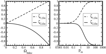
Figure 6: The final values of the normalised curvature perturbations at first and second order, $\zeta_{1,\rm{in}}$ and $\zeta_{2,\rm{in}}$, for an initial value $\zeta_{1\sigma,\rm{in}}=1$, versus the background curvaton energy density at decay, $\Omega_{\sigma\rm{dec}}$, in the left panel and versus $p_{\rm{in}}$ in the right panel.

V.1 Sudden decay

In the sudden decay one assumes that the curvaton doesn’t decay into radiation until a time $t_{\rm{dec}}$, when all of the curvaton energy density decays suddenly; the normalised energy density of the curvaton at decay is denoted $\Omega_{\sigma\rm{dec}}$. The sudden decay approximation has been widely used in the literature to study the curvaton scenario without having to resort to numerical calculations, see e.g. Refs.curvaton ; LUW ; Bartolo2003 ; Lyth:2005fi . In order to be able to compare the sudden decay approximation to the numerical calculation we now give a prescription to calculate $\Omega_{\sigma\rm{dec}}$.

The normalised background energy density can be approximated by Linde2005 ; Lyth2006 ; curvaton

$$\Omega_{0\sigma}=\frac{\sigma_{0}^{2}}{\sigma_{0}^{2}+6M_{\rm{pl}}^{2}\sqrt{\frac{H}{m}}}\,,$$ (65)

where $M_{\rm{pl}}^{2}=(8\pi G)^{-1}$. Assuming that the evolution of the background curvaton amplitude from the initial time up to curvaton decay is negligible and using that initially $H_{\rm{in}}=m$, and at curvaton decay $H_{\rm{dec}}=\Gamma$ we can use Eq. (65) to relate the parameter $p_{\rm{in}}$, defined in Eq. (41), to the background energy density of the curvaton at decay. We therefore define

$$\Omega_{\sigma\rm{dec}}\equiv\frac{p_{\rm{in}}}{1+p_{\rm{in}}}\,,$$ (66)

as energy density of the curvaton in the sudden decay approximation. The agreement $\Omega_{\sigma\rm{dec}}$ defined in Eq. (66) with $\Omega_{\sigma\rm{dec}}$ used in Ref. MWU is quite good, and we use the definition (66) in the following to compare our numerical results with the sudden decay approximation.

We now briefly review the results of previous analytical treatments using the sudden decay approximation to calculate the non-linearity parameter $f_{\rm{NL}}$ in the curvaton scenario.

The non-linearity parameter in the sudden decay approximation using first order perturbation theory, however using the definition of the first order energy density perturbation quadratic in the curvaton fluctuations Eq. (63), is curvaton ; LUW

$$f_{\rm{NL}}=\frac{5}{4\Omega_{\sigma\rm{dec}}}\,.$$ (67)

Using second order perturbation theory the non-linearity parameter in the sudden decay approximation was found to be Bartolo2003 ; Lyth:2005du

$$f_{\rm{NL}}=\frac{5}{4\Omega_{\sigma\rm{dec}}}-\frac{5}{6}\Omega_{\sigma\rm{dec}}-\frac{5}{3}\,.$$ (68)

V.2 Numerical solutions

The transfer parameter at first order relating the initial curvature perturbation on uniform curvaton density hypersurfaces to the final value of the total curvature perturbation is defined as curvaton ; LUW ; MWU

$$r_{1}\equiv\frac{\zeta_{1,\rm{fin}}}{\zeta_{1\sigma,\rm{in}}}\,.$$ (69)

We define the transfer parameter at second order

$$r_{2}\equiv\frac{\zeta_{2,\rm{fin}}}{\zeta_{1\sigma,\rm{in}}^{2}}\,,$$ (70)

relating the final value of the total curvature perturbation to the initial curvature perturbation on uniform curvaton slices. The values for $r_{1}$ and $r_{2}$ coincide for our choice of initial condition, $\zeta_{1\sigma,\rm{in}}=1$, with the final values of the curvature perturbations at first and second order, $\zeta_{1,\rm{fin}}$ and $\zeta_{2,\rm{fin}}$, and are given in Fig. 6 versus $\Omega_{\sigma\rm{dec}}$ and $p_{\rm{in}}$.

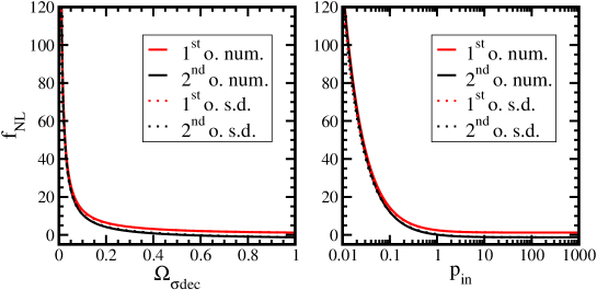
Figure 7: The nonlinearity parameter $f_{\rm{NL}}$ versus $\Omega_{\sigma\rm{dec}}$ and $p_{\rm{in}}$: numerical results and sudden decay approximation at first and second order.

The non-linearity parameter using first order perturbation theory is given in terms of the transfer parameter defined in Eq. (69) as LUW ; MWU

$$f_{\rm{NL}}=\frac{5}{4r_{1}}\,.$$ (71)

Using second order perturbation theory we find the non-linearity parameter $f_{\rm{NL}}$ from Eq. (60), expanding $\zeta$ to second order, and get in terms of the transfer parameters at first and second order

$$f_{\rm{NL}}=\frac{5}{4r_{1}}+\frac{5}{6}\frac{r_{2}}{{r_{1}}^{2}}-\frac{5}{3}\,.$$ (72)

In the above calculations we identified ${\zeta_{\rm{g}}}$ with the part of $\zeta_{1}$ linear in the curvaton field fluctuation, i.e. the first term in Eq. (63).

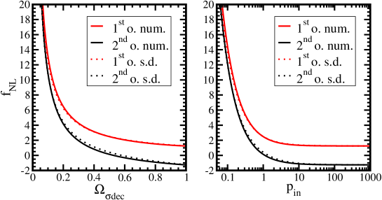
Figure 8: The nonlinearity parameter $f_{\rm{NL}}$ versus $\Omega_{\sigma\rm{dec}}$ and $p_{\rm{in}}$: numerical results and sudden decay approximation at first and second order, detail of Fig. 7.

We can finally relate the transfer parameters $r_{1}$ and $r_{2}$ to the total curvature perturbation, $\zeta=\zeta_{1}+\frac{1}{2}\zeta_{2}$, evaluated after the curvaton has decayed,

$$\zeta_{\rm{fin}}=r_{1}\zeta_{1\sigma,\rm{in}}+\frac{1}{2}r_{2}\zeta_{1\sigma,\rm{in}}^{2}\,.$$ (73)

Using the definition of the curvature perturbation on uniform curvaton density hypersurfaces, Eq. (19), and the expression for the curvaton energy density in terms of the curvaton amplitude, Eq. (63), we get

$$\zeta=\frac{2}{3}r_{1}\frac{\delta\sigma_{1}}{\sigma_{0}}+\frac{1}{3}\left(r_{1}+\frac{2}{3}r_{2}\right)\left(\frac{\delta\sigma_{1}}{\sigma_{0}}\right)^{2}\,.$$ (74)

We can compare these results to the expression found using the $\Delta N$-formalism, expressed in terms of the curvaton perturbation (instead of the normalised energy perturbation used in Section IV) Lyth:2005fi ; Lyth2006 ,

$$\zeta_{\rm{SB}}=N_{,\sigma}\delta\sigma+\frac{1}{2}N_{,\sigma\sigma}\delta\sigma^{2}\,.$$ (75)

The curvature perturbation employed in the $\Delta N$-formalism, $\zeta_{2\rm{SB}}$, is related to $\zeta$ by Eq. (32), and we get

$$\zeta_{\rm{SB}}=\frac{2}{3}r_{1}\frac{\delta\sigma_{1}}{\sigma_{0}}+\frac{1}{3}\left(r_{1}+\frac{2}{3}r_{2}-\frac{4}{3}r_{1}^{2}\right)\left(\frac{\delta\sigma_{1}}{\sigma_{0}}\right)^{2}\,,$$ (76)

and therefore

$$N_{,\sigma}=\frac{2}{3}\frac{r_{1}}{\sigma_{0}}\,,\qquad N_{,\sigma\sigma}=\frac{2}{3\sigma_{0}^{2}}\left(r_{1}+\frac{2}{3}r_{2}-\frac{4}{3}r_{1}^{2}\right)\,.$$ (77)

V.3 Curvaton amplitude evolution

So far we assumed that the curvaton field doesn’t evolve between the end of inflation and curvaton decay. In order to allow for the evolution of curvaton field amplitude $\sigma$ we assume that it depends on the initial value set during inflation $\sigma_{\rm{e}}$ by $\sigma=\sigma(\sigma_{\rm{e}})$ which gives for the curvaton field fluctuation Lyth:2003dt ; Enqvist:2005pg ; Lyth2006

$$\delta\sigma=\sigma^{\prime}\delta\sigma_{\rm{e}}+\frac{1}{2}\sigma^{\prime\prime}\delta\sigma_{\rm{e}}^{2}\,,$$ (78)

where $\sigma^{\prime}\equiv\partial\sigma/\partial\sigma_{\rm{e}}$. For the first order energy density we then find (including again the quadratic term)

$$\frac{\delta\rho_{1\sigma}}{\rho_{0\sigma}}=2\frac{\delta\sigma_{\rm{e}1}}{\sigma_{0}}\sigma_{0}^{\prime}+\left(\frac{\delta\sigma_{\rm{e}1}}{\sigma_{0}}\right)^{2}\left(1+\sigma_{0}\frac{\sigma_{0}^{\prime\prime}}{{{\sigma_{0}^{\prime}}^{2}}}\right){\sigma_{0}^{\prime}}^{2}\,.$$ (79)

We therefore get for the non-linearity parameter

$$f_{\rm{NL}}=\left[\frac{5}{4r_{1}}+\frac{5}{6}\frac{r_{2}}{{r_{1}}^{2}}\right]\left(1+\sigma_{0}\frac{\sigma^{\prime\prime}_{0}}{{{\sigma^{\prime}_{0}}^{2}}}\right)-\frac{5}{3}\,,$$ (80)

instead of Eq. (72) above. However, in order to calculate a numerical value for $f_{\rm{NL}}$ we now have to calculate the evolution of $\sigma$ in detail and specify a curvaton model. We shall therefore not pursue this issue further and refer to Ref. Enqvist:2005pg where this issue was studied in detail.

V.4 Results and discussion

Our results are summed up in Figs. 7-9: in Figs. 7 and 8 we plot the non-linearity parameter calculated numerically using Eq. (71) at first order and Eq. (72) at second order for two different parametrisations, namely $\Omega_{\sigma\rm{dec}}$and $p_{\rm{in}}$. In the same figures we also plot the non-linearity parameter $f_{\rm{NL}}$ in the sudden decay approximation at first and second order from Eqs. (67) and (68), respectively. We truncated the graphs at $f_{\rm{NL}}=120$ in accordance with the current observational bounds (see below). We first note how well the sudden decay approximation and the numerical solution at first and second order agree. However, at first order we find that $f_{\rm{NL}}=5/4$ for $\Omega_{\sigma\rm{dec}}=1$ or large values of $p_{\rm{in}}$, whereas including the second order effects we get $f_{\rm{NL}}=-5/4$ for $\Omega_{\sigma\rm{dec}}=1$ or large values of $p_{\rm{in}}$.

In Fig. 9 we plot the difference between the non-linearity parameter obtained numerically and using the sudden decay approximation, both at second order,

$$\Delta f_{\rm{NL}}\equiv f_{\rm{NL}}\Big{|}_{\rm{numerical}}-f_{\rm{NL}}\Big{|}_{\rm{suddendecay}}\,.$$ (81)

We now see more clearly the excellent agreement of the sudden decay approximation for large parameters $p_{\rm{in}}$ and $\Omega_{\sigma\rm{dec}}$. However, for small $p_{\rm{in}}$ and $\Omega_{\sigma\rm{dec}}$ the sudden decay approximation works less well, deviating from the numerical solution by up to $10\%$.

Figure 9: The difference of the numerical and the sudden decay approximation value of the non-linearity parameter, $\Delta f_{\rm{NL}}$, versus $\Omega_{\sigma\rm{dec}}$ and $p_{\rm{in}}$.

We finally give the observational constraint on the non-linearity parameter $f_{\rm{NL}}$ from the recently published WMAP three-year data. Spergel et al. found Spergel : $-54<f_{\rm{NL}}<114$ (at $95\%$ confidence level). The curvaton model is therefore well within the current observational bounds. However, if future observations give a large negative value for the non-linearity parameter, the curvaton model would be ruled out, at least without strong evolution of the curvaton amplitude from the beginning of the oscillations to curvaton decay, as pointed in in Section V.3 above.

Appendix A Governing equations

Here we first give the governing equations on large scales in the general case without gauge restrictions and then the equations given in Section III in terms of non-normalised energy densities.

A.1 Governing equations without gauge restriction

In this subsection we give the governing equations on large scales in the general case without any gauge restrictions, i.e. without choosing a particular hypersurface.

A.1.1 First order

Energy conservation of the $\alpha$-fluid is given from Eq. (4) at first order as

$$\dot{{\delta\rho_{1\alpha}}}+3H\left({\delta\rho_{1\alpha}}+{\delta P_{1\alpha}}\right)-3\dot{\psi}_{1}\left(\rho_{0\alpha}+P_{0\alpha}\right)-Q_{0\alpha}\phi_{1}-{\delta Q_{1\alpha}}=0\,.$$ (82)

Total energy conservation follows from Eq. (82) above, and using Eqs. (5) and (16), is given by

$$\dot{{\delta\rho_{1}}}+3H\left({\delta\rho_{1}}+{\delta P_{1}}\right)-3\dot{\psi}_{1}\left(\rho_{0}+P_{0}\right)=0\,.$$ (83)

The $0-0$ Einstein equation is given from Eq. (1) as

$$3H\left(H\phi_{1}+\dot{\psi}_{1}\right)=-4\pi G\delta\rho_{1}\,.$$ (84)

A.1.2 Second order

Energy conservation of the $\alpha$-fluid is given from Eq. (4) at second order as

$$\dot{{\delta\rho_{2\alpha}}} + 3H\left({\delta\rho_{2\alpha}}+{\delta P_{2\alpha}}\right)-3\dot{\psi}_{2}\left(\rho_{0\alpha}+P_{0\alpha}\right)-6\left(\delta\rho_{1\alpha}+\delta P_{1\alpha}\right)\dot{\psi}_{1}-12\left(\rho_{0\alpha}+P_{0\alpha}\right)\dot{\psi}_{1}\psi_{1}$$ (85)

$$- Q_{0\alpha}\left(\phi_{2}-\phi_{1}^{2}\right)-2\phi_{1}{\delta Q_{1\alpha}}-{\delta Q_{2\alpha}}=0\,,$$

and, following a similar route as at first order, the conservation of the total energy density is given at second order by

$$\dot{{\delta\rho_{2}}} + 3H\left({\delta\rho_{2}}+{\delta P_{2}}\right)-3\dot{\psi}_{2}\left(\rho_{0}+P_{0}\right)-6\left(\delta\rho_{1}+\delta P_{1}\right)\dot{\psi}_{1}-12\left(\rho_{0}+P_{0}\right)\dot{\psi}_{1}\psi_{1}=0\,,$$ (86)

and the $0-0$ Einstein equation is given by

$$3H^{2}\left(\phi_{2}-4\phi_{1}^{2}\right)+3\left(H\dot{\psi}_{2}-{\dot{\psi}_{1}}^{2}\right)+12H\dot{\psi}_{1}\left(\psi_{1}-\phi_{1}\right)=-4\pi G\delta\rho_{2}\,.$$ (87)

A.2 Governing equations in terms of non-normalised energy densities

In this subsection we give the governing equations presented in Sections III.2 and III.3 above in terms of the normalised quantities in terms of the non-normalised energy densities and decay rate. We use the number of e-foldings $N$ as time coordinate and work throughout in the flat gauge (omitting the “tilde”).

We get at first order

$$\delta\rho_{1\sigma}^{\prime}+\left(3+\frac{\Gamma}{H}\right)\delta\rho_{1\sigma}-\frac{1}{2}\frac{\Gamma}{H}\frac{\rho_{0\sigma}}{\rho_{0}}\delta\rho_{1}=0\,,$$ (88)

$$\delta\rho_{1\gamma}^{\prime}+4\delta\rho_{1\gamma}-\frac{\Gamma}{H}\delta\rho_{1\sigma}+\frac{1}{2}\frac{\Gamma}{H}\frac{\rho_{0\sigma}}{\rho_{0}}\delta\rho_{1}=0\,,$$ (89)

and at second order

$$\delta\rho_{2\sigma}^{\prime}+\left(3+\frac{\Gamma}{H}\right)\delta\rho_{2\sigma}-\frac{\Gamma}{H}\frac{\delta\rho_{1}}{\rho_{0}}\delta\rho_{1\sigma}+\frac{\Gamma}{H}\frac{\rho_{0\sigma}}{\rho_{0}}\left(\frac{3}{4}\frac{{\delta\rho_{1}}^{2}}{\rho_{0}}-\frac{1}{2}\delta\rho_{2}\right)=0\,,$$ (90)

$$\delta\rho_{2\gamma}^{\prime}+4\delta\rho_{2\gamma}-\frac{\Gamma}{H}\delta\rho_{2\sigma}+\frac{\Gamma}{H}\frac{\delta\rho_{1}}{\rho_{0}}\delta\rho_{1\sigma}-\frac{\Gamma}{H}\frac{\rho_{0\sigma}}{\rho_{0}}\left(\frac{3}{4}\frac{{\delta\rho_{1}}^{2}}{\rho_{0}}-\frac{1}{2}\delta\rho_{2}\right)=0\,.$$ (91)

References

(1)http://lambda.gsfc.nasa.gov/
(2)
A. R. Liddle and D. H. Lyth,
Cosmological inflation and large-scale structure, CUP,
Cambridge, UK (2000).
(3)
D. H. Lyth and D. Wands,
Phys. Lett. B 524, 5 (2002)
[arXiv:hep-ph/0110002].
(4)
K. Enqvist and M. S. Sloth,
Nucl. Phys. B 626, 395 (2002) [arXiv:hep-ph/0109214].
(5)
T. Moroi and T. Takahashi,
Phys. Lett. B 522, 215 (2001) [Erratum-ibid. B 539,
303 (2002)] [arXiv:hep-ph/0110096];
Phys. Rev. D 66, 063501 (2002)
[arXiv:hep-ph/0206026].
(6)
D. H. Lyth, C. Ungarelli and D. Wands,
Phys. Rev. D 67, 023503 (2003)
[arXiv:astro-ph/0208055].
(7)
K. A. Malik, D. Wands and C. Ungarelli,
Phys. Rev. D 67, 063516 (2003)
[arXiv:astro-ph/0211602].
(8)
D. H. Lyth,
Phys. Lett. B 579, 239 (2004)
[arXiv:hep-th/0308110].
(9)
S. Gupta, K. A. Malik and D. Wands,
Phys. Rev. D 69, 063513 (2004)
[arXiv:astro-ph/0311562].
(10)
K. Enqvist and S. Nurmi,
JCAP 0510, 013 (2005)
[arXiv:astro-ph/0508573].
(11)
A. Linde and V. Mukhanov,
arXiv:astro-ph/0511736.
(12)
D. H. Lyth,
JCAP 0606, 015 (2006)
[arXiv:astro-ph/0602285].
(13)
V. F. Mukhanov, L. R. W. Abramo and R. H. Brandenberger,
Phys. Rev. Lett. 78, 1624 (1997)
[arXiv:gr-qc/9609026].
(14)
M. Bruni, S. Matarrese, S. Mollerach and S. Sonego,
Class. Quant. Grav. 14, 2585 (1997)
[arXiv:gr-qc/9609040].
(15)
J. Maldacena,
JHEP 0305, 013 (2003)
[arXiv:astro-ph/0210603].
(16)
V. Acquaviva, N. Bartolo, S. Matarrese and A. Riotto,
Nucl. Phys. B 667, 119 (2003)
[arXiv:astro-ph/0209156].
(17)
K. Nakamura,
Prog. Theor. Phys. 110, 723 (2003)
[arXiv:gr-qc/0303090].
(18)
H. Noh and J. c. Hwang,
Phys. Rev. D 69, 104011 (2004).
(19)
N. Bartolo, S. Matarrese and A. Riotto,
Phys. Rev. D 65, 103505 (2002)
[arXiv:hep-ph/0112261].
(20)
N. Bartolo, S. Matarrese and A. Riotto,
Phys. Rev. D 69, 043503 (2004)
[arXiv:hep-ph/0309033].
(21)
F. Bernardeau and J. P. Uzan,
Phys. Rev. D 67, 121301 (2003)
[arXiv:astro-ph/0209330].
(22)
F. Bernardeau and J. P. Uzan,
Phys. Rev. D 66, 103506 (2002)
[arXiv:hep-ph/0207295].
(23)
K. A. Malik and D. Wands,
Class. Quant. Grav. 21, L65 (2004)
[arXiv:astro-ph/0307055].
(24)
N. Bartolo, E. Komatsu, S. Matarrese and A. Riotto,
Phys. Rept. 402, 103 (2004)
[arXiv:astro-ph/0406398].
(25)
N. Bartolo, S. Matarrese and A. Riotto,
Phys. Rev. Lett. 93, 231301 (2004)
[arXiv:astro-ph/0407505].
(26)
K. Enqvist and A. Vaihkonen,
JCAP 0409, 006 (2004)
[arXiv:hep-ph/0405103].
(27)
K. Tomita,
Phys. Rev. D 71, 083504 (2005)
[arXiv:astro-ph/0501663].
(28)
D. H. Lyth and Y. Rodriguez,
Phys. Rev. D 71, 123508 (2005)
[arXiv:astro-ph/0502578].
(29)
D. Seery and J. E. Lidsey,
JCAP 0509, 011 (2005)
[arXiv:astro-ph/0506056].
(30)
G. I. Rigopoulos and E. P. S. Shellard,
JCAP 0510, 006 (2005)
[arXiv:astro-ph/0405185].
(31)
G. I. Rigopoulos, E. P. S. Shellard and B. W. van Tent,
Phys. Rev. D 72, 083507 (2005)
[arXiv:astro-ph/0410486].
(32)
N. Bartolo, S. Matarrese and A. Riotto,
JCAP 0401, 003 (2004)
[arXiv:astro-ph/0309692].
(33)
K. A. Malik,
JCAP 0511, 005 (2005)
[arXiv:astro-ph/0506532].
(34) D. S. Salopek and J. R. Bond,
Phys. Rev. D 42 (1990) 3936.
(35)
M. Sasaki and E. D. Stewart,
Prog. Theor. Phys. 95, 71 (1996)
[arXiv:astro-ph/9507001].
(36)
M. Sasaki and T. Tanaka,
Prog. Theor. Phys. 99, 763 (1998)
[arXiv:gr-qc/9801017].
(37)
D. H. Lyth, K. A. Malik and M. Sasaki,
JCAP 0505, 004 (2005)
[arXiv:astro-ph/0411220].
(38)
D. H. Lyth and Y. Rodriguez,
Phys. Rev. Lett. 95, 121302 (2005)
[arXiv:astro-ph/0504045].
(39)
D. Langlois and F. Vernizzi,
Phys. Rev. D 72, 103501 (2005)
[arXiv:astro-ph/0509078].
(40)
K. A. Malik and D. Wands,
JCAP 0502, 007 (2005)
[arXiv:astro-ph/0411703].
(41)
H. Kodama and M. Sasaki,
Prog. Theor. Phys. Suppl. 78, 1 (1984).
(42)
D. Wands, K. A. Malik, D. H. Lyth and A. R. Liddle,
Phys. Rev. D 62, 043527 (2000)
[arXiv:astro-ph/0003278].
(43)
D. H. Lyth and D. Wands,
Phys. Rev. D 68, 103515 (2003)
[arXiv:astro-ph/0306498].
(44)
W. H. Press, S. A. Teukolsky, W. T. Vetterling, and B. P. Flannery
Numerical recipes in FORTRAN, Cambridge University Press (1992).
(45)
M. Sasaki, J. Valiviita, and D. Wands,
arXiv:astro-ph/0607627.
(46)
E. Komatsu and D. N. Spergel,
Phys. Rev. D 63, 063002 (2001)
[arXiv:astro-ph/0005036].
(47)
D. N. Spergel et al.,
arXiv:astro-ph/0603449.