A population of high-redshift type-2 quasars-I. Selection Criteria and Optical Spectra

Abstract

We discuss the relative merits of mid-infrared and X-ray selection of type-2 quasars. We describe the mid-infrared, near-infrared and radio selection criteria used to find a population of redshift $z\sim 2$ type-2 quasars which we previously argued suggests that most supermassive black hole growth in the Universe is obscured (Martínez-Sansigre et al., 2005). We present the optical spectra obtained from the William Herschel Telescope, and we compare the narrow emission line luminosity, radio luminosity and maximum size of jets to those of objects from radio-selected samples. This analysis suggests that these are genuine radio-quiet type-2 quasars, albeit the radio-bright end of this population. We also discuss the possibility of two different types of quasar obscuration, which could explain how the $\sim$2-3:1 ratio of type-2 to type-1 quasars preferred by modelling our population can be reconciled with the $\sim$1:1 ratio predicted by unified schemes.

1 Introduction

For a long time, a population of obscured (type-2) radio-quiet quasars has been postulated from modelling the hard (energies $\geq$ 1 keV) X-ray background as the sum of the emission from extragalactic sources. Comastri et al. (1995) assumed a population of absorbed active galactic nuclei (AGN: in this paper we use the term to encompass both Seyferts and quasars), with the same intrinsic spectrum and evolution as unobscured AGN, but with a range of obscuring Hydrogen column densities, $N_{\rm H}$, between $10^{25}$ and $10^{29}$ m^-2. The resulting best-fit ratio for absorbed ($N_{\rm H}>10^{26.5}$ m^-2) to unabsorbed ($N_{\rm H}<10^{26.5}$ m^-2) AGN was found to be $\sim$3:1. The model assumed the same distribution of obscuring column densities and redshifts for the low-X-ray luminosity objects ($L_{\rm X}<10^{37}$ W; the Seyferts) and the high-X-ray luminosity objects ($L_{\rm X}>10^{37}$ W; the quasars), including a population of highly obscured AGN (the Seyfert-2s and type-2 quasars).

According to unified schemes (Antonucci, 1993), type-2 quasars would consist of quasars with the symmetry axes perpendicular to the observer’s line of sight, so that the dusty torus around the accretion disk would be viewed edge on, obscuring the optically-bright accretion disk. The gas present in this torus will obscure the X rays via photoelectric absorption and Compton scattering. This unfavourable orientation means type-2 quasars do not outshine their host galaxy at (rest-frame) ultra-violet or optical wavelengths, as is the case with the unobscured (type-1) quasars. Type-2 quasars are therefore indistinguishable from normal galaxies in optical imaging surveys. If the torus has a half-opening angle of $\sim$ 40^∘, as appears to be the case in radio-loud samples (e.g. Willott et al., 2000), the population of type-2s is expected to be comparable in size to the type-1 population and not to outnumber it by a factor of $\sim$3.

A modification to the standard unified scheme is the “receding torus” model (Lawrence, 1991) in which the more luminous AGN sublimate the dust in the inner edge of the torus out to larger distances than the less luminous AGN. This leads to a larger opening angle for more luminous AGN, so the fraction of type-1 quasars increases as a function of bolometric luminosity. Such luminosity dependence of the type-2 to type-1 ratio is indeed found, for example, in radio-selected samples by Willott et al. (2000), in X-ray-selected samples by Ueda et al. (2003), and in spectroscopically selected samples by Simpson (2005).

More recent modelling of the hard X-ray background has consistently shown signs of a large population of obscured AGN (Wilman & Fabian, 1999; Worsley et al., 2005) and synthesis models have generally required a type-2 to type-1 ratio $\sim 3-4$:1 (Gilli et al., 2001; Ueda et al., 2003; Treister & Urry, 2005). However, the bulk of the sources required to fit the unresolved X-ray background have moderate redshifts ($z=0.5-1$) and X-ray luminosities ($L_{\rm X}\sim 10^{36}$ W) characteristic of Seyferts rather than quasars. The latest studies of the hard X-ray background indeed suggest a luminosity-dependent Compton-thin-type-2 to type-1 ratio, which decreases to $\,\stackrel{{\scriptstyle\raisebox{-0.60275pt}{$\textstyle<$}}}{{\sim}}\,$1:1 at the higher luminosities corresponding to quasars (Ueda et al., 2003; Treister & Urry, 2005). The true type-2 to type-1 ratio will remain unknown until the Compton-thick population is unveiled.

Deep hard X-ray surveys have now revealed a large population of obscured AGN (e.g. Alexander et al., 2003), but again most of these sources have moderate X-ray luminosities ($L_{\rm X}<10^{37}$ W) and are better described as Seyfert-2s rather than type-2 quasars. Amongst objects with X-ray luminosities large enough to qualify as quasars, the ratio of type-2 to type-1 objects appears to be only $\sim$1:1 (e.g. Zheng et al., 2004), although redshift completeness at faint optical magnitudes (m${}_{\rm R}>23$, Vega) may still be an issue. Despite the great progress with the deep hard X-ray surveys, at high energies (above 6-8 keV) only $\sim 50\%$ of the X-ray background is accounted for by individual sources, suggesting a substantial population of Compton-thick AGN which contribute to the hard X-ray background but are missing from current flux-limited X-ray surveys (Worsley et al., 2005). Indeed, a good example is the type-2 quasar IRAS FSC 10214+4724: this object, found in an IRAS 60 $\mu$m survey (Rowan-Robinson et al., 1991), has recently been found to be Compton-thick (Alexander et al., 2005).

An alternative strategy for looking for type-2 objects is to look for the mid-infrared emission. IRAS FSC 10214 +4724, at $z\sim 2.3$, is a classic type-2 object (e.g Serjeant et al., 1998). However, due to the limited sensitivity of IRAS, this object was only detected due to a huge gravitational lens magnification ($\sim$ 50) of the flux (Broadhurst & Lehar, 1995). The dramatic increase of mid-infrared sensitivity allowed by the Spitzer Space Telescope (Werner et al., 2004) means that similar objects can now be found without the ‘benefit’ of gravitational lensing, and mid-infrared selection should be sensitive to the Compton-thick quasars missed by X-rays.

Following the success of mid-infrared selection in finding type-2 radio-quiet quasars at $z\sim 0.5$ (Lacy et al., 2004, 2005a), we combined data from the Spitzer MIPS instrument at 24 $\mu$m (Marleau et al., 2004; Fadda et al., 2006), IRAC at 3.6 $\mu$m (Lacy et al., 2005) and from the Very Large Array (VLA) at 1.4 GHz (Condon et al., 2003) and devised strict selection criteria to hunt for higher redshift type-2s (Martínez-Sansigre et al., 2005). The trade-off between our method and X-ray selection, is that our quasars are intrinsically more luminous than AGN found in the deep hard X-ray surveys.

The format of this paper is as follows. In Section 2 we compare X-ray and mid-infrared selection of obscured quasars. In Section 3 we explain in detail the selection criteria which we used to find our sample of type-2 quasars. Section 4 deals with the observations while Section 5 describes the optical spectra and Section 6 compares the spectroscopic and photometric redshifts. In Section 7 we make the first composite radio-quiet type-2 spectrum. Section 8 is dedicated to comparing our sample to the well studied radio-loud samples. Finally, Section 9 summarises and discusses the implications of this population of type-2 quasars. Throughout this paper we adopt a $\Lambda$CDM cosmology with the following parameters: $h=H_{0}/(100~{}\rm km~{}s^{-1}~{}Mpc^{-1})=0.7$; $\Omega_{\rm m}=0.3$; $\Omega_{\Lambda}=0.7$.

2 Comparison between X-ray and Mid-infrared Selection

In the unified scheme for AGN (Antonucci, 1993), the central engine is surrounded by a torus of dust which will obscure the broad-line region from certain lines-of-sight. The optical classification for quasars is that type-1s should show broad lines (and strong optical-UV continuum) while the type-2s are those objects where the dusty torus is obscuring the broad line region, so only narrow lines are seen. This classification is concerned with the optical/UV properties, and Simpson et al. (1999) found that the dividing extinction for radio-selected (3CR and 3CRR) objects corresponded to $A_{\rm V}\raisebox{-2.58334pt}{$\,\stackrel{{\scriptstyle\raisebox{-0.60275pt}{$\textstyle>$}}}{{\sim}}\,$}5$, with a low fraction of objects with $A_{\rm V}$ in the range 5-15 and a large fraction with $A_{\rm V}\raisebox{-2.58334pt}{$\,\stackrel{{\scriptstyle\raisebox{-0.60275pt}{$\textstyle>$}}}{{\sim}}\,$}15$. Note also that the Simpson et al. (1999) study found that most type-1s ($A_{\rm V}\raisebox{-2.58334pt}{$\,\stackrel{{\scriptstyle\raisebox{-0.60275pt}{$\textstyle<$}}}{{\sim}}\,$}5$) had $A_{\rm V}\sim 0$, with only a small fraction lightly reddened ($A_{\rm V}\sim 1-5$). Gas and dust are responsible for obscuring the X-rays emitted from the central engine, and the geometrical distribution of the gas is almost certainly different from that of the dust. It is possible to imagine lines-of-sight which “graze” the dusty torus, leading to small amounts of extinction in the optical, but which go through significant additional amounts of gas. Such a line-of-sight would lead to a quasar classified as “reddened” (not type-2) in the optical ($A_{\rm V}\simeq 1-5$) but as type-2 ($N_{\rm H}\raisebox{-2.58334pt}{$\,\stackrel{{\scriptstyle\raisebox{-0.60275pt}{$\textstyle>$}}}{{\sim}}\,$}10^{26}$ m^-2) in X-rays. The converse situation, where an optically obscured quasar is barely absorbed in X-rays, is harder to envisage: any line of sight that passes through significant amounts of dust will lead to significant absorption in the X-rays. It is therefore unlikely that optical type-2 quasars will have negligible X-ray absorption. However, in edge-on sources, the nuclear soft X-ray emission can plausibly be scattered from an optically thin material located above or below the plane of the torus, leading to an optically-obscured AGN with a soft X-ray spectrum. Finally, obscuring material in the host galaxy of the AGN can further complicate interpretation. Independently of the orientation of the torus, dust and gas in the host galaxy can cause extinction and absorption with a huge range in $A_{\rm V}$ and $N_{\rm H}$.

X-ray and optical definitions of obscured AGN are therefore slightly different and the range of gas-to-dust ratios found by comparing dust-reddening in the optical or near-infrared and X-ray absorption suggests they are not always matched (e.g. Willott et al., 2003a; Urrutia et al., 2005; Wilkes et al., 2005). We note that we have used a mid-infrared plus radio selection, but since the role of the radio criterion was to avoid non-AGN contaminants (see Section 3), in this Section we can proceed to consider our technique as basically mid-infrared selection. The effect of adding the radio flux density cuts is to constrain the type-2 quasars selected to those at the high end of the radio-to-optical correlation for radio-quiet quasars of Cirasuolo et al. (2003), as described in in Section 3 and in Martínez-Sansigre et al. (2005). It is of course plausible that radio luminosity correlates in some complicated way with joint mid-infrared, X-ray detectability but we ignore this possibility here.

This section aims to compare the “merits” of mid-infrared and X-ray selection by considering a model quasar (described in section 2.1) with varying amounts of dust extinction (section 2.2) and different gas-to-dust ratios (section 2.3 ). We also consider the effects of different types of dust (section 2.5) and the orientation dependence of 24-$\mu$m emission (section 2.6).

2.1 Model quasar

We choose this quasar to have $M_{\rm B}=-25.7$ since this corresponds to the break in the optical quasar luminosity function at $z=2$ (Croom et al., 2004), the redshift of interest in the analysis in Martínez-Sansigre et al. (2005). The model quasar is assumed to have an intrinsic unreddened type-1 spectral energy distribution (SED), which we take from Rowan-Robinson (1995). This model covers the range between the (rest-frame) far-infrared and 4 keV. We need to complement this with a spectral energy distribution or SED that goes into the hard X-rays, so we assume the Madau et al. (1994) spectrum with the form $L_{\nu}\propto\nu^{-0.9}\rm exp(-\nu/\nu_{c})$ with $\rm h\nu_{c}=360~{}$keV. This intrinsic unabsorbed type-1 spectrum is chosen as it was used by Wilman & Fabian (1999) for the models we use for absorbed X-ray spectra. This is practically a flat X-ray SED, and in the range probed by observations at 24 $\mu$m (for $z\leq 5$), the SED is also flat ($L_{\nu}\propto\nu^{-1}$ so $\nu L_{\nu}\propto\nu^{0}$). We choose the normalisation to match the Rowan-Robinson (1995) SED at 2 keV.

2.2 Obscuration by dust

Starting with this type-1 SED, we proceed to model the obscuration of it with dust and gas. In recent times, the type of dust present in type-1 quasars (from the SDSS sample of Richards et al., 2002) has been described as “grey” and alternatively as similar to that of the Small Magellanic Clouds (SMC). Grey dust shows a relatively flat extinction law in the optical and UV, while SMC-type dust is characterised by a steep increase in the extinction at UV wavelengths. Milky Way (MW)-type dust has a UV extinction law which sits in between that of grey and SMC. Richards et al. (2003) and Hopkins et al. (2004) have found the dust in the SDSS type-1 sample to be closest to that found in the SMC, while Czerny et al. (2004) and Gaskell et al. (2004) argued that extinction curves flatten in the UV (grey dust). However, Willott (2005) has shown this implication of grey dust to be a selection effect. The main selection effect arises from measuring dust-reddening from a composite constructed from a flux limited sample: the UV part of the composite is constructed from the higher redshift quasars, which will only make the sample if they are intrinsically brighter and have very little extinction due to dust. This leads to a negative correlation between $E(B-V)$ and redshift, so that different parts of the composite spectrum are dominated by quasars with different amounts of dust. The result is a derived dust extinction curve which appears to flatten in the UV (see Willott, 2005, for more details).

We use the extinction curves from Pei (1992), with the extinction at (observed) 24 $\mu$m given in terms of the extinction at rest-frame visual band, $A_{\rm V}$, and a particular dust type. The quasars in the SDSS sample are all type-1s, and the dust discussed in the above paragraph is not necessarily associated with the torus. The SMC has sub-solar metallicity, while the nuclear regions around quasars have solar or super-solar metallicities, with dust properties probably closer to the MW. The effects of different types of dust are secondary compared to the gas-to-dust ratio, yet important, so we assume MW-dust in Figure 1 and discuss the effect of large magellanic cloud (LMC) and SMC-type dust in Section 2.5 and in Figure 2. Dust extinction is small at rest-frame 24 $\mu$m, yet the extreme obscuring columns present in the torus and the large redshifts discussed here mean that dust obscuration is not necessarily negligible at observed 24 $\mu$m. In particular, the 9.7 $\mu$m silicate absorption feature can have a very important effect on observed 24-$\mu$m flux density at $z\sim 1.5$ (and this feature is significantly deeper for SMC-type dust than for MW-type dust, Figure 2).

Figure 1: Hard X-ray flux ($S_{2-10\rm keV}$) versus 24-$\mu$m flux density ($S_{24~{}\mu\rm m}$) as a function of redshift for the model quasar described in Section 2. The tracks have the redshifts labelled at the positions marked with black dots at $z=$ 0.5, 1, 2, 3 and 5, and they show the effect on the quasar of MW-type dust with two different gas-to-dust ratios: $N_{\rm H}=1.9\times 10^{25}$ m${}^{-2}\times A_{\rm V}$ (Milky-Way, top two lines) and $N_{\rm H}=5\times 10^{26}$ m${}^{-2}\times A_{\rm V}$ (bottom two lines). Two tracks are drawn for each gas-to-dust ratio, $A_{\rm V}=5$ and 50 for the MW gas-to-dust ratio and $A_{\rm V}=5$ and 30 for the higher gas-to-dust ratio. The legend shows the combination of $A_{\rm V}$ and $N_{\rm H}$ [in log${10}(N_{\rm H}/\rm m^{-2})$] for each track. For the larger $A_{\rm V}$, the 9.7 $\mu$m silicate absorption feature can be seen as a “meander”. The dashed straight lines mark the limits for deep surveys covering large areas ($\sim 4-5$ deg²), while the solid straight lines show the limits for the GOODS fields, ultra-deep surveys which cover $\sim$ 0.1 deg². As an example of the large area Spitzer surveys, we have taken the flux density limit for 24-$\mu$m from the FLS (flux limit from Martínez-Sansigre et al., 2005, catalogue from Fadda et al., 2006), while the X-ray flux is taken from the ASCA survey of Ueda et al. (1999). For the deeper GOODS surveys, the 24-$\mu$m flux density limit is as quoted by Treister et al. (2006) and the X-ray flux limit is from Alexander et al. (2003). We note that the latter is actually in the 2-8 keV band (not 2-10 keV quoted here) but this relatively small difference does not alter our argument. Finally, the dotted lines are for the SXDF limit, a deep survey which has $\sim$1 deg² of deep X-ray data with 24-$\mu$m data from SWIRE (Lonsdale et al., 2003, Ueda et al. in prep).

2.3 X-ray absorption

In contrast to dust extinction, which increases with redshift, X-ray absorption decreases at higher frequencies, meaning X-ray samples benefit from a “negative K-correction”. The X-ray spectra of heavily absorbed quasars can only be modelled correctly via Monte-Carlo simulations, so we use the models of Wilman & Fabian (1999). These assume the intrinsic unabsorbed type-1 spectrum metioned earlier, and assume an Fe abundance 5-times solar, which provides a better fit to the hard X-ray backround. The particular models which we use here ignore the reflection component of X-ray spectra, as it has little effect on our discussion, and have a 2% scattered component. The obscuring column of Hydrogen, responsible for both types of absorption, is given here as a function of $A_{\rm V}$ by assuming a gas-to-dust ratio.

The Milky Way is known to have a gast-to-dust ratio such that $N_{\rm H}=1.9\times 10^{25}$ m${}^{-2}\times A_{\rm V}$ (Bohlin et al., 1978, note this is per magnitude of extinction in V band), while the SMC has $N_{\rm H}=1.8\times 10^{26}$ m${}^{-2}\times A_{\rm V}$ (Bouchet et al., 1985). Many AGN have been found to have higher gas-to-dust ratios than the MW (Maiolino et al., 2001; Willott et al., 2004). We therefore choose two representative values for the gas-to-dust ratio. The MW value is sometimes used as a “standard” gas-to-dust ratio. To show the effects of higher gas-to-dust ratios, we note that, for example, NGC 3281 has a value of $N_{\rm H}=3.2\times 10^{26}$ m${}^{-2}\times A_{\rm V}$ (Simpson, 1998b), while Urrutia et al. (2005) study one object with $N_{\rm H}\sim 7.7\times 10^{26}$ m${}^{-2}\times A_{\rm V}$ (FTM1004+1229, assuming a factor $R=3.0$, the average between the SMC and MW factors, to convert between $E(B-V)$ and $A_{\rm V}$). We therefore choose $N_{\rm H}=5\times 10^{26}$ m${}^{-2}\times A_{\rm V}$ as a realistic higher value to illustrate the effect of different gas-to-dust ratios. This is not claiming we encompass the whole range in gas-to-dust ratios, but is chosen to illustrate how mid-infrared and X-ray selection are affected by variations in gas-to-dust ratio. The higher value of gas-to-dust ratio $N_{\rm H}=5\times 10^{26}$ m${}^{-2}\times A_{\rm V}$ is high enough for an $A_{\rm V}=20$ type-2 quasar to be Compton-thick.

2.4 Comparison

Figure 1 shows the X-ray flux in the 2-10 keV band ($S_{2-10\rm keV}$) versus the 24-$\mu$m flux density ($S_{24\mu\rm m}$) for type-2 quasars with a range in $A_{\rm V}$. MW-type dust is used to obscure the 24-$\mu$m emission, and two different gas-to-dust ratios are used. The top set of curves are for a MW gas-to-dust ratio ($N_{\rm H}=1.9\times 10^{25}$ m${}^{-2}\times A_{\rm V}$), while the bottom curves are for $N_{\rm H}=5\times 10^{26}$ m${}^{-2}\times A_{\rm V}$. For the higher value of $A_{\rm V}$, the 9.7 $\mu$m silicate absorption feature can be seen as a “meander”. The caption in Figure 1 details the survey limits used for comparative purposes.

The effect of dust at observed 24 $\mu$m is small in the range $5\raisebox{-2.58334pt}{$\,\stackrel{{\scriptstyle\raisebox{-0.60275pt}{$\textstyle<$}}}{{\sim}}\,$}A_{\rm V}\raisebox{-2.58334pt}{$\,\stackrel{{\scriptstyle\raisebox{-0.60275pt}{$\textstyle<$}}}{{\sim}}\,$}50$. However, it is important to note that at $A_{\rm V}\sim 50$, type-2s will start to drop out of 24-$\mu$m selection (for the larger area surveys) at $z\sim 1.5$ (due to the silicate absorption) and at $z\raisebox{-2.58334pt}{$\,\stackrel{{\scriptstyle\raisebox{-0.60275pt}{$\textstyle>$}}}{{\sim}}\,$}2.5$ due to significant dust extinction at the shorter rest-frame wavelengths. For larger values of $A_{\rm V}$, the width of the silicate absorption line means type-2s in the range $1.3\leq z\leq 1.7$ drop out of the sample. As long as the $A_{\rm V}$ is $<50$, the model type-2 quasar would be detectable by the large area 24-$\mu$m surveys at $z\raisebox{-2.58334pt}{$\,\stackrel{{\scriptstyle\raisebox{-0.60275pt}{$\textstyle<$}}}{{\sim}}\,$}3$ (FLS and SWIRE surveys: Fadda et al., 2006; Lonsdale et al., 2003, respectively).

In the $\sim 5$ deg² X-ray ASCA survey (Ueda et al., 1999) with flux limit 10^-16 W m^-2, the model type-2 quasars with $N_{\rm H}\raisebox{-2.58334pt}{$\,\stackrel{{\scriptstyle\raisebox{-0.60275pt}{$\textstyle<$}}}{{\sim}}\,$}2\times 10^{27}$ m^-2 are hardly affected by the absorption, and would be detected at $z\raisebox{-2.58334pt}{$\,\stackrel{{\scriptstyle\raisebox{-0.60275pt}{$\textstyle<$}}}{{\sim}}\,$}2$. For $N_{\rm H}\sim 3\times 10^{27}$ m^-2 only $z\raisebox{-2.58334pt}{$\,\stackrel{{\scriptstyle\raisebox{-0.60275pt}{$\textstyle<$}}}{{\sim}}\,$}1.5$ type-2s are detected, and the ASCA survey would not have the sensitivity to detect Compton-thick quasars with $N_{\rm H}\raisebox{-2.58334pt}{$\,\stackrel{{\scriptstyle\raisebox{-0.60275pt}{$\textstyle>$}}}{{\sim}}\,$}1\times 10^{28}$ m^-2 above $z=0.5$.

Since 24-$\mu$m selection becomes poor for objects with $A_{\rm V}\raisebox{-2.58334pt}{$\,\stackrel{{\scriptstyle\raisebox{-0.60275pt}{$\textstyle>$}}}{{\sim}}\,$}50$ and X-ray selection fails for objects with $N_{\rm H}\raisebox{-2.58334pt}{$\,\stackrel{{\scriptstyle\raisebox{-0.60275pt}{$\textstyle>$}}}{{\sim}}\,$}10^{24}$ m^-2, we can see clearly how the gas-to-dust ratio determines which of the two selections is better. For surveys covering a large area ($\sim 4-5$ deg²), 24-$\mu$m selection will be able to pick out type-2s with $N_{\rm H}\geq 10^{28}$ m^-2 as long as they had $A_{\rm V}\raisebox{-2.58334pt}{$\,\stackrel{{\scriptstyle\raisebox{-0.60275pt}{$\textstyle<$}}}{{\sim}}\,$}50$. Therefore, for AGN with gas-to-dust ratios like that of the MW or higher, 24-$\mu$m selection would fare better than X-ray selection in these surveys. However, we do not know exactly the selection biases in measuring these gas-to-dust ratios, so the possibility of large numbers of AGN with gas-to-dust ratios lower than the MW is not excluded.

For such a gas-to-dust ratio, significantly lower than the MW (e.g. a tenth of the MW value), only quasars with $A_{\rm V}\raisebox{-2.58334pt}{$\,\stackrel{{\scriptstyle\raisebox{-0.60275pt}{$\textstyle>$}}}{{\sim}}\,$}50$ would be classified as type-2s by X-ray observations. An extreme $A_{\rm V}\raisebox{-2.58334pt}{$\,\stackrel{{\scriptstyle\raisebox{-0.60275pt}{$\textstyle>$}}}{{\sim}}\,$}5000$ would be required for the quasars to be Compton-thick. Such objects would not be detected by the larger area mid-infrared samples, and therefore X-ray selection would be more sensitive.

This model type-2 would be detected in the GOODS fields at the whole range of redshifts concerned here, both at 24 $\mu$m and at 2-10 keV (survey fluxes from Alexander et al., 2003; Treister et al., 2006, for X-ray and 24-$\mu$m respectively). So although the Compton-thick quasars have not been detected in the ASCA survey, they are, in theory X-ray detectable in the GOODS survey. The reason they have not been found in large numbers is probably an issue of space density, as our model type-2 is rare and large areas are required to find significant numbers of these objects. GOODS therefore has the required sensitivity to find hard-X-ray-selected Compton-thick type-2 quasars at all redshifts $z\raisebox{-2.58334pt}{$\,\stackrel{{\scriptstyle\raisebox{-0.60275pt}{$\textstyle<$}}}{{\sim}}\,$}5$, but they do not cover the area required for this.

Figure 2: Curves showing the ratio of transmission for two dust types (LMC and SMC) over the transmission for MW-type dust, using the dust models of Pei (1992), and given two values of $A_{\rm V}$. The transmission is here defined as $T=10^{-A_{\lambda}/2.5}$. We use $\lambda=23.7~{}\mu\rm m/(1+z)$, the central wavelength of the MIPS instrument at 24 $\mu$m, accounting for the redshift. $A_{\lambda}$ is parametrised as a function of $A_{\rm V}$ and is dependent on the type of dust. We plot and label curves for $A_{\rm V}=$1 and 10, and include LMC as well as SMC-type dust for comparative purposes. The different extinction curves show that, given an $A_{\rm V}$, the different types of dust would have significantly different mid-infrared properties, and in particular, type-2 quasars with SMC-type dust will be more difficult to detect in a 24-$\mu$m survey than those with MW-dust. At $z\mathrel{\hbox{\hbox to0.0pt{\hbox{\lower 2.0pt\hbox{$\sim$}}\hss}\raise 2.0pt\hbox{$>$}}}3$ the difference becomes small, but around $z\sim 1.5$ SMC-type dust has very deep silicate absorption feature which would make type-2s drop out of flux-limited surveys.

Figure 3: Estimate of $\lambda F_{\lambda}$ at $\lambda=24\mu$m (observed) as a fraction of $F_{\rm bol}$ for two Granato & Danese (1994) models with the following parameters: the density has no radial dependence ($\beta=0$), a covering fraction of 0.8, ratio of outer radius $r_{\rm m}$ to inner radius of torus $r_{\rm o}$ (where $r_{\rm o}\sim 1$ pc), $r_{\rm m}/r_{\rm o}=100$ (top two curves) and $r_{\rm m}/r_{\rm o}=1000$ (bottom two curves). The equatorial optical depth at 0.3 $\mu$m, $\tau_{\rm e}$ is 80 (corresponding to $A_{\rm V}\approx 50$). The dotted line is for an AGN viewed pole-on (a type-1) while the solid line is for an edge-on view (type-2). The reason why the curves only have a few points is that the Granato & Danese (1994) models have few data points at the relevant range of wavelengths, and therefore further smoothing of the curves would be an overinterpretation. This shows that the 24-$\mu$m flux is roughly a constant fraction of $F_{\rm bol}$ between $2\mathrel{\hbox{\hbox to0.0pt{\hbox{\lower 2.0pt\hbox{$\sim$}}\hss}\raise 2.0pt\hbox{$<$}}}z\mathrel{\hbox{\hbox to0.0pt{\hbox{\lower 2.0pt\hbox{$\sim$}}\hss}\raise 2.0pt\hbox{$<$}}}4$ for both type-1 and type-2s. In this range of redshifts, 24-$\mu$m is therefore a good wavelength to select AGN independent of orientation. Once again we see the problems caused by the silicate absorption at $z\sim 1.5$. At very high redshifts ($z\mathrel{\hbox{\hbox to0.0pt{\hbox{\lower 2.0pt\hbox{$\sim$}}\hss}\raise 2.0pt\hbox{$>$}}}4$), observed 24-$\mu$m is now a relatively short wavelength in the rest-frame, meaning obscuration by dust starts to have an increasingly large effect. The curves for both $r_{\rm m}/r_{\rm o}$ ratios are very similar, except for a normalisation, showing this argument holds for a range of torus sizes.

Since the hard X-ray background is dominated by $z=0.5-1$ Seyfert-2s, and since Seyferts have a higher space density than quasars, a large area is not as crucial. However, Seyfert-2s will have typical fluxes $\raisebox{-2.58334pt}{$\,\stackrel{{\scriptstyle\raisebox{-0.60275pt}{$\textstyle<$}}}{{\sim}}\,$}10-100$ times fainter than our model type-2 quasar, and therefore, at all redshifts Seyfert-2s with $N_{\rm H}\geq 10^{28}$ m^-2 will have $S_{\rm X}\raisebox{-2.58334pt}{$\,\stackrel{{\scriptstyle\raisebox{-0.60275pt}{$\textstyle<$}}}{{\sim}}\,$}10^{-19}-10^{-18}$ W m^-2. This was, of course, already known, as the deep X-ray surveys in GOODS have not been able to find a population of Seyfert-2s large enough to account for the hard X-ray backround. This has been explained by a bias against the most heavily obscured AGN both by X-ray observations and optical spectroscopy (Treister et al., 2004), and our argument is consistent with this.

Figure 4: Mid-infrared selection criteria plotted on observed spectral energy distributions (SED). The 24-$\mu$m criterion is shown as a lower limit, and the 3.6-$\mu$m criterion as an upper limit. The solid lines represent quasars at $z=2$ bright enough to make the 24-$\mu$m flux cut. The upper solid line is a type-1 quasar (SED from Rowan-Robinson, 1995), while the lower solid line is a type-2 with $A_{\rm V}=5$. A type-1 quasar just bright enough to make the 24-$\mu$m cut will be too bright at 3.6 $\mu$m (once the host galaxy contribution is added). The dashed SED represents a $2.6L^{*}$ elliptical galaxy at $z=1.4$ (from Bruzual & Charlot, 2003), where it becomes just faint enough to make it fall below the 3.6-$\mu$m cut. The dotted line is the ULIRG NGC 7714 redshifted to $z=0.4$ (SED from Brandl et al., 2004), which would meet our mid-infrared criteria if it lay between $z=0.25$ and $z=0.4$.

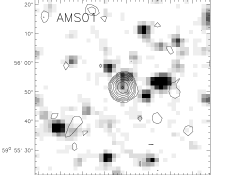
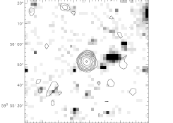
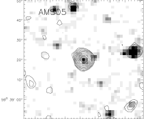
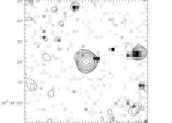
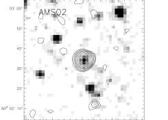
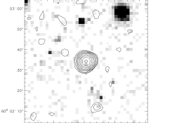
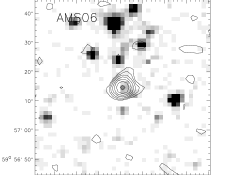
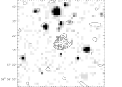
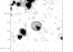
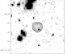
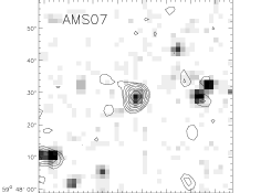
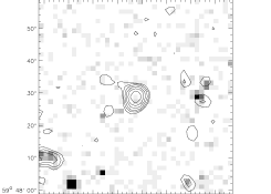
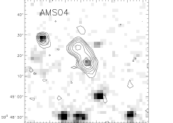
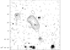
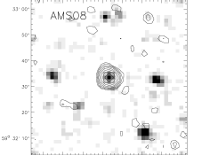
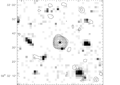
Figure 5: Radio contours overlayed over the 3.6-$\mu$m and R-band images for the sample (images from Condon et al., 2003; Fadda et al., 2004; Lacy et al., 2005). In each pair of overlays, the 3.6-$\mu$m image is on the left (with the name of the source) and the R-band on the right. Radio contours are plotted at -2$\sigma$,2$\sigma$ and subsequently at 2${}^{n/2}\sigma$ up to 2${}^{6}\sigma$, where $\sigma$ is the rms noise of the radio image ($\approx$ 23 $\mu$Jy). The gray scale has been chosen to overcome the high dynamical range and highlight faint objects. Faint grey pixels have values 3-times that of the noise.

Thus, to find all type-2 quasars (even the Compton thick ones), one requires a survey with a 2-10 keV flux limit of about $10^{-18}$ W m^-2 over a reasonably large area. Therefore, the SXDF survey (horizontal dotted line: Ueda et al. in prep.), which covers $\sim$1 deg² to this depth, should be able to find X-ray-selected Compton thick quasars. Comparing to the SWIRE depth, we can see that in the region of the SXDF, X-ray selection would be more sensitive than 24-$\mu$m selection, while still being able to find powerful type-2 quasars.

For Compton-thick objects, the X-ray selection function is almost flat for $0.5\raisebox{-2.58334pt}{$\,\stackrel{{\scriptstyle\raisebox{-0.60275pt}{$\textstyle<$}}}{{\sim}}\,$}z\raisebox{-2.58334pt}{$\,\stackrel{{\scriptstyle\raisebox{-0.60275pt}{$\textstyle<$}}}{{\sim}}\,$}2$. The redshift-distribution of Compton-thick type-2s in a survey deep enough to find them would therefore be dominated by the volume of the survey as a function of redshift and the evolution of the luminosity function. This means that X-ray surveys deep enough to be sensitive to Compton-thick type-2 quasars should find a wealth of $1\raisebox{-2.58334pt}{$\,\stackrel{{\scriptstyle\raisebox{-0.60275pt}{$\textstyle<$}}}{{\sim}}\,$}z\raisebox{-2.58334pt}{$\,\stackrel{{\scriptstyle\raisebox{-0.60275pt}{$\textstyle<$}}}{{\sim}}\,$}2$ objects. Coincidentally, this would be complementary to 24-$\mu$m surveys, as the mid-infrared surveys would struggle to find heavily obscured type-2s ($A_{\rm V}\raisebox{-2.58334pt}{$\,\stackrel{{\scriptstyle\raisebox{-0.60275pt}{$\textstyle>$}}}{{\sim}}\,$}50$), especially in the range around $z\sim 1.5$.

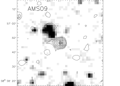
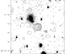
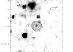
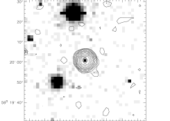
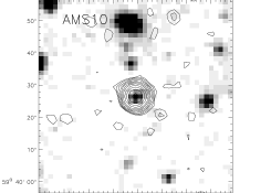
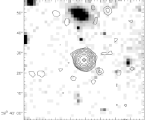
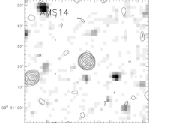
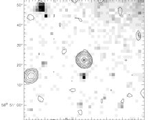
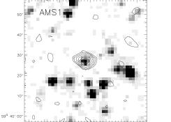
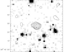
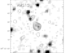
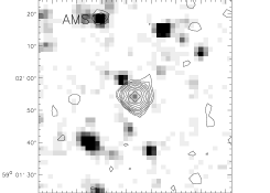
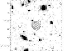
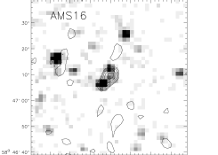
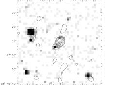
Figure 5: Continued

2.5 Dust type

A second-order effect for mid-infrared selection is the type of dust obscuring the AGN, which is particularly important in the range $1.2\raisebox{-2.58334pt}{$\,\stackrel{{\scriptstyle\raisebox{-0.60275pt}{$\textstyle<$}}}{{\sim}}\,$}z\raisebox{-2.58334pt}{$\,\stackrel{{\scriptstyle\raisebox{-0.60275pt}{$\textstyle<$}}}{{\sim}}\,$}1.8$ due to the varying depth of the silicate absorption feature. Figure 2 shows the ratio of transmission (see Figure caption), at observed 24-$\mu$m, for MW- and SMC-type dust. It shows clearly that for $z\raisebox{-2.58334pt}{$\,\stackrel{{\scriptstyle\raisebox{-0.60275pt}{$\textstyle<$}}}{{\sim}}\,$}3$ SMC-type dust will cause more absorption in the mid-infrared, in particular around 9.7-$\mu$m rest-frame ($z\sim 1.5$). Thus if the dust obscuring type-2s is more like the dust in the SMC than in the MW, then mid-infrared selection might perform slightly worse than expected from Figure 1. As mentioned earlier, the dust reddening type-1 quasars has been found to be more similar to SMC-dust, but that does not necessarily mean that the dust present in the obscuring torus is also SMC-type dust.

2.6 Orientation of the quasar

The analysis is mainly concerned with 24 $\mu$m selection of objects at $z\raisebox{-2.58334pt}{$\,\stackrel{{\scriptstyle\raisebox{-0.60275pt}{$\textstyle<$}}}{{\sim}}\,$}5$, so we are seeing light reprocessed by dust in the torus at a range of temperatures, $T=120-725$ K. We now use the results of a radiative transfer code by Granato & Danese (1994) to investigate the orientation dependence of observed 24-$\mu$m emission. In Figure 3 we quantify the fraction of the bolometric luminosity, $L_{\rm bol}$, seen at 24-$\mu$m as a function of redshift. For a pole-on unreddened source (necessarily a type-1), this fraction is approximately constant between $2\raisebox{-2.58334pt}{$\,\stackrel{{\scriptstyle\raisebox{-0.60275pt}{$\textstyle<$}}}{{\sim}}\,$}z\raisebox{-2.58334pt}{$\,\stackrel{{\scriptstyle\raisebox{-0.60275pt}{$\textstyle<$}}}{{\sim}}\,$}5$, while for an edge-on source (a type-2 with $A_{\rm V}\approx 50$), the fraction is similar to that of a type-1 and approximately constant in the range $2\raisebox{-2.58334pt}{$\,\stackrel{{\scriptstyle\raisebox{-0.60275pt}{$\textstyle<$}}}{{\sim}}\,$}z\raisebox{-2.58334pt}{$\,\stackrel{{\scriptstyle\raisebox{-0.60275pt}{$\textstyle<$}}}{{\sim}}\,$}4$. At higher values of $z$, the observed 24-$\mu$m corresponds to emitted wavelengths ($\raisebox{-2.58334pt}{$\,\stackrel{{\scriptstyle\raisebox{-0.60275pt}{$\textstyle<$}}}{{\sim}}\,$}5\mu$m) at which the dust is becoming progresively more opaque. Around $z\sim 1.5$ the silicate feature is seen in emission by the type-1 and absorption by the type-2, so the observed 24-$\mu$m emission is not a very good indicator of $L_{\rm bol}$. We can therefore conclude that 24-$\mu$m is a good indicator of bolometric luminosity at $2\raisebox{-2.58334pt}{$\,\stackrel{{\scriptstyle\raisebox{-0.60275pt}{$\textstyle<$}}}{{\sim}}\,$}z\raisebox{-2.58334pt}{$\,\stackrel{{\scriptstyle\raisebox{-0.60275pt}{$\textstyle<$}}}{{\sim}}\,$}4$ and, as shown in Figure 3, this result is not strongly dependent on the assumed size of the torus.

2.7 Summary

To summarise, we have discussed the advantages of mid-infrared selection over hard X-ray selection. For gas-to-dust ratios similar to those found in the Milky Way, X-ray selection is superior, and can probe further down the luminosity function. However, many AGN have gas-to-dust ratios significantly larger than the MW. We have seen in this section how type-2 quasars with $N_{\rm H}=5\times 10^{26}$ m${}^{-2}\times A_{\rm V}$ would naturally drop out of existing large-area X-ray samples without requiring extreme optical obscuration ($A_{\rm V}\raisebox{-2.58334pt}{$\,\stackrel{{\scriptstyle\raisebox{-0.60275pt}{$\textstyle>$}}}{{\sim}}\,$}20$ would be enough). We have seen that hard X-ray selected samples are in principle able to find even Compton-thick type-2s, but they require a combination of depth and area that is only just becoming available. We have also seen that dust-type is important, but mainly in the range $1\raisebox{-2.58334pt}{$\,\stackrel{{\scriptstyle\raisebox{-0.60275pt}{$\textstyle<$}}}{{\sim}}\,$}z\raisebox{-2.58334pt}{$\,\stackrel{{\scriptstyle\raisebox{-0.60275pt}{$\textstyle<$}}}{{\sim}}\,$}2$ (due to the 9.7-$\mu$m silicate absorption feature being more pronounced for certain dust types). Using the results of a radiative transfer code, we have also seen that (observed) 24-$\mu$m luminosity is a constant tracer of type-2 bolometric luminosity in the range $2\raisebox{-2.58334pt}{$\,\stackrel{{\scriptstyle\raisebox{-0.60275pt}{$\textstyle<$}}}{{\sim}}\,$}z\raisebox{-2.58334pt}{$\,\stackrel{{\scriptstyle\raisebox{-0.60275pt}{$\textstyle<$}}}{{\sim}}\,$}4$. Therefore, 24-$\mu$m selection is a natural starting place to look for the population of high-redshift type-2 quasars missing from X-ray surveys.

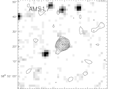
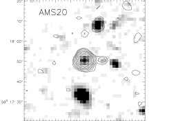
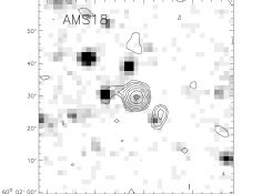
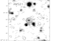
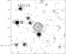
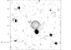
Figure 5: Continued

3 Selection Criteria

Our aim was to find the elusive high redshift type-2 population around the peak in the quasar activity, $z\raisebox{-2.58334pt}{$\,\stackrel{{\scriptstyle\raisebox{-0.60275pt}{$\textstyle>$}}}{{\sim}}\,$}2$ (e.g. Wolf et al., 2003), and for this we used the following selection criteria:

1. $S_{24~{}\mu\rm m}>300~{}\mu$Jy

2. $S_{3.6~{}\mu\rm m}\leq 45~{}\mu$Jy

3. $350~{}\mu\rm Jy\leq S_{1.4\rm~{}GHz}\leq 2$ mJy

3.1 Datasets

The work described in this paper was all done in the Spitzer Extragalactic First Look Survey (FLS). Three separate catalogues were cross-matched for the initial selection: the IRAC 3.6 $\mu$m (Lacy et al., 2005) and the MIPS 24 $\mu$m (Marleau et al., 2004; Fadda et al., 2006) from the Spitzer First Look Survey and the 1.4 GHz catalogue from the NRAO VLA (Condon et al., 2003). The flux limits used for 3.6 $\mu$m, 24 $\mu$m and 1.4 GHz were 20, 300 and 100 $\mu$Jy respectively.

Over the area with coverage in all three bands (3.8 deg²), the radio and 24-$\mu$m catalogues were matched, to select all sources detected at 24-$\mu$m and within the radio flux cuts. The chosen sources were then contrasted with the 3.6 $\mu$m catalogue, to obtain their flux densities in this IRAC channel. However, objects were not required to be detected at 3.6 $\mu$m to be kept in the candidate list. All matching was done with a 2.5 arcsec tolerance to allow for positional offsets between catalogues.

In addition, in this paper we use tabulate R-band magnitudes from data from the 4-m Mayall Telescope Kitt-Peak National Observatory (Fadda et al., 2004) and we also make use of a Westerbork Synthesis Radio Telescope deep survey at 1.4 GHz in the Spitzer First Look survey (Morganti et al., 2004). However, these two datasets were not used to select the candidate type-2 quasars.

3.2 Mid-infrared criteria

The mid-infrared criterion $S_{24~{}\mu\rm m}>300~{}\mu$Jy was chosen to select a flux-density-limited sample of active galaxies. At lower redshifts, a 24-$\mu$m selected sample would be dominated by starbursting galaxies, but combined with the 3.6-$\mu$m selection (which ensured high-redshift objects, see below), this 24-$\mu$m flux limit should yield powerful AGN. The $S_{24~{}\mu\rm m}>300$ $\mu$Jy criterion is the flux-density limit from a preliminary catalogue, and is actually a 7-$\sigma$ limit in the 24-$\mu$m final catalogue from the Spitzer FLS data (Marleau et al., 2004; Fadda et al., 2006). At $z=2$, this corresponds to an emitted 8-$\mu$m luminosity $L_{8~{}\mu\rm m}=10^{24.4}$ W Hz^-1. Assuming a typical type-1 SED (Rowan-Robinson, 1995), this is $L_{\rm B}=10^{23.2}$ W Hz^-1 or $M_{\rm B}=-23.8$. At $z=2$, the break in the quasar luminosity function, $L^{*}_{quasar}$, has a value of $M_{\rm B}=-25.7$ (Croom et al., 2004, with Pure Luminosity Evolution), so our 24-${\mu\rm m}$ selection will select quasars $\raisebox{-2.58334pt}{$\,\stackrel{{\scriptstyle\raisebox{-0.60275pt}{$\textstyle>$}}}{{\sim}}\,$}0.2~{}L^{*}_{quasar}$ at $z=2$, and more luminous quasars at higher redshifts. As explained in Section 2, the selection becomes more complicated at $z<2$ due to the silicate absorption, so we restrict our discussion to $z\geq 2$. The peak of the quasar activity occurred around $z\geq 2$ and by targeting the quasars around the “break” we are sensitive to the part of the population that contributes most of the luminosity density.

Quasars are considered as being type-2 if $A_{\rm V}\raisebox{-2.58334pt}{$\,\stackrel{{\scriptstyle\raisebox{-0.60275pt}{$\textstyle>$}}}{{\sim}}\,$}5$ (Simpson et al., 1999), and such an amount of extinction will make the observed near-infrared emission of type-2s much fainter than that of type-1s. The 3.6-$\mu\rm m$ criterion was therefore chosen to remove naked (type-1) quasars as well as lower redshift ($z\raisebox{-2.58334pt}{$\,\stackrel{{\scriptstyle\raisebox{-0.60275pt}{$\textstyle<$}}}{{\sim}}\,$}1.4$) type-2s. At $z\geq 2$ the detected 3.6-$\mu$m flux density corresponds to light emitted at $\lambda\leq$ 1.2 $\mu$m so dust extinction ensures that type-2 quasars are much fainter than type-1 quasars, even for a moderate $A_{V}$. Indeed, the $S_{3.6\mu\rm m}$ emission is likely to be dominated by starlight for $A_{V}\raisebox{-2.58334pt}{$\,\stackrel{{\scriptstyle\raisebox{-0.60275pt}{$\textstyle>$}}}{{\sim}}\,$}10$, and since light at 3.6-$\mu$m is dominated by the old stellar population, there will be an $S_{3.6\mu\rm m}-z$ correlation, analogous to the $K-z$ relation for radio galaxies (Jarvis et al., 2001b; Willott et al., 2003b). A typical host galaxy for a $z=2$ radio-quiet quasar is the progenitor of a $\sim 2L^{*}_{gal}$ (Kukula et al., 2001) galaxy in the local Universe, so we adapt the $K-z$ relation (which corresponds to $\sim 3L^{*}_{gal}$ hosts for radio galaxies) to $\sim 2L^{*}_{gal}$ hosts at 3.6-$\mu$m. To do this, we use the models of Bruzual & Charlot (2003) to form an elliptical galaxy at $z=10$, assign it a (stellar) mass and allow it to evolve passively. This allows us to predict the 3.6 $\mu$m flux as a function of redshift, for an elliptical galaxy of this given mass, and hence obtain a rough photometric redshift. The stellar mass of the galaxy was set to $3.8\times 10^{11}M_{\odot}$, and in Martínez-Sansigre et al. (2005) we quoted this as corresponding to $\sim 2L^{*}_{gal}$. If we assume a Salpeter IMF (Salpeter, 1955) and take $M_{\rm K}=-24.3$ from the fitting of Schechter functions by (Cole et al., 2001), then our assumed stellar mass translates to a $2.6L^{*}_{gal}$ galaxy. This is the host (elliptical) galaxy luminosity assumed to obtain the rough photometric redshifts in Martínez-Sansigre et al. (2005) and in this paper. The criterion $S_{3.6~{}\mu\rm m}\leq 45~{}\mu$Jy corresponds to a limiting photometric redshift $z_{\rm phot}\raisebox{-2.58334pt}{$\,\stackrel{{\scriptstyle\raisebox{-0.60275pt}{$\textstyle>$}}}{{\sim}}\,$}1.4$. This was chosen to target $z\sim 2$ type-2 quasars, while allowing for scatter in the crude photometric redshift estimation and filtering out type-1 quasars and low-redshift contaminants like radio galaxies.

The combination of these criteria is illustrated in Figure 4. It shows the observed spectral energy distributions of two $z=2$ quasars (model from Rowan-Robinson, 1995), a type-1 and a type-2 (the latter obscured by $A_{\rm V}=5$, dust model from Pei, 1992). A 2.6$L^{*}$ elliptical galaxy from Bruzual & Charlot (2003) is alos plotted at $z=1.4$, showing how the 3.6-$\mu$m criterion serves also as a crude photometric redshift cut.

3.3 Radio criterion

The radio selection criteria is added to ensure that the candidates are quasars rather than starburst galaxies. The 3.6-$\mu$m - 24-$\mu$m “colour” demanded by our criteria can be achieved by lower redshift ($z<1$) ultra luminous infrared galaxies (ULIRGs). For example, NGC 7714 would satisify these criteria if it were at $z=0.25-0.4$ (see Figure 4, SED from Brandl et al., 2004) and the more luminous ULIRG Arp 220 if it where at $z=0.5-0.7$. In the absence of AGN radio activity, the radio flux densities of such objects would follow the far-IR/radio correlation (, Condon 1992), and hence would have values of $S_{1.4~{}\rm GH}\sim 50$ (for ULIRGs at $z\sim 0.3$) and $500~{}\mu$Jy (for more powerful ULIRGs at $z\sim 0.6$).

To avoid such starburst contaminants, we chose a lower limit on $S_{1.4~{}\rm GHz}$ which also excludes higher-redshift (submillimetre-selected) starburst galaxies without the benefit of strong gravitational lensing (e.g. Chapman et al., 2005). For a $z\sim 0.6$ ULIRG to have $S_{1.4~{}\rm GH}\geq 350~{}\mu$Jy, it would require a far-infrared luminosity of $L_{\rm FIR}\raisebox{-2.58334pt}{$\,\stackrel{{\scriptstyle\raisebox{-0.60275pt}{$\textstyle>$}}}{{\sim}}\,$}1\times 10^{12}$ $L_{\odot}$. Objects with this far-infrared luminosity are rare in space-density (Sanders & Mirabel, 1996), and the comoving volume probed at $z\sim 0.6$ by 3.8 deg² is such that $\raisebox{-2.58334pt}{$\,\stackrel{{\scriptstyle\raisebox{-0.60275pt}{$\textstyle<$}}}{{\sim}}\,$}1$ contaminants would be expected in our sample.

An upper limit on $S_{1.4~{}\rm GHz}$ was also used to filter out the radio-loud objects, whose extended jets might complicate interpretation. The radio flux-density cut introduced here will select the radio-bright end of the radio-quiet quasar population (Cirasuolo et al., 2003), so these objects can be described as radio-intermediate. In addition, the $S_{3.6\mu\rm m}$ criterion includes objects without IRAC detections which we expect to have the highest redshifts. Since the 24-$\mu$m positions are accurate to $\sim 1$ arcsec, the FLS radio positions (Condon et al., 2003), accurate to $\sim 0.5$ arcsec, were also better for spectrosocopic follow-up.

Name	RA	Dec	Date	Airmass	PA	Slit
	(J2000)		Observed		/deg	/arcsec
AMS01	17 13 11.17	+59 55 51.5	15/07/04	1.17	103	1.5
AMS02	17 13 15.88	+60 02 34.2	14/07/04	1.37	149	2.0
AMS03	17 13 40.19	+59 27 45.8	14/07/04	1.17	114	1.5
AMS04	17 13 40.62	+59 49 17.1	14/04/05	1.18	36	2.0
AMS05	17 13 42.77	+59 39 20.2	14/07/04	1.47/1.56[1]	98	2.0
AMS06	17 13 43.91	+59 57 14.6	13/07/04	1.19	120	2.0
AMS07	17 14 02.25	+59 48 28.8	16/07/04	1.22	19	1.5
AMS08	17 14 29.67	+59 32 33.5	15/07/04	1.32	128	1.5
AMS09	17 14 34.87	+58 56 46.4	15/07/04	1.17	111	1.5
AMS10	17 16 20.08	+59 40 26.5	14/07/04	1.20	114	1.5
AMS11	17 18 21.33	+59 40 27.1	16/07/04	1.19	76	1.0
AMS12	17 18 22.65	+59 01 54.3	15/07/04	1.16	150	1.5
AMS13	17 18 44.40	+59 20 00.8	14/04/05	1.16	186	2.0
AMS14	17 18 45.47	+58 51 22.5	13/07/04	1.20	105	2.0
AMS15	17 18 56.93	+59 03 25.0	15/04/05[2]	-	-	-
AMS16	17 19 42.07	+58 47 08.9	16/07/04	1.25	141	2.0
AMS17	17 20 45.17	+58 52 21.3	15/04/05	1.27	117	1.5
AMS18	17 20 46.32	+60 02 29.6	13/07/04	1.40	133	2.0
AMS19	17 20 48.00	+59 43 20.7	14-15/04/05	1.17/1.17	170/185	2.0
AMS20	17 20 59.10	+59 17 50.5	14/07/04	1.22	160	2.0
AMS21	17 21 20.09	+59 03 48.6	15/04/05	1.20	84	1.5

Table 1: Summary of the spectroscopic observations. Most of the objects were observed in July 2004, and the spectroscopy was completed in April 2005. The objects were all observed with airmass $<1.5$ (except AMS05), with good seeing (in the range 0.7-1.0 arcsec). As described in Section 4, the position angles (PAs) of the slit were generally chosen to go through any other radio source in the field, or any bright 3.6 $\mu$m source, to help the astrometry and identification. In some cases neither were available, or the airmass was high, so the PA was chosen to match the parallactic angle and therefore minimise dispersion of the blue light. ^[1]AMS05 was observed twice on the same night, at different airmasses. ^[2]AMS15 was targetted in the April 2005, but the position used was slightly wrong ($\sim 0.8$ arcsec) and therefore we do not consider it to have been observed.

The two simple infrared criteria together with radio selection were chosen over an IRAC colour requirement because the latter criterion would have selected type-2s with a narrow range in $A_{\rm V}$ and $z$. Our three criteria represent a simple way of selecting type-2 quasars and allow the modelling necessary to estimate the quasar fraction at high redshift (Martínez-Sansigre et al., 2005).

After these selection criteria, we were left with 21 candidate high-redshift type-2 quasars (see Table 2), which were followed up spectroscopically (as described in Section 4). Note that all our candidates were originally selected from the preliminary 3.6 and 24 $\mu$m catalogues, but have had their fluxes slightly revised and the flux densities quoted are the final ones. This explains why two candidates are slightly outside the selection boundaries. We also note that although the R-band (Vega) magnitudes are not part of our selection criteria, they are consistent with optically obscured quasars in high-redshift host galaxies. At $z=1.4$, our model elliptical galaxy would have $m_{\rm R}=23.3$.

4 Observations and Data Reduction

The 21 candidates were observed with both arms of the ISIS instrument at the William Herschel Telescope in July 2004 and April 2005 (see Table 1). Low-resolution long slit spectroscopy was performed across the entire visible band (3200 Å  to 9300 Å) using the gratings R158B and R158R, and the EEV12 and Marconi detectors. The 6100 Å  dichroic was used in July 2004, while in April 2005 we used the new 5300 Å  dichroic. Using slit widths of 1.5-2.0 arcsec, we obtained spectral resolutions of 12-16 Å  in both arms. Bias, flat, arc, sky-flat and standard-star frames were all taken at the beginning and end of the night to ensure reasonable callibration.

Name	RA	Dec	$S_{24\mu\rm m}$	$S_{1.4\rm GHz}$	$S_{3.6\mu\rm m}$	$S_{4.5\mu\rm m}$	$m_{\rm R}$	$z_{\rm phot}$	$z_{\rm spec}$
	(J2000)		/ $\mu$Jy	/ $\mu$Jy	/ $\mu$Jy	/$\mu$Jy
AMS01	17 13 11.17	+59 55 51.5	536	490	25.0	30.0	25.1	2.1
AMS02	17 13 15.88	+60 02 34.2	294	1184	44.5	61.0	25.3	1.4
AMS03	17 13 40.19	+59 27 45.8	500	1986	16.0	28.0	24.4	3.1	2.698[1]
AMS04	17 13 40.62	+59 49 17.1	828	536	18.0	22.0	22.96	2.8	1.782
AMS05	17 13 42.77	+59 39 20.2	1769	1038	34.7	61.4	25.2	1.7	2.017
AMS06	17 13 43.91	+59 57 14.6	969	444	$<$20	$<$25	$\geq$25.3	$\geq$2.5	1.76[2]
AMS07	17 14 02.25	+59 48 28.8	503	354	37.9	47.8	24.7	1.5
AMS08	17 14 29.67	+59 32 33.5	792	655	41.6	46.3	22.48	1.4	1.979
AMS09	17 14 34.87	+58 56 46.4	685	426	25.2	$<$25	$\geq$25.3	2.1
AMS10	17 16 20.08	+59 40 26.5	338	1645	39.2	44.7	24.1	1.5
AMS11	17 18 21.33	+59 40 27.1	442	356	32.4	55.6	24.7	1.7
AMS12	17 18 22.65	+59 01 54.3	518	946	25.24	$<$25	23.77	2.0	2.767
AMS13	17 18 44.40	+59 20 00.8	4196	1888	24.7	49.1	22.89	2.1	1.974[3]
AMS14	17 18 45.47	+58 51 22.5	937	469	8.0	15.0	23.67	4.6	1.794
AMS15	17 18 56.93	+59 03 25.0	371	440	16.0	16.0	$\geq$25.3	3.0	Not Observed[4]
AMS16	17 19 42.07	+58 47 08.9	788	390	18.0	21.0	23.07	2.8	4.169
AMS17	17 20 45.17	+58 52 21.3	1134	615	10.0	15.0	23.80	3.9	3.137[1]
AMS18	17 20 46.32	+60 02 29.6	925	390	$<$20	$<$25	23.53	$\geq$2.5	1.017
AMS19	17 20 48.00	+59 43 20.7	1433	822	$<$20	26.9	$\geq$25.3	$\geq$2.5	2.25[2]
AMS20	17 20 59.10	+59 17 50.5	492	1268	45.2	64.9	23.80	1.4	[5]
AMS21	17 21 20.09	+59 03 48.6	720	449	25.2	38.6	24.2	2.1

Table 2: Basic data on the 21 type-2 quasars in our sample. The J2000.0 positions are from the Spitzer FLS radio catalogue (Condon et al., 2003). The MIPS 24-$\mu$m flux density $S_{24\mu\rm m}$ is obtained by point spread function (PSF) fitting (Marleau et al., 2004) as all objects (except AMS16) are point sources at the $\sim 6$ arcsecond resolution of the MIPS observations, with positional errors $\sim 1$ arcsecond. It has a typical error of $\pm 10-15$%. The 1.4-GHz flux density is the peak value (in $\mu$Jy per beam) from the radio catalogue. The IRAC 3.6- and 4.5-$\mu$m flux densities are measured in 5-arcsec-diameter apertures (Lacy et al., 2005) and have typical errors of $\pm 10$%. The R-band magnitudes are measured using a 3-arcsecond diameter aperture from the images of the 4-m Mayall Telescope Kitt-Peak National Observatory (Fadda et al., 2004), with typical errors of 0.03 for objects with magnitude 22-23, 0.10 for objects with 23-24 and 0.25 mags for those with magnitudes of 25. ^[1] These objects have redshifts identified from a single line, which we identified as Lyman-$\alpha$: in AMS03, from the amount of structure in the line, and in AMS17 from the fainter continuum blueward of the line. ^[2] These two objects have redshifts from Spitzer-IRS spectroscopy from Weedman et al. (2006), who give two values for the redshifts. Here we show the mean of the two values. ^[3] This object was observed with Spitzer-IRS by Yan et al. (2005) who measured a redshift of $z=2.1\pm 0.1$ in good agreement with our value. ^[4] As explained in Table 1, AMS15 has not really been observed spectroscopically.^[5] AMS20 Shows faint red continuum but no emission lines. Note there were errors in the redshifts of AMS14 and AMS18 presented in Table 1 of Martínez-Sansigre et al. (2005) and these have been corrected here, together with minor corrections to several other redshifts.

The slit was placed on the radio positions, without optical identification, by “blindly” offsetting from a nearby guide star (e.g. Rawlings et al., 1990). Whenever another radio source was in the field, the slit angle was chosen to go through the source as well as our candidate. When no other radio sources were available, bright sources from the IRAC 3.6-$\mu$m catalogue were placed in the slit. This ensured multiple objects were detected in the slit, improving the astrometry and identification of our sources in the 2-D spectra. At high airmasses ($\sim 1.4-1.5$) we observed the objects with slit position angles (PAs) close to the parallactic angle, to minimise atmospheric dispersion of the blue light. Each object was observed for 30 minutes with a 1-2 arcsec slit width, with one 1800 second exposure in the blue arm and two 900 second exposures in the red arm.

The spectra were all reduced using the iraf package twodspec longslit. The wavelength calibration was performed using CuAr+CuNe lamps and flux callibration was obtained from appropriate spectrophotometric stars. The two red frames for each object were reduced separately and then combined to remove cosmic rays. The 1D spectra were extracted separately for the blue and the combined red frames, using the task apsum. The resulting one-and two-dimensional spectra are plotted in Figure 6.

AMS01 The 3.6 $\mu$m image of this object shows it to be visible, although possibly confused with a galaxy just to the North (N) of it (see Figure 5). However, in the R-band image we see our target is distinguishable as an extremely faint galaxy. The two images clearly show the very red colour of AMS01. There was another radio source of similar flux East (E) of AMS01 and so a position angle (PA) of 103 degrees was chosen to go through both sources. The spectrum of AMS01 was completely blank in a 30-minute exposure..

AMS02 In this case, our target is clearly visible in the IRAC image, but is only just detected in the R-band. The PA was chosen to go through another radio source, 45 arcsec SE of AMS02. The spectrum of our target was once again completely blank in a 30-minute exposure.

AMS03 Here we see another possible source of confusion in the 3.6 $\mu$m image, but the R-band image shows our source to be very faint but distinct from the brighter source SW of it. There is a nearby radio source which is confused in the WSRT images (see Section 8). Here the PA was chosen to go through this other radio source 18 arcsec E-SE of AMS03. The two-dimensional spectrum shows a faint, double, spatially-extended line ($\sim$ 1.6 arcsec once deconvolved from the seeing), which we identify as Ly $\alpha$ (the redward line is not N V). The spectrum shows quite a lot of structure (see Figure 6): there are two Ly-$\alpha$ lines, one at 4481 Å  and the other at 4512 Å. The redward line has a full-width half maximum (FWHM) of $\sim$ 500 km s^-1, while the blueward line has a hint of absorption in the spatial centre, and has a greater FWHM ($\sim$ 1400 km s^-1) but still narrow enough to qualify as a type-2 quasar. A possible interpretation is that the type-2 quasar resides in a Ly-$\alpha$ halo, and there is a large difference in systemic velocity for the quasar and the halo (or the halo is collapsing, leading to an additional redshift). Another possibility is associated absorption - this is present in small radio sources (van Ojik et al., 1997).

AMS04 This object is very faint at 3.6 $\mu$m (18 $\mu$Jy) but reasonably bright in R-band ($m_{\rm R}=$23). The radio emission around AMS04 is extended towards the NE. There is another distant radio source, identified at both 3.6 $\mu$m and R-band further to the east. This is possibly associated with another extremely faint galaxy about 10 arcsec away, although the radio and optical positions of the adjacent radio source and the faint galaxy do not match perfectly. We placed the slit to go through both AMS04 and the other radio source. AMS04 shows strong continuum, a spatially extended (and bright) Ly $\alpha$ as well as C III], N II] and C II] lines but nothing was seen associated with the extended radio emission. The Ly $\alpha$ line has an angular size of $\sim 5.5$ arcsec. This object has a redshift of 1.782, with all the redshifts from individual lines agreeing well (see Table 3). The fact that this object is not that faint in R-band is due to the continuum and narrow-lines at the red end of the spectrum.

AMS05 Here we see again a source which is relatively bright at 3.6 $\mu$m (34 $\mu$Jy) compared to R-band ($m_{\rm R}=$25.2). The IRAC image is quite crowded and there is the danger of confusing sources, but we can see in the R-band that the radio position falls on a faint galaxy. This object showed an interesting spectrum: C IV is actually as strong as Ly $\alpha$, and He II is also detected, but there is no continuum in the blue or red arm. All lines are unresolved, and the weakness of the Ly $\alpha$ may be due to it falling in the blue end of the spectrum while having been observed at a high airmass (see Table 1) and away from the parallactic angle.

AMS06 This target is just about visible in the 3.6 $\mu$m images, but it is not bright enough to make it to the IRAC catalogue. It is undetected in the R-band. A PA of 120^∘was chosen to go through the “semi-major axis” of the marginally-resolved radio source. The spectrum was blank at the location of the target source. This could be due to the entire galaxy being very dusty and therefore faint in the optical and even the infrared (see the Section 9) or it could be a very high redshift source. Recently a redshift of 1.76 has been obtained from silicate absorption and PAH emission with Spitzer IRS (Weedman et al., 2006), confirming this is a very dusty system at high redshift.

AMS07 AMS07 is quite a red object (within our sample) in that the 3.6 $\mu$m is relatively bright, whereas the R-band is very faint. There is another radio source 56 arcsec SW of the target, so the slit (with PA 19^∘) was made to go through both radio sources. The spectrum was blank at the target position.

                           

                           

                           

Figure 6: Optical spectra of objects in the sample which showed emission lines. The emission lines from which the redshifts were obtained are labelled, while tentative identifications of lines which have not used for the redshifts are labelled with a question mark. The corresponding two-dimensional spectra are shown underneath the one-dimensional ones as a visual help to find the emission lines. They have approximately the same scale in the horizontal direction as the one-dimensional spectra. The grey scale has been chosen to bring out low signal-to-noise lines and can lead to visual artefacts such as the strange change in continuum strength of AMS08. For the two objects observed in April 2005 (AMS04 and AMS13), the pixel scale in the dispersion axis was not the same for the blue and red arms, and so the two-dimensional spectra are not combined, just overlayed on each other. Particularly strong residual sky lines have been labelled in the one-dimensional spectra and are clearly visible in the two-dimesional ones. In AMS04, the sky lines are close to the N II] and C II] lines, making these two lines hard to detect in the grey scale image. The reader is assured that these two lines are detected and are not due to the residual sky lines.

                                                                

Figure 6: Contined.

AMS08 Here we have a relatively bright source for our sample, both in the IRAC and R bands. A faint (slightly extended) radio source, 18 arcsec SE of our source, was visible in the radio images. The slit was made to go through both this source and our target. AMS08 appears in the spectrum, showing Ly $\alpha$ ($\sim$ 3.7 arcsec wide after deconvolving from the seeing), C IV and He II and blue continuum.

AMS09 This is a faint source at 3.6 $\mu$m and is undetected in R-band. The 3.6 $\mu$m image shows only one infrared ID for our radio source, but the R-band image shows there might be a serious confusion issue, as there are several faint sources near the radio position. There were two other radio sources in the field, one close to the N (visible in Figure 5) and one E. We chose to place the slit through the eastern radio source (41 arcsec away) and the PA angle (119 deg) is actually appropriate to try and catch several of the possible optical IDs. There is barely a hint of continuum from AMS09 in the red two-dimensional spectrum and no hint of the other source.

AMS10 AMS10 is a relatively bright source in the IRAC bands, and has $m_{\rm R}=$24.1. The 3.6 $\mu$m source is actually confusing two R-band sources, but the radio position is clearly associated to only one of the R-band galaxies. There were no other radio sources in the field, so we chose the PA to match the parallactic angle. The 2D spectrum of AMS10 is blank.

Name	$z$	Line	$\lambda_{\mathrm{r}est}$	$\lambda_{\mathrm{o}bs}$	FWHM	Flux	log${}_{10}L_{\rm line}$	Error in flux
			/Å	(Å)	/km s-1	/W m-2	/W	/%
AMS03	2.698 $\pm$ 0.009	Ly $\alpha$	1216	4481	1400	$1.22\times 10^{-19}$	35.86	20
		Ly $\alpha$	1216	4512	550	$3.69\times 10^{-20}$	35.34	18
AMS04	1.782 $\pm$ 0.001	Ly $\alpha$	1216	3382	1800	$5.01\times 10^{-19}$	36.04	12
		C III]	1909	5311	1450	$1.02\times 10^{-19}$	35.35	21
		N II]	2142	5963	2550	$1.16\times 10^{-19}$	35.40	20
		C II]	2326	6467	1250	$8.59\times 10^{-20}$	35.27	28
AMS05	2.017 $\pm$ 0.006	Ly $\alpha$	1216	3658	1250	$1.32\times 10^{-19}$	35.59	38
		C IV	1549	4681	1000	$1.16\times 10^{-19}$	35.53	18
		He II	1640	4952	500	$3.16\times 10^{-20}$	34.97	41
AMS08	1.979 $\pm$ 0.004	Ly $\alpha$	1216	3622	1900	$5.05\times 10^{-19}$	36.15	15
		C IV	1549	4622	1400	$4.49\times 10^{-20}$	35.10	23
		He II	1640	4877	900	$2.30\times 10^{-20}$	34.81	35
AMS12	2.767 $\pm$ 0.005	Ly $\alpha$	1216	4586	650	$4.41\times 10^{-19}$	36.45	17
		C IV	1549	5824	1150	$3.50\times 10^{-20}$	35.35	25
		He II	1640	6181	1100	$2.22\times 10^{-20}$	35.15	26
AMS13	1.974 $\pm$ 0.003	Ly $\alpha$	1216	3613	1650	$9.88\times 10^{-19}$	36.44	12
		C IV	1549	4611	1300	$1.67\times 10^{-19}$	35.67	20
AMS14	1.794 $\pm$ 0.001	Ly $\alpha$	1216	3398	1500	$3.69\times 10^{-19}$	35.91	18
		C IV	1549	4326	600	$5.61\times 10^{-20}$	34.92	21
AMS16	4.169 $\pm$ 0.002	Ly $\alpha$	1216	6288	1050	$3.19\times 10^{-19}$	36.73	12
		N V	1240	6406	2050	$1.56\times 10^{-19}$	36.42	28
		C IV	1549	8009	2050	$2.69\times 10^{-19}$	36.66	16
AMS17	3.137 $\pm$ 0.002	Ly $\alpha$	1216	5031	1200	$2.89\times 10^{-19}$	36.40	16
AMS18	1.017 $\pm$ 0.004	C II]	2326	4680	1400	$8.19\times 10^{-20}$	34.65	25
		Mg II	2798	5652	3500	$1.14\times 10^{-19}$	34.79	44
		[O II]	3727	7527	2200	$1.12\times 10^{-19}$	34.79	27

Table 3: Table of emission line properties of the 10 objects with spectroscopic redshifts from our optical spectroscopy. The lines were fitted with gaussians to find $\lambda_{\mathrm{o}bs}$, FWHM, and the flux. For objects with several lines, the error quoted is the square root of the average variance. For objects with only one line, the error is assumed to be dominated by the fitting of a gaussian to the line. This in turn is dominated by the spectral resolution and the seeing. In two cases (AMS14 and AMS18) an error in wavelength calibration led to incorrect identification of lines and redshifts in Martínez-Sansigre et al. (2005). The error in flux (and luminosity) is the sum in quadrature of the photometric error (typically 10%), the error from the slit (typically 5%) and the uncertainty in the continuum. The FWHM is deconvolved by subtracting in quadrature the seeing from the observed size of the emission line. For lines with errors $>20$% the measurements of the FWHM are not reliable, and the presence of broad lines (e.g. Mg II in AMS18) is therefore not significant.

AMS11 This is another quite red source, relatively bright at 3.6 $\mu$m and faint in R-band. There are no other radio sources near but the radio emission seems to be slightly extended in the E direction, so we chose the PA so the slit would go through it. AMS11 was not detected by ISIS.

AMS12 Here we have a faint source in all bands. The PA was chosen to go through a radio source 50 arcsec SE of our target. The spectrum of AMS12 shows several emission lines: Ly $\alpha$ (spatially unresolved), C IV and He II (see Table 3) and faint continuum.

AMS13 AMS13 is a point-like radio source, and is quite faint at 3.6 $\mu$m, so we matched the PA to the parallactic to minimise dispersion of the blue light (even though the airmass, 1.16, was not particularly high). In the 2D spectrum, however, it is very bright, showing spatially extended Ly $\alpha$ and C IV lines ($\sim$ 4.3 and 3.5 arcsec wide respectively) as well as continuum. The continuum explains why it is not that faint in the R-band. The optical spectra show AMS13 is at a redshift of 1.974, and Yan et al. (2005) find a redshift of 2.1 $\pm$ 0.1 from the silicate absorption feature in their Spitzer-IRS spectroscopy, in agreement with our redshift.

AMS14 This source is extremely faint in the IRAC bands (8 $\mu$Jy at 3.6 $\mu$m) making us expect this to be a very high redshift source. A PA of 105^∘was chosen to go through another faint radio source 10 arcsec E of our target. The spectrum, however, shows a very strong (and spatially resolved) Ly $\alpha$ line ($\sim$ 1.6 arcsec wide) as well as C IV at a redshift of $z=1.794$. A mistake in an early wavelength calibration led us to mis-identify the lines and the redshift reported in Martínez-Sansigre et al. (2005) is incorrect.

AMS15 This is another very faint source at 3.6 $\mu$m and undetected in R-band. This is a good candidate for a high-redshift type-2 quasar. However we used a slightly wrong position (the one published in Martínez-Sansigre et al. (2005) is off by $\sim$0.8 arcsec) for follow-up spectroscopy. For this reason we do not consider this object to have been observed.

AMS16 AMS16 is very faint in the IRAC bands, although it is not extremely faint in R-band ($m_{\rm R}=23.07$). It has an extended radio structure, whose central position matches the optical and IR positions. However, the extended emission matches very well two galaxies next to the source, and in the 24-$\mu$m image the three sources are confused, and have a similar structure to the radio emission. There is the possibility that the two foreground galaxies might be lensing AMS16 (see Figure 5). Two factors therefore influenced the choice of PA in this case. First, the radio emission around AMS16 is extended in the SE to NW direction (diagonally, possibly due to the two galaxies). In addition, there is a radio loud ($S_{1.4~{}\rm GHz}=$21.6 mJy) type-1 quasar about an arcmin NW. By good fortune, the same angle is required to get the slit through the ‘semi-major axis’ of the extended radio emission, the brighter foreground galaxy and the type-1 quasar. We found Ly $\alpha$ ($\sim$ 2.7 arcsec), N V ($\sim$ 1 arcsec) and C IV (spatially unresolved) in AMS16, indicating a redshift of $z=4.169$. The emission lines of AMS16 are all strong, which explains why it is not that faint in the R-band. To the NW of AMS16, 58 arcsec away, we found a radio-loud type-1 quasar, at redshift $z=3.785$ (see Figure 7).

AMS17 This is another faint source in the IRAC bands, suggesting a high redshift, although the R-band is not particularly faint for this sample, and the images show the optical/IR positions match perfectly the centre of the radio emission, with no possible sources of confusion nearby. The slit PA was chosen to go through another object, about 59 arcsec SE of our target. AMS17 is indeed at high-redshift, as it shows one narrow line in the blue spectrum (which we identify as Ly $\alpha$ at $z=3.137$) and faint continuum redwards of the line. The Ly $\alpha$ line is extended $\sim$ 1.6 arcsec wide in the spatial direction, once the seeing is deconvolved.

AMS18 Here is a source which is undetected in the IRAC catalogues, which suggests a high redshift. The PA was chosen to go through a bright radio source 57 arcsec South-East. The 2D spectrum shows AMS18 has several faint emission lines, which we identify as C II], Mg II and [O II] at $z=1.017$, so it is at a lower redshift than first expected from the crude photometric redshift. Note the weakness of the [O II] line, which suggests a faint AGN rather than something similar to a radio galaxy. The same wavelength calibration error discussed for AMS14 led to the redshift of AMS18 being incorrect in Martínez-Sansigre et al. (2005). The emission lines are those of an AGN, so this is probably a less-luminous quasar possibly hosted by a small galaxy, which is how it made it through our selection criteria. It is however, difficult to judge whether the lines are spatially extended, due to the low SNR.

AMS19 The PA was chosen to be identical to the parallactic angle, as it is very faint in the near-infrared and the radio emission of AMS19 is point-like. This could mean a high redshift, so we tried to maximise the blue light received. Indeed, in the two-dimensional AMS19 does not even show faint continuum. However it was also observed by Weedman et al. (2006) with Spitzer IRS and is found to be at $z=2.25$ from it’s PAH and Silicate features.

AMS20 This is a relatively bright source for our sample, and so is not expected to lie at a particularly high redshift. The slit was placed at an angle so it would go through two fainter radio sources NW of AMS20 (19 and 55 arcsec away). The spectrum of AMS20 shows faint red continuum but no lines to allow us to obtain a redshift. Further study is required to determine whether this is a very bright high-redshift type-2, or more similar to AMS18, a faint, lower-redshift object. The lack of lines suggests $z\sim 1.3-1.6$.

AMS21 The last source in our sample is relatively faint in at 3.6 $\mu$m and R-band. In this case, the PA was chosen to go through a fainter radio source about 25 arcsec E of the target. However, neither AMS21 or the other radio source have been detected in the optical spectrum.

5 Type-2 Spectra

Approximately half of the objects (10 out of 21) showed narrow emission lines and sometimes continuum (see Figure 6). Ly $\alpha$ with full-width half maximum (FWHM) $\raisebox{-2.58334pt}{$\,\stackrel{{\scriptstyle\raisebox{-0.60275pt}{$\textstyle<$}}}{{\sim}}\,$}2000~{}\rm~{}km~{}s^{-1}$ was found in nine objects (with a redshift range $1.78\leq z\leq 4.17$) and high excitation lines such as CIV (1549 Å) or HeII (1640 Å) were also found in several objects (see Table 3). In two cases (AMS03 and AMS17) we only found one emission line, which was taken to be Ly $\alpha$ by virtue of its extreme equivalent width, blue-absorbed line profile and lack of other lines supportive of alternative identifications. The Ly $\alpha$ line of AMS03 is particularly spatially-extended. One object, AMS18, proved to be at $z=1.02$, lower than expected from our selection criteria. AMS18 is still an AGN, so there is still no evidence of pure-starburst contamination. Only one object showed (very faint) continuum and no lines: AMS20. As mentioned in Section 4, it will require more study to determine whether this object is similar to AMS18, is at $1.3\raisebox{-2.58334pt}{$\,\stackrel{{\scriptstyle\raisebox{-0.60275pt}{$\textstyle<$}}}{{\sim}}\,$}z\raisebox{-2.58334pt}{$\,\stackrel{{\scriptstyle\raisebox{-0.60275pt}{$\textstyle<$}}}{{\sim}}\,$}1.7$, or is at a higher-redshift object. If this object were a contaminant, like a $z\sim 0.5$ ULIRG, it would have shown stronger continuum and the [O II] 3727 Å line. It is important to insist on how faint our sources are: all objects, even those with emission lines in the R-band or showing some continuum, have $\rm m_{\rm R}\geq 22.5$ (Vega), and most have $\rm m_{\rm R}\geq 23$. The rest of the objects show blank spectra, confirming that there are no low-redshift contaminants in our sample. A 2.6$L^{*}$ elliptical at $z=1.4$ would have a continuum flux density of $1\times 10^{-21}$ W m^-2 Å^-1, at the limit of our sensitivity. AMS20, with faint red continuum, is therefore consistent with having an elliptical host galaxy, and being somewhere in the spectroscopic desert.

The nature of the blank-spectrum objects is discussed further in Section 9, but we see that their blank optical spectra are consistent with host ellipticals at $z\raisebox{-2.58334pt}{$\,\stackrel{{\scriptstyle\raisebox{-0.60275pt}{$\textstyle>$}}}{{\sim}}\,$}1.4$. If 24-$\mu$m flux density is a good tracer of narrow emission line strength, then we expect all our sources to have detectable Ly $\alpha$ lines if they lie at $z\geq 1.7$. In addition, the C IV (1549Å) line is detected in six out of the nine objects with Ly $\alpha$, and in the composite spectrum (see Section 7) it has 36% of the flux of Ly $\alpha$. Hence, some objects in the spectroscopic desert should also have detectable C IV lines. The two blank objects brightest at 24-$\mu$m have redshifts from Spitzer-IRS in the same range as the rest of the optical spectra, where we should have seen Ly $\alpha$. This suggests that at least some of the blank objects are at redshifts high enough to have narrow emission lines in the optical band, and that their spectra are blank for another reason. This reason could be that they have weaker emission lines, but they would have to be significantly weaker than those of the narrow-line objects, despite having similar 24-$\mu$m fluxes. Another alternative, is that the narrow emission line region is itself obscured, as has proven to be the case from the Spitzer spectroscopy of AMS06 and AMS19.

6 Crude Photometric Redshifts

As discussed in Section 3, for $A_{\rm V}\raisebox{-2.58334pt}{$\,\stackrel{{\scriptstyle\raisebox{-0.60275pt}{$\textstyle>$}}}{{\sim}}\,$}10$ the 3.6-$\mu$m flux density should be dominated by light from the host galaxy’s old stellar population. We estimated crude “photometric” redshifts for the entire sample by assuming the host galaxies to be the progenitors of present day massive elliptical galaxies. These galaxies were taken from the models of Bruzual & Charlot (2003), formed at $z=10$ in a single starburst, with a Salpeter IMF (Salpeter, 1955) and a stellar mass of $3.8\times 10^{11}M_{\odot}$. Such host galaxies would become 2.6 $L^{*}$ galaxies in the local $K$-band luminosity function (Cole et al., 2001). The justification for such an assumption is that radio-loud galaxies show a $K-z$ Hubble diagram consistent with such massive host galaxies ($\sim 3L^{*}$ Jarvis et al., 2001b; Willott et al., 2003b) and evidence points to the host galaxies of $z\sim 2$ radio-quiet quasars being $\sim 2L^{*}$ ellipticals (Kukula et al., 2001).

Figure 7: The spectrum of the type-1 quasar observed at the same time as AMS16.

The scatter in true host luminosity means that individually, the photometric redshifts are not necessarily close to the spectroscopic redshift, but they agree on average for 10 of the 12 objects. There are two cases (AMS14 and AMS18) in which the photometric redshift is clearly overestimated. There are two possible explanations for this: a host galaxy which is smaller than the progenitors of $\sim 2-3L^{*}$ ellipticals, and so our mass is an overestimate, or a star-forming host-galaxy, in which case our elliptical galaxy template is not appropriate. For the objects that have spectroscopy, the mean and median values of $z_{\rm phot}$ are 2.75 and 2.65 respectively while the mean and median spectroscopic redshifts are 2.33 and 2.00 (2.29 and 2.00 if the Spitzer-IRS are included): this represents reasonable agreement for such a simple photometric redshift estimation and gives us some confidence that we can estimate how many objects that remained unobserved or had blank optical spectra are at $z\geq 2$. To bring the median $z_{\rm phot}$ to the value of the median $z_{\rm spec}$ one would have to change the mass of the elliptical to $2.9\times 10^{11}M_{\odot}$, which would correspond to the progenitor of a $\sim 2L^{*}$ elliptical galaxy instead of $\sim 2.6L^{*}$. This would also bring the mean $z_{\rm phot}$ close to the mean $z_{\rm spec}$. The fact that, for the objects with emission lines, the “photometric” redshifts are roughly in agreement with the spectroscopic ones, suggests the host galaxies are the progenitors of massive ellipticals ($\raisebox{-2.58334pt}{$\,\stackrel{{\scriptstyle\raisebox{-0.60275pt}{$\textstyle>$}}}{{\sim}}\,$}2L^{*}$).

A possible source of error for our photometric redshifts would be the contribution of quasar light to $S_{3.6\mu\rm m}$, together with a large host galaxy. This could plausibly make us miss some $z\sim 2$ type-2 quasars, which would only make the results of Martínez-Sansigre et al. (2005) more striking. Another source of error is if the host galaxy is not the progenitor of an elliptical, but a starburst (this possibility is explored in Section 9). The old stellar population would then be less luminous, and $z_{phot}$ would be overestimated. The lack of lower-redshift contaminants in our spectra gives us confidence that this is not a serious problem.

7 Composite Type-2 Spectrum

Following Rawlings et al. (2001), we proceeded to create a composite type-2 quasar spectrum by shifting the individual spectra to the rest-frame with the iraf task newredshift. The individual spectra were all scaled by their Ly $\alpha$ line flux and then averaged bin-by-bin with a sigma-clipping rejection algorithm with the clip set to $\pm 1.5\sigma$. The object at $z=1.02$ was therefore not included as there was no way of scaling it consistently. The composite of 9 objects is shown in Figure 9 and shows strong C IV (1549 Å) and He II (1640 Å) as well as Ly $\alpha$ (1216 Å) lines. C II] (2326 Å) and Mg II (2798 Å) are also detected.

Figure 8: Comparison between crude photometric and spectroscopic redshift for the objects with redshifts. Triangles are objects with narrow-lines in our spectroscopy, squares are objects with redshifts from Spitzer-IRS only. We see a large scatter, and individually the photometric redshifts are of no use. On the whole, the agreement is reasonable except for two objects (AMS14 and AMS18). This means that the objects with spectroscopic redshifts in our sample are consistent with having massive elliptical galaxies as hosts.

Table 4 shows the line fluxes relative to Ly $\alpha$. We can see C IV , He II and C II] are clearly detected, with relative values of 0.36, 0.09 and 0.09. In addition we see that the Mg II line is present, with a relative line flux of 0.05, while the N V (1240 Å) and C III] (1909 Å) are not detected. The Mg II line must be detected at low SNR in several individual spectra to make it detected in the composite. C III] is only detected in one of the objects making the composite and this could be due to the fact that at $z\raisebox{-2.58334pt}{$\,\stackrel{{\scriptstyle\raisebox{-0.60275pt}{$\textstyle>$}}}{{\sim}}\,$}2$ it is shifted to $\lambda\geq$ 5700 Å, where it falls near the dichroic cross-over region used in the July 2004 observations. AMS04 has C III] and is at $z=1.78$, but it was observed using a 5300 Å  dichroic. The N V line is only present in AMS16. This composite spectrum is similar to that found for high-redshift radio galaxies (e.g McCarthy, 1993, and more recently Rawlings et al., 2001; Jarvis et al., 2001a), except that the relative strength of C IV is a factor of $\sim 3$ higher here than in McCarthy (1993). The C II] line is stronger by a factor of 3 compared to McCarthy (1993) and the Jarvis et al. (2001a) value for radio galaxies with a projected linear size, D, $>$ 70 kpc, but consistent with the Jarvis et al. (2001a) value for radio galaxies with D $<$ 70 kpc.

Comparing these ratios with McCarthy (1993); Rawlings et al. (2001); Jarvis et al. (2001a) we find that they are broadly similar to those of powerful radio galaxies except C IV is significantly stronger, even stronger than for the McCarthy (1993) Seyfert-2 galaxies. The C II] is similar to the Jarvis et al. (2001a) value for radio galaxies with D $<$ 70 kpc. This might be an indication of a more complicated line-emission mechanism than simple photoionisation from a central engine, some of the ionisation might be happening as a result of jet activity (see for example Best et al., 2000; Jarvis et al., 2001a).

Comparing our composite type-2 to four individual high-redshift type-2s from the literature, we find that the Stern et al. (2002) type-2 ($z=3.288$) has Ly $\alpha$, C IV and He II ratios similar to our composite (100:19:9), with slightly stronger C IV(relative to the other two lines). The Mainieri et al. (2005) object ($z=3.660$) has a Ly-$\alpha$-to-C IV ratio (100:14) very similar to that of our composite and the Jarvis et al. (2005) type-2 ($z=1.65$) has a C IV to He II ratio (1:1) also in very good agreement with our composite. The Norman et al. (2002) type-2 at $z=3.700$ has substantially weaker Ly $\alpha$ relative to C IV and He II (100:60:17); it is more similar to AMS16, for example, than to the composite. We therefore find very good agreement with the individual high-redshift type-2s from the literature and our sample.

Figure 9: Composite type-2 quasar spectrum. This has been made as described in Section 7, and it shows Ly $\alpha$, particularly strong C IV, He II, C II] and Mg II. C III] is present in one individual object, and might be present in more but at $z\sim 2$ it falls around the dichroic cross-over region, so the noise might be too high to detect it. All the lines detected in the composite and in individual objects, except for Mg II, are present in the observations of IRAS FSC 10214+4724 (Serjeant et al., 1998).

Somewhat surprisingly another characteristic in common with radio galaxies is that all objects which show Ly $\alpha$ have at least some extended emission (in particular AMS03, AMS04, AMS08, AMS13 and AMS16 have very extended Ly $\alpha$ emission). AMS12 seems to have two Ly $\alpha$ components: a bright, spatially-unresolved “peak” sitting on top of a spatially-extended fainter “plateau”. Also, AMS13 and AMS16 have other lines which are spatially extended (C IV and N V respectively). In AMS04, the Ly $\alpha$ is $\sim$ 5.5 arcseconds in size (once deconvolved from the seeing), which is larger than the VLA beam size. For the other cases, we cannot currently tell whether the emission lines extended over regions larger than the radio emission. These characteristics all remind us of classic radio loud sources despite their relatively low radio flux densities, so in Section 8 we proceed to compare our type-2 quasars with radio loud objects.

8 Comparison to Radio-Loud Objects

The mean radio flux density of the sample at 1.4 GHz is 780 $\mu$Jy, which at the mean spectroscopic redshift $z=2.33$ corresponds to a radio luminosity of $L_{1.4\rm~{}GHz}=2\times 10^{24}\rm~{}W~{}Hz^{-1}~{}sr^{-1}$ (assuming a spectral index $\alpha=0.8$, where $L\propto\nu^{-\alpha}$). This is well below the break in the RLF (Willott et al., 1998) and in the regime where typical radio-selected objects have Fanaroff-Riley Class I (FRI) radio structures (Fanaroff & Riley, 1974). There is also little direct evidence of associated optical quasar activity (Grimes et al., 2004) and weak or absent emission lines suggesting that, whether or not obscuring tori exist in this class of objects (Chiaberge et al., 1999), any associated quasar is accreting at a very low rate (Rawlings & Saunders, 1991). However, considering that FRIs have occasionally been found to accrete at high rates (Blundell & Rawlings, 2001), we proceed to investigate the possibility of our objects having similar properties to radio-loud objects.

Line	This		McCarthy (1993)
	Sample	RG	SyII	QSO
Ly $\alpha$	100	100	100	100
C IV	36	12	22	8
He II	9	10	4	5
C II]	9	3	-	4
Mg II	5	3	4	23

Table 4: Comparison between the line ratios of this sample and those found by McCarthy (1993) for radio galaxies (RG) Seyfert-2s (SyII) and QSOs. The line fluxes are quoted as a percentage of the Ly $\alpha$ flux. The He II, C II] and Mg II are roughly consistent with the radio galaxy values, but the C IV is significantly brighter, even brighter than found in Seyfert-2s.

One typical characteristic of radio-loud objects is the presence of extended jets on scales larger than the host galaxy. Figure 5 shows that most of the type-2 quasars shown in this paper are point-like in the VLA observations ($\sim 5$-arcsec resolution). In the few cases where the radio flux is extended, it generally coincides with another galaxy in the R band or 3.6 $\mu$m images. However, if there is diffuse flux on large scales, the relatively long baselines of the VLA B-array could miss it out, so we would not see large jets.

The Westerbork Synthesis Radio Telescope (WSRT) has also observed at 1.4 GHz the central region of the FLS, with an angular resolution of $\sim 14$ arcsec (Morganti et al., 2004). The shortest baselines of the WSRT are smaller than those of the VLA in B-array and this enables it to pick up flux on more extended scales, so any extended sources will have a significantly higher flux density in the WSRT catalogue than the VLA one. Thirteen of our targets are within the area observed by the WSRT: the fluxes are shown in Table 5. The rest of our sample was outside the area covered by the survey of Morganti et al. (2004). Most of the objects in Table 5 have consistent fluxes and therefore are unlikely to have a significant fraction of their radio flux in extended jets. AMS04, however has a flux density as measured by WSRT which is 65% higher than that measured by the VLA, suggesting the presence of jets. The 3.6 $\mu$m-radio overlay (Figure 5) shows there is another radio source within the WSRT beam, and there is a hint of a faint galaxy which does not match the radio position perfectly. The companion radio source has a flux density of 331 $\mu$Jy, so the WSRT flux density is clearly the sum of these two individual sources. If this is indeed due to another galaxy, then the WSRT is confusing both sources. However, we cannot be certain that the adjacent radio source is independent and due to another galaxy, so there is a chance that AMS04 has an extended jet with a flux density comparable to that of the central source.

name	$S_{\rm VLA~{}1.4GHz}$	$\sigma_{\rm VLA}$	$S_{\rm WSRT~{}1.4GHz}$	$\sigma_{\rm WSRT}$
	/$\mu$Jy	/$\mu$Jy	/$\mu$Jy	/$\mu$Jy
AMS01	490	31	499	19
AMS02	1184	55	1209	17
AMS03	1986	87	2370	16
AMS04	536	72	887	13
AMS05	1038	49	1017	12
AMS06	444	31	380	14
AMS07	354	27	289	10
AMS08	655	36	679	12
AMS10	1645	73	1911	11
AMS11	356	29	253	9
AMS13	1888	83	2076	14
AMS18	390	29	351	23
AMS19	822	41	783	15

Table 5: Comparison between the radio flux densities of the VLA in B array (beam size $\sim$ 5 arcsec) and the WSRT fluxes (beam size $\sim$ 14 arcsec). We can see that the two flux densities agree within 3-$\sigma$ in all but two cases. Only AMS03 and AMS04 are not consistent, but examination of the VLA B-array images shows this is due to confusion. In the case of AMS03 it is clearly due to another radio source, while in the case of AMSO4, it is not yet clear whether the confused flux density is from another source or from a diffuse radio component.

The type-2s with the highest flux densities (AMS03, AMS10 and AMS13) all have more flux as observed by WSRT. Once again, however, there is a radio source with a clear optical (and infrared) ID next to one of the objects (AMS03), with a flux density of 203 $\mu$Jy, so the WSRT flux is consistent with the sum of the two confused sources, within their errors. The flux of AMS13 is consistent in both telescopes to within 2$\sigma$ and AMS10 is consistent within 3$\sigma$. Although 3$\sigma$ might appear poor agreement, the reader is reminded of the highly spatially correlated nature of the noise in interferometer images, meaning the usual interpretation that only 0.5% of measurements should differ by 3$\sigma$ is not appropriate here. The central frequencies of both observations are not exactly the same: however, this small difference in frequency can only account for$\sim$ 2% of the flux difference.

To analyse the differences in flux density between both interferometers, we computed the normalised flux density difference: the measured flux density difference divided by the sum in quadrature of the 1$\sigma$ errors of Table 5, $(S_{\rm WSRT}-S_{\rm VLA})/(\sigma^{2}_{\rm WSRT}+\sigma^{2}_{\rm VLA})^{1/2}$, and plotted it in Figure 10. For AMS03 and AMS04, we remove from the WSRT flux density the VLA flux density of the adjacent radio sources. Overplotted on the distribution are two gaussian distributions, one with $\sigma=1$, another with $\sigma=2$. If there is no systematic difference between the two measurements, the plot should look like the gaussian distribution with $\sigma=1$, centred around 0. We see that this is clearly not the case, so the flux densities from both surveys are not consistent with random noise of variance $\sigma^{2}=\sigma^{2}_{\rm WSRT}+\sigma^{2}_{\rm VLA}$. However, the distribution roughly agrees somewhere between the $\sigma=1$ and $\sigma=2$ gaussians (with $\sigma^{2}=2--4\times(\sigma^{2}_{\rm WSRT}+\sigma^{2}_{\rm VLA})$). This suggests that the measurements from the WSRT and VLA are consistent provided the effective errors are taken to be larger (but still less than twice) the RMS value of the noise. We therefore conclude that there is no firm evidence of extended radio emission around any of the 13 objects observed by both interferometers (other than possibly AMS04). The angular resolution of the VLA observations (5 arcsec) gives us an upper limit on the size of any jets. At $z=2$ this corresponds to a jet size $\raisebox{-2.58334pt}{$\,\stackrel{{\scriptstyle\raisebox{-0.60275pt}{$\textstyle<$}}}{{\sim}}\,$}40$ kpc.

Figure 10: Normalised flux density difference distribution. This is computed as described in the test, and should match the gaussian distribution with $\sigma=1$ (inner gaussian). This is clearly not the case, but it matches reasonably well somewhere between the $\sigma=1$ and $\sigma=2$ gaussians.

Another known characteristic of radio-loud galaxies is the presence of extended line emission on similar scales to those of the radio jets. We have not only found that the composite spectrum resembles that of radio galaxies, but several of our objects show significantly extended Ly $\alpha$ (AMS03, AMS04, AMS08, AMS13 and AMS16) and some have other extended lines (AMS13 and AMS16). In some objects (e.g. AMS16) the slit was placed along the direction of the slightly elongated radio axes, meaning that the emission lines could be extended along a hypothetical jet. In most cases, however, the slit PA was chosen for other reasons, so that any alignment with hypothetical jets would be coincidence. This suggests that any extended line emission is more likely to be associated with the remnants of a merger, which could have triggered the central engine, rather than an extended radio jet (something that has also been seen in radio galaxies, e.g Villar-Martín et al., 2005).

The line ratios and the spatial extent of high-excitation lines of our objects seem to have some similarities to radio galaxies, as we have discussed in Section 7. The [O III] line is an excellent indicator of the strength of the underlying quasar continuum (Simpson, 1998a), so we now use the McCarthy (1993) radio galaxy line ratios to convert our line luminosities to [O III] (5007 Å) luminosities, to compare our results to the radio-loud samples discussed by Grimes et al. (2004). We converted the Ly $\alpha$ line to [O III], and when C IV is present we also converted that line. This yields two different estimates for the [O III] luminosity which are likely to be quite different, giving us a handle on the possible systematic errors in converting to [O III] luminosity, given that our composite spectrum has some differences with the McCarthy (1993) radio galaxy composite. The McCarthy (1993) ratios are ([O III]/C IV)${}_{\rm RG}=2.38$ and ([O III]/Ly $\alpha$)${}_{\rm RG}=0.28$. We also convert radio flux at 1.4 GHz to luminosity at 151 MHz, assuming a spectral index $\alpha^{1.4}_{151}=0.8$ (where flux density $\propto\nu^{-\alpha}$). The values obtained are shown in Table 6

name	line	log${}_{10}L_{\rm[OIII]}$	log${}_{10}L_{151}$
	used	/W	/W Hz-1 sr -1
AMS03	Ly $\alpha$	35.3	25.6
AMS03	Ly $\alpha$	34.8	25.6
AMS04	Ly $\alpha$	35.5	24.7
AMS05	Ly $\alpha$	35.0	25.1
AMS05	C IV	35.9	25.1
AMS08	Ly $\alpha$	35.6	24.8
AMS08	C IV	35.5	24.8
AMS12	Ly $\alpha$	35.9	25.3
AMS12	C IV	35.7	25.3
AMS13	Ly $\alpha$	35.9	25.3
AMS13	C IV	36.0	25.3
AMS14	Ly $\alpha$	35.4	24.4
AMS14	C IV	35.3	24.4
AMS16	Ly $\alpha$	36.2	25.4
AMS16	C IV	37.0	25.4
AMS17	Ly $\alpha$	35.8	25.3

Table 6: Data used to plot Figure 11. The second column states which lines were used to estimate the [O III] line strength. The 151 MHz luminosities were estimated from the 1.4 GHz flux densities, assuming a spectral index $\alpha^{1.4}_{151}=0.8$ between 151 MHz and 1.4 GHz.

Figure 11 shows how our objects sit on the $L_{151}-L_{[\rm OIII]}$ plane. The solid line shows the best fit line for the radio-loud galaxies from the 3CRR,6CE and 7CRS samples (Figure 4 of Grimes et al., 2004). The region between the dashed lines encompasses all of the radio loud objects, so all our objects except AMS03 lie in a different region to them. However, some important details must be remembered. First, we have assumed all our sources to be steep spectrum ($\alpha^{1400}_{151}=0.8$), something for we have no current evidence. The true value of $\alpha^{1.4}_{151}$ is unlikely to be much larger (i.e. steeper) but objects with flatter true spectra will actually have lower $L_{151}$ than shown here. In addition, the $L_{[\rm OIII]}$ for all of the objects has been estimated using the radio-galaxy ratios from McCarthy (1993) which have Ly $\alpha$ relative to C IV or He II systematically brighter than in our sample. The objects for which we have estimated $L_{[\rm OIII]}$ from Ly $\alpha$ (such as AMS03) are likely to have true $L_{[\rm OIII]}$ values brighter than those shown here. Finally, the dashed lines in Figure 11 are not $\pm 1\sigma$ loci, they are the lines that encompass the entire radio-loud population (i.e. they could be considered $\sim 3\sigma$ contours). Once these details are taken into consideration, one sees that all the possible systematic errors would only lead to brighter [O III] lines and fainter luminosity at 151 MHz. Only two objects are anywhere near the radio-loud samples: AMS03 and AMS05. The first object has two different Ly $\alpha$ lines, and although we have used both for comparative reasons, the weaker of the two lines (the narrower line of the two) is unlikely to originate from an AGN, the stronger line should be looked at. The Ly $\alpha$ line of AMS05 has a large uncertainty in it’s flux measurement and is likely to be missing some flux since it was observed at a high airmass.

Figure 11: Comparison to Figure 4 of Grimes et al. (2004). The symbols represent which line has been used to convert to [O III]: filled circles for Ly $\alpha$, empty circles for C IV. The solid line represents the best fit to the radio-loud samples (3CRR, 6CE, 7CRS) in Grimes et al. (2004), with the dashed lines representing the loci which encompass all the radio-loud sources (so similar to $\pm$3$\sigma$ contours).

The sample presented here has typical [O III] luminosity (in logs) of 35-36. This is comparable to the radio-loud quasars in Figure 4 of Grimes et al. (2004), however, for a similar value of $L_{[\rm OIII]}$, the sample presented here has a $L_{151}$ fainter by a factor of 100. It therefore differs from typical radio-selected objects in several respects: once the obscuration of the quasar nucleus is accounted for, they have the high accretion rates of typical quasars, but relatively low radio luminosities. The radio luminosities of these objects show that these are the radio-bright end of the radio-quiet population, or ‘so called’ radio-intermediate quasars.

9 Discussion

We have found a set of selection criteria that yields a population of radio-quiet type-2 quasars at $z\sim 2$. About half of the objects in this sample show emission lines in their optical spectra. The ratios of these emission lines are similar to those of radio galaxies with the main difference that the C IV line of type-2 quasars is much stronger and consistent with individual high-redshift type-2 quasars from the literature. The Ly $\alpha$ is often spatially-extended, as are sometimes the high ionisation lines. This suggests that some of the line emission originates outside the classic narrow-line region, but whether this is due to jet activity or remnants of a merger cannot be deduced here. To further compare the type-2s to radio galaxies and radio-loud quasars, we compare their location on the $L_{151}-L_{[\rm OIII]}$ plane, and find significant differences. The type-2s have $L_{[\rm OIII]}$ comparable to radio-loud type-1 quasars, while being fainter at radio wavelengths by a factor of $\sim 100$. In addition, the type-2s presented here show no signs of large extended jets (except possibly AMS04). Finally, comparison between our rough photometric redshift estimation, which assumes $2.6L^{*}$ host galaxies and our spectroscopic redshifts suggests that the objects in our sample which yield optical spectra are consistent with having host galaxies which are massive ellipticals. In particular changing our model elliptical from $2.6L^{*}$ to $2L^{*}$ would bring agreement to the median $z_{\rm phot}$ and $z_{\rm spec}$, and close to agreement for the mean $z_{\rm phot}$ and $z_{\rm spec}$. We have therefore found a population of classic (radio-intermediate) type-2 quasars, showing only narrow-lines with, presumably the torus blocking direct view of the quasar along our line-of-sight. We refer to these objects as ‘torus-obscured’ type-2s.

The lack of objects with spectroscopic redshifts around $z\sim 1.5$ could plausibly be due to the Ly $\alpha$ line being below the atmospheric cut-off, but C IV is detected in most of the higher-$z$ objects (and He II and C II] are sometimes detectable) so the lack of objects at this redshift may instead be associated with the silicate absorption feature falling on the 24-$\mu$m band, as discussed in Section 2.

Of the remaining 11 objects, 10 show completely blank spectra and only one shows faint red continuum (AMS20). Their faint 3.6 $\mu$m flux densities and large R-band magnitudes suggest these are high redshift objects just like the ‘torus-obscured’ objects. In our 30-minute integrations, type-1 quasars would have shown extremely bright continuum and lower-redshift ($z\raisebox{-2.58334pt}{$\,\stackrel{{\scriptstyle\raisebox{-0.60275pt}{$\textstyle<$}}}{{\sim}}\,$}1$) starbursts would have shown [O II] line emission or at least some strong continuum. Thus our sample does not suffer from any contamination: these blank objects are probably also high-redshift type-2 quasars.

Some of these 11 objects could be at $1.4\leq z\leq 1.7$ with the C IV or He II lines too faint to be detected, although we have seen that 24-$\mu$m selection might disfavour this particular range of redshifts. The remaining objects are presumably obscured by dust on a large scale ($\sim$10pc-1kpc), which hides the narrow-line region as well as the broad-line region. Such concentration of dust is characteristic of star-forming regions, so we are presumably seeing either a nuclear or a galaxy-scale starburst. From their blank optical spectra we know that these objects are indeed at high redshift and therefore their mid-infrared flux density is characteristic of objects accreting at a high rate, while their radio flux density is too high to originate only in star-forming regions and must be due to an AGN. In two cases (AMS06 and AMS19), published mid-infrared spectra confirm these objects to lie in the correct redshift range. In the other nine cases, despite the lack of lines to pinpoint their exact redshift, we are confident that these blank objects are type-2 quasars at high redshift. The obscuration, however, is not entirely due to an orientation effect, like for ‘torus-obscured’ objects, but due to the host galaxy, and so we refer to these objects as ‘host-obscured’ type-2s. At this stage, however, we cannot differenciate between dust at scales of $\sim$10 pc or $\sim$1 kpc. Such objects, lacking AGN emission lines in the optical spectra, have been found at lower redshift in the samples of Lacy et al. (2004, 2005a) and Leipski et al. (2005).

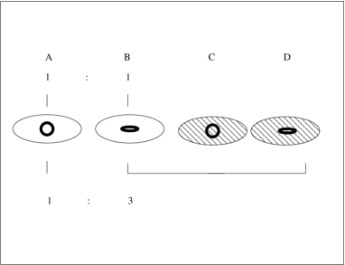
Figure 12: Schematic Representation of the three types of quasar. The empty ellipses represent a transparent host galaxy, while the filled ellipses representing dusty ones. The solid circle represents the torus around the quasar. A is hosted by a transparent galaxy, and since we are viewing the torus face on, we can see the broad line region. It is a type-1 quasar. B is also hosted by a transparent galaxy, but since the torus is edge on, we only see the narrow line region. This is a torus-obscured type-2. C has a favourable geometry, while in D the torus is in the line of sight, but since both are obscured by large scale dust in the galaxy, we cannot see the central region, so they are both host-obscured type-2s. From (Martínez-Sansigre et al., 2005) the ratio of B to A is $\sim$1:1, while the ratio of B,C and D (together) to A is $\sim$2-3:1. We note that although we are calling C and D ‘host’-obscured, the dust could plausibly be due to a nuclear starburst, with a characteristic scale $\sim 100$ pc, as well as a galaxy-scale starburst.

It is therefore not surprising that the Ly $\alpha$ (whether from the narrow-line or star-forming regions) in the host-obscured type-2s is too obscured for our exposure times (30 minutes) with a 4-m telescope: Successful spectroscopy of sub-mm galaxies in the blue requires very long integrations (1.5-6 hours) with 8-m or 10-m class telescopes (e.g. Chapman et al., 2005). We do note that AMS03 shows spatially-extended Ly $\alpha$, no other lines and no continuum, so there is a chance this object is host-obscured and the second Ly $\alpha$ line traces the starburst: this requires further study.

In Martínez-Sansigre et al. (2005), the type-2 to type-1 ratio at $z\geq 2.00$ was modelled by predicting the number of type-1 quasars which would follow the 24-$\mu$m and radio criteria. The 3.6-$\mu$m criterion was simply assumed as a way of rejecting type-1s as well as providing a rough photometric redshift. The number of $z\geq 2.00$ type-1 quasars meeting the 24-$\mu$m was predicted from the B-band luminosity function of Wolf et al. (2003), converting from B-band to 24-$\mu$m using the Rowan-Robinson (1995) SED. The optical-to-radio correlation of Cirasuolo et al. (2003) was then used to predict what fraction of the 24-$\mu$m detected type-1s would also meet the radio criterion. This modelling predicted 4.3${}^{+2.2}_{-1.1}$ such type-1 quasars, at $z\geq 2.00$ and in our 3.8 deg² field. There are 5 narrow-line objects in our sample with spectroscopically confirmed $z\geq 2.00$, and the quasar type-2 to type-1 ratio for narrow-line (torus-obscured) type-2s and type-1 quasars is therefore $\sim$1:1. For the blank objects, the crude photometric redshifts can be used to estimate, on average, how many blank (host-obscured) objects are at $z\geq 2$. There are 6 such objects, and so in (Martínez-Sansigre et al., 2005) the ratio of total number of type-2s (host- and torus-obscured) to type-1s was estimated to be 11/4 or $\sim$3:1. Since then AMS06 has been shown spectroscopically to lie at $z\leq 2.00$ the current number of objects at $z\geq 2.00$ is 10. From the errors in the modelled number of type-1 quasars, and the Poisson errors in our sample, the ratio of type-2 to type-1 quasars is found to be 2.3${}^{+1.8}_{-1.2}$. In a future paper we will calculate better photometric redshifts, to try and obtain a more reliable estimate of the quasar fraction at $z\geq 2$.

The ‘two types of type-2’ quasar, and a type-1 quasar are schematically represented in Figure 12. For a quasar to be of type-1 it has to lie in a relatively dust free galaxy (a ‘transparent’ galaxy) as well as having a favourable orientation to the torus (case A in Figure 12). A quasar in a transparent galaxy, with an unfavourable angle to the torus will not outshine its host galaxy, but the narrow-line region will still be visible (case B: a torus-obscured type-2). When the host galaxy is dusty enough to obscure the quasar (cases C and D) it is no longer possible to see the central region, whether we have a favourable angle to the torus (C) or not (D). Objects of case C and D are likely to yield blank spectra, and are indistinguishable from each other with the current dataset. Observations at radio frequencies, however, could shed some light on the orientation if radio jets are present.

This simple picture is likely to be applicable only to radio-quiet objects, since the powerful radio jets are likely to be capable of removing dust on large scales (Baker et al., 2002; Willott et al., 2002). Therefore, although the ratio of type-2 to type-1 is likely to be $\sim$2-3:1 for radio-quiet samples (and for all non-radio-selected samples, since radio-quiet objects will dominate), it should be closer to 1:1 for radio-loud samples. Thus radio-loud samples will have few ‘host-obscured’ quasars (cases C and D, although some are probably present in the sample of Willott et al., 2001) and the quasar fraction measured in these radio-loud samples will be dominated by the geometry of the torus. This picture is therefore consistent with the ratio of narrow-line to broad-line quasars predicted by unified models and found for radio-loud objects ($\sim$1:1 e.g Willott et al., 2000).

Inferring a type-2 to type-1 ratio $\sim$2-3:1 for the sample presented in this article does not disagree with the receding-torus models (e.g. Lawrence, 1991; Simpson, 2005), since the obscuring mechanism for ‘host-obscured’ type-2s is unrelated to the torus orientation or geometry. The ratio of torus-obscured (B) to type-1 (A) quasars predicted for our sample is $\sim$1:1 (and indeed consistent with the receding-torus: Figure 2 of Martínez-Sansigre et al., 2005). This phenomenon of host-obscuration might also be present in the Seyfert-2s at $z\sim 1$ that dominate the hard X-ray background, in which case care must be taken to separate the obscuring mechanism necessary to explain the AGN dominating the X-ray background from modifications to the unified schemes such as the receding torus.

The ratio of $\sim$2-3:1 found for this sample is similar to the ratio required for Seyfert-2s to Seyfert-1s at $z\sim 1$ to fit the hard X-ray background, although a ratio $\sim$2-3:1 for the quasars is not required by the hard X-ray background (Ueda et al., 2003; Treister & Urry, 2005). We do note, that due to the range in gas-to-dust ratios, some of the X-ray obscured quasars that contribute to the hard X-ray background are not necessarily type-2s in the optical sense (they might only be reddened quasars with $A_{\rm V}\sim 1-3$ but a large gas-to-dust ratio). However, at least in our sample, we find the ratio of all type-2s (B, C and D) to type-1 (A) is $\sim$2-3:1: a higher type-2 to type-1 ratio than is found in deep X-ray surveys. This suggests that indeed, 24-$\mu$m selection can find type-2 quasars that X-ray selection in the 2-10 keV band has not been able to detect, and therefore a number of the type-2 quasars presented here should be Compton-thick. This, of course, can be tested via X-ray follow-up of this or a similar sample.

References

- Alexander et al. (2003) Alexander D. M., et al., 2003, AJ, 126, 539
- Alexander et al. (2005) Alexander D. M., Chartas G., Bauer F. E., Brandt W. N., Simpson C., Vignali C., 2005, MNRAS, 357, L16
- Antonucci (1993) Antonucci R., 1993, ARA&A, 31, 473
- Baker et al. (2002) Baker J. C., Hunstead R. W., Athreya R. M., Barthel P. D., de Silva E., Lehnert M. D., Saunders R. D. E., 2002, ApJ, 568, 592
- Best et al. (2000) Best P. N., Röttgering H. J. A., Longair M. S., 2000, MNRAS, 311, 23
- Blundell & Rawlings (2001) Blundell K. M., Rawlings S., 2001, ApJL, 562, L5
- Bohlin et al. (1978) Bohlin R. C., Savage B. D., Drake J. F., 1978, ApJ, 224, 132
- Bouchet et al. (1985) Bouchet P., Lequeux J., Maurice E., Prevot L., Prevot-Burnichon M. L., 1985, A&A, 149, 330
- Brandl et al. (2004) Brandl B. R. et al., 2004, ApJS, 154, 188
- Broadhurst & Lehar (1995) Broadhurst T., Lehar J., 1995, ApJL, 450, L41+
- Bruzual & Charlot (2003) Bruzual G., Charlot S., 2003, MNRAS, 344, 1000
- Chapman et al. (2005) Chapman S. C., Blain A. W., Smail I., Ivison R. J., 2005, ApJ, 622, 772
- Chiaberge et al. (1999) Chiaberge M., Capetti A., Celotti A., 1999, A&A, 349, 77
- Cirasuolo et al. (2003) Cirasuolo M., Celotti A., Magliocchetti M., Danese L., 2003, MNRAS, 346, 447
- Cole et al. (2001) Cole S., et al., 2001, MNRAS, 326, 255
- Comastri et al. (1995) Comastri A., Setti G., Zamorani G., Hasinger G., 1995, A&A, 296, 1
- (17) Condon J. J., 1992, ARA&A, 30, 575
- Condon et al. (2003) Condon J. J., Cotton W. D., Yin Q. F., Shupe D. L., Storrie-Lombardi L. J., Helou G., Soifer B. T., Werner M. W., 2003, AJ, 125, 2411
- Croom et al. (2004) Croom S. M., Smith R. J., Boyle B. J., Shanks T., Miller L., Outram P. J., Loaring N. S., 2004, MNRAS, 349, 1397
- Czerny et al. (2004) Czerny B., Li J., Loska Z., Szczerba R., 2004, MNRAS, 348, L54
- Fadda et al. (2004) Fadda D., Jannuzi B. T., Ford A., Storrie-Lombardi L. J., 2004, AJ, 128, 1
- Fadda et al. (2006) Fadda D., et al., 2006 astro-ph/0603488
- Fanaroff & Riley (1974) Fanaroff B. L., Riley J. M., 1974, MNRAS, 167, 31P
- Gaskell et al. (2004) Gaskell C. M., Goosmann R. W., Antonucci R. R. J., Whysong D. H., 2004, ApJ, 616, 147
- Gilli et al. (2001) Gilli R., Salvati M., Hasinger G., 2001, A&A, 366, 407
- Granato & Danese (1994) Granato G. L., Danese L., 1994, MNRAS, 268, 235
- Grimes et al. (2004) Grimes J. A., Rawlings S., Willott C. J., 2004, MNRAS, 349, 503
- Hopkins et al. (2004) Hopkins et al., 2004, AJ, 128, 1112
- Jarvis et al. (2001a) Jarvis et al., 2001a, MNRAS, 326, 1563
- Jarvis et al. (2001b) Jarvis M. J., Rawlings S., Eales S., Blundell K. M., Bunker A. J., Croft S., McLure R. J., Willott C. J., 2001b, MNRAS, 326, 1585
- Jarvis et al. (2005) Jarvis M. J., van Breukelen C., Wilman R. J., 2005, MNRAS, 358, L11
- Kukula et al. (2001) Kukula M. J., Dunlop J. S., McLure R. J., Miller L., Percival W. J., Baum S. A., O’Dea C. P., 2001, MNRAS, 326, 1533
- Lacy et al. (2004) Lacy M., et al., 2004, ApJS, 154, 166
- Lacy et al. (2005a) Lacy M., Canalizo G., Rawlings S., Sajina A., Storrie-Lombardi L., Armus L., Marleau F. R., Muzzin A., 2005a, MmSAI, 76, 154
- Lacy et al. (2005) Lacy M., et al., 2005b, ApJS, 161, 41
- Lawrence (1991) Lawrence A., 1991, MNRAS, 252, 586
- Leipski et al. (2005) Leipski C., et al., 2005, A&A, 440, L5
- Lonsdale et al. (2003) Lonsdale C. J., et al., 2003, PASP, 115, 897
- Madau et al. (1994) Madau P., Ghisellini G., Fabian A. C., 1994, MNRAS, 270, L17
- Mainieri et al. (2005) Mainieri V., Rigopoulou D., Lehmann I., Scott S., Matute I., Almaini O., Tozzi P., Hasinger G., Dunlop J. S., 2005, MNRAS, 356, 1571
- Maiolino et al. (2001) Maiolino R., Marconi A., Salvati M., Risaliti G., Severgnini P., Oliva E., La Franca F., Vanzi L., 2001, A&A, 365, 28
- Marleau et al. (2004) Marleau F. R., et al., 2004, ApJS, 154, 66
- Martínez-Sansigre et al. (2005) Martínez-Sansigre A., Rawlings S., Lacy M., Fadda D., Marleau F. R., Simpson C., Willott C. J., Jarvis M. J., 2005, Nat, 436, 666
- McCarthy (1993) McCarthy P. J., 1993, ARA&A, 31, 639
- Morganti et al. (2004) Morganti R., Garrett M. A., Chapman S., Baan W., Helou G., Soifer T., 2004, A&A, 424, 371
- Norman et al. (2002) Norman C., et al., 2002, ApJ, 571, 218
- Pei (1992) Pei Y. C., 1992, ApJ, 395, 130
- Rawlings et al. (1990) Rawlings S., Eales S., Warren S., 1990, MNRAS, 243, 14P
- Rawlings & Saunders (1991) Rawlings S., Saunders R., 1991, Nat, 349, 138
- Rawlings et al. (2001) Rawlings S., Eales S., Lacy M., 2001, MNRAS, 322, 523
- Richards et al. (2002) Richards G. T., et al., 2002, AJ, 123, 2945
- Richards et al. (2003) Richards G. T., et al., 2003, AJ, 126, 1131
- Rowan-Robinson et al. (1991) Rowan-Robinson M., et al., 1991, Nat, 351, 719
- Rowan-Robinson (1995) Rowan-Robinson M., 1995, MNRAS, 272, 737
- Salpeter (1955) Salpeter E. E., 1955, ApJ, 121, 161
- Sanders & Mirabel (1996) Sanders D. B. & Mirabel, I. F., 1996, ARA&A, 34, 749
- Serjeant et al. (1998) Serjeant S., Rawlings S., Lacy M., McMahon R. G., Lawrence A., Rowan-Robinson M., Mountain M., 1998, MNRAS, 298, 321
- Simpson (1998a) Simpson C., 1998a, MNRAS, 297, L39
- Simpson (1998b) Simpson C., 1998b, ApJ, 509, 653
- Simpson (2005) Simpson C., 2005, MNRAS, 360, 565
- Simpson et al. (1999) Simpson C., Rawlings S., Lacy M., 1999, MNRAS, 306, 828
- Stern et al. (2002) Stern D., et al., 2002, ApJ, 568, 71
- Treister et al. (2004) Treister E., et al., 2004, ApJ, 616, 123
- Treister & Urry (2005) Treister E., Urry C. M., 2005, ApJ, 630, 115
- Treister et al. (2006) Treister E., et al., 2006, ApJ, 640, 603
- Ueda et al. (1999) Ueda Y., et al., 1999, ApJ, 518, 656
- Ueda et al. (2003) Ueda Y., Akiyama M., Ohta K., Miyaji T., 2003, ApJ, 598, 886
- Urrutia et al. (2005) Urrutia T., Lacy M., Gregg M. D., Becker R. H., 2005, ApJ, 627, 75
- van Ojik et al. (1997) van Ojik R., Roettgering H. J. A., Miley G. K., Hunstead R. W., 1997, A&A, 317, 358
- Villar-Martín et al. (2005) Villar-Martín M., Tadhunter C., Morganti R., Holt J., 2005, MNRAS, 359, L5
- Weedman et al. (2006) Weedman D. W., Le Floc’h E., Higdon S. J. U., Higdon J. L., Houck J. R., 2006, ApJ, 638, 613
- Werner et al. (2004) Werner M. W., et al., 2004, ApJS, 154, 1
- Wilkes et al. (2005) Wilkes B. J., Pounds K. A., Schmidt G. D., Smith P. S., Cutri R. M., Ghosh H., Nelson B., Hines D. C., 2005, ApJ, 634, 183
- Willott et al. (1998) Willott C. J., Rawlings S., Blundell K. M., Lacy M., 1998, MNRAS, 300, 625
- Willott et al. (2000) Willott C. J., Rawlings S., Blundell K. M., Lacy M., 2000, MNRAS, 316, 449
- Willott et al. (2001) Willott C. J., Rawlings S., Blundell K. M., 2001, MNRAS, 324, 1
- Willott et al. (2002) Willott C. J., Rawlings S., Archibald E. N., Dunlop J. S., 2002, MNRAS, 331, 435
- Willott et al. (2003a) Willott C. J., et al., 2003a, MNRAS, 339, 397
- Willott et al. (2003b) Willott C. J., Rawlings S., Jarvis M. J., Blundell K. M., 2003b, MNRAS, 339, 173
- Willott et al. (2004) Willott C. J., et al., 2004, ApJ, 610, 140
- Willott (2005) Willott C. J., 2005, ApJL, 627, L101
- Wilman & Fabian (1999) Wilman R. J., Fabian A. C., 1999, MNRAS, 309, 862
- Wolf et al. (2003) Wolf C., Wisotzki L., Borch A., Dye S., Kleinheinrich M., Meisenheimer K., 2003, A&A, 408, 499
- Worsley et al. (2005) Worsley M. A., et al., 2005, MNRAS, 357, 1281
- Yan et al. (2005) Yan L., et al., 2005, ApJ, 628, 604
- Zheng et al. (2004) Zheng W., et al., 2004, ApJS, 155, 73