Flux predictions of high-energy neutrinos from pulsars

Abstract

Young, rapidly rotating neutron stars could accelerate ions from their surfaces to energies of $\sim 1$ PeV. If protons reach such energies, they will produce pions (with low probability) through resonant scattering with x-rays from the stellar surface. The pions subsequently decay to produce muon neutrinos. Here we calculate the energy spectrum of muon neutrinos, and estimate the event rates at Earth. The spectrum consists of a sharp rise at $\sim 50$ TeV, corresponding to the onset of the resonance, above which the flux drops with neutrino energy as $\epsilon_{\nu}^{-2}$ up to an upper-energy cut-off that is determined by either kinematics or by the maximum energy to which protons are accelerated. We estimate event rates as high as 10-100 km^-2 yr^-1 from some candidates, a flux that would be easily detected by IceCube. Lack of detection would allow constraints on the energetics of the poorly-understood pulsar magnetosphere.

1 Introduction

Astrophysical neutrinos of high energy ($\hbox{${{}_{\displaystyle>}\atop{}^{\displaystyle\sim}}$}1$ GeV) are expected to arise in many environments in which protons are accelerated to relativistic energies. Neutrinos produced by the decay of pions created through hadronic interactions ($pp$) or photomeson production ($p\gamma$) escape from the source and travel unimpeded to Earth, and carry information directly from the acceleration site. Neutrinos may be produced by cosmic accelerators, like those in supernova remnants (Protheroe, Bednarek & Luo, 1998), active galactic nuclei (Learned & Mannheim, 2000), micro-quasars (Distefano et al., 2002) and gamma-ray bursts (Waxman & Bahcall, 1997; Dai & Lu, 2001). To detect these neutrinos, several projects are underway to develop large-scale neutrino detectors under water or ice; AMANDA-II, ANTARES and Baikal are running, while IceCube (Halzen, 2006), NEMO and NESTOR (Carr, 2003) are under construction.

Recently, we proposed that young ($t_{age}\lesssim 10^{5}\rm yr$) and rapidly-rotating neutron stars could be intense neutrino sources (Link & Burgio 2005; hereafter LB05). For stars that have a stellar magnetic moment with a component anti-parallel to the spin axis (as we expect in half of neutron stars), ions will be accelerated off of the surface; otherwise, electrons will be accelerated. If energies of $\sim$ 1 PeV per proton are attained, pions will be produced through photomeson production as the protons scatter with surface x-rays, producing a beam of $\mu$ neutrinos with energies above $\sim 50$ TeV. Detection of such neutrinos would provide an invaluable probe of the particle acceleration processes that take place in the lower magnetosphere of a neutron star. In this paper we predict the neutrino spectrum that would result from this production mechanism to aid in the interpretation of experimental results from searches for astrophysical neutrinos. We obtain improved estimates of the event rate.

In the next section, we review the acceleration model of LB05. In Section III, we calculate the neutrino spectrum that results from this model. In Section IV, we estimate the count rates that could be seen in a km²-scale experiment such as IceCube. We conclude with a discussion of the prospects for detection of high-energy neutrinos from pulsars.

2 The Model

In the neutrino production scenario of LB05, protons (within or without nuclei) are accelerated in the neutron star magnetosphere to high enough energies to undergo resonant scattering with surface x-ray photons (the $\Delta$ resonance):

$$p\gamma\rightarrow\Delta^{+}\rightarrow n\pi^{+}\rightarrow n\nu_{\mu}\mu^{+}\rightarrow n\nu_{\mu}e^{+}\nu_{e}\bar{\nu}_{\mu}.$$ (1)

The $\Delta^{+}$ is a short-lived excited state of the proton with a mass of 1232 MeV. For this process to be effective, ions must be accelerated close to the stellar surface, where the photon density is high and the process is kinematically allowed (see below, and LB05). The plasma is tied to the magnetic field, so the acceleration can occur only in the direction of the magnetic field ${\mathbf{B}}$. In a quasi-static magnetosphere with a magnetic axis that is parallel or anti-parallel to the rotation axis, the potential drop across the field lines of a star rotating at angular velocity $\Omega=2\pi/p$ (where $p$ is the period) from the magnetic pole to the last field line that opens to infinity is of magnitude (Goldreich & Julian, 1969):

$$\Delta\Phi=\frac{\Omega^{2}BR^{3}}{2c^{2}}\simeq 7\times 10^{18}B_{12}R_{6}^{3}p_{\rm ms}^{-2}\mbox{ Volts},$$ (2)

per ion of mass number $A$ and charge $Z$. Here $B=10^{12}B_{12}\rm G$ is the strength of the dipole component of the field at the magnetic poles, $R=10^{6}R_{6}$ cm is the stellar radius and $p_{\rm ms}$ is the spin period in milliseconds. Henceforth we take $R_{6}=1$ when making estimates. In equilibrium (not realized in a pulsar), a co-rotating magnetosphere would exist in the regions above the star in which magnetic field lines close; the charge density would be $\rho_{q}\simeq eZn_{0}\simeq B/pc$ (cgs), where $n_{0}$ is the Goldreich-Julian number density of ions. Deviation from corotation will lead to charge-depleted gaps somewhere above the stellar surface, through which charges will be accelerated to relativistic energies (Ruderman & Sutherland, 1975; Arons & Scharlemann, 1979). The proton energy threshold $\epsilon_{p}$ for $\Delta^{+}$ production is given by

$$\epsilon_{p}\epsilon_{\gamma}\geq(1-\cos\theta)^{-1}\ 0.3\ {\rm GeV}^{2},$$ (3)

where $\epsilon_{\gamma}$ is the photon energy and $\theta$ is the incidence angle between the proton and the photon in the lab frame. Young neutron stars typically have temperatures of $T_{\infty}\simeq 0.1\rm\ keV$, and photon energies $\epsilon_{\gamma}=2.8kT_{\infty}(1+z_{g})\sim 0.4$ keV, where $z_{g}\simeq 0.4$ is the gravitational red-shift (for $R=9$ km and $M=1.4M_{\odot}$) and $T_{\infty}$ is the surface temperature measured at infinity. For $\theta\simeq\pi/2$, corresponding to scattering of protons near the stellar surface with photons from the stellar horizon, the proton threshold energy for the $\Delta$ resonance is then $\epsilon_{p,{\rm th}}\simeq T_{\rm 0.1keV}^{-1}$ PeV, where $T_{\rm 0.1keV}\equiv(kT_{\infty}/0.1\mbox{ keV})$. Let us compare the required energy for resonance to the potential drop per proton across ${\mathbf{B}}$:

$$\frac{\epsilon_{p,{\rm th}}}{\Delta\Phi/A}\sim 10^{-4}B_{12}^{-1}p_{\rm ms}^{2}T_{\rm 0.1keV}^{-1}A.$$ (4)

Hence, for a pulsar spinning at 10 ms, a potential drop along ${\mathbf{B}}$ of only $\sim 1$% of that across ${\mathbf{B}}$ will be sufficient to bring protons or low-mass nuclei to the resonance. Optimistically assuming that the full potential $\Delta\Phi$ is available for acceleration along field lines, a necessary condition for the $\Delta$ resonance to be reached is ($A=1$)

$$B_{12}p_{\rm ms}^{-2}T_{\rm 0.1keV}\geq 3\times 10^{-4}.$$ (5)

Assuming $T_{\rm 0.1keV}=1$, typical of pulsars younger than $\sim 10^{5}$ yr, there are 10 known pulsars within a distance of 8 kpc that satisfy this condition (Manchester et al. 2005), about half of which should have positively-charged magnetic poles; these are potentially detectable sources of $\mu$ neutrinos. The best candidates are young neutron stars, which are usually rapidly spinning and hot. Equality corresponds to the full potential across field lines being present along field lines, probably an unlikely scenario, since space charge will act to quench the electric field along ${\mathbf{B}}$. For stars in which the above inequality is easily satisfied, the protons will reach energies sufficient to undergo photomeson production if the electric field along a typical open field line is much smaller than the field across the line, the more probable situation.

In the photomeson production process of eq. (1), each muon neutrino receives 5% of the energy of the proton. [We assume, for simplicity, that the pions do not undergo subsequent acceleration]. Typical proton energies required to reach resonance are $\sim T_{\rm 0.1keV}^{-1}$ PeV, so the expected $\mu$ neutrino energies will be $\epsilon_{\nu}\sim 50T_{\rm 0.1keV}^{-1}$ TeV. Moreover, since the accelerated protons are far more energetic than the radiation field with which they interact, any pions produced through the $\Delta$ resonance, and hence, any muon neutrinos, will be moving in nearly the same direction of the protons. The radio and neutrino beams should be roughly coincident, so that some radio pulsars might also be detected as neutrino sources. We see the radio beam for only a fraction $f_{b}$ of the pulse period, the duty cycle. Typically, $f_{b}\simeq 0.1-0.3$ for younger pulsars. We take the duty cycle of the neutrino beam to be $f_{b}$ (but see below). In LB05, we estimated the phase-averaged neutrino flux at Earth resulting from the acceleration of positive ions, at a distance $d$ from the source, to be

$$\phi_{\nu}\simeq cf_{b}f_{d}n_{0}\left(\frac{R}{d}\right)^{2}P_{c},$$ (6)

where $f_{d}$ is the fraction by which the space charge in the acceleration region is depleted below the corotation density $n_{0}$, and $P_{c}$ is the conversion probability. A better estimate is

$$\phi_{\nu}\simeq 2cf_{b}f_{d}(1-f_{d})n_{0}\left(\frac{R}{d}\right)^{2}P_{c},$$ (7)

The pre-factor $f_{d}(1-f_{d})$ is a more realistic interpolation between the two regimes of complete depletion ($f_{d}=0$) and no depletion ($f_{d}=1$). In the latter case, there should be no neutrino production as the field along ${\mathbf{B}}$ is entirely quenched. The factor of two arises from inclusion of the $\bar{\nu}_{\mu}$ from eq. (1). For the purposes of calculating the spectrum, we use the following differential form for the neutrino flux:

$$\frac{d\phi_{\nu}}{d\epsilon_{\nu}}=2cf_{b}f_{d}(1-f_{d})n_{0}\left(\frac{R}{d}\right)^{2}\frac{dP_{c}}{d\epsilon_{\nu}}.$$ (8)

Here we are interested in estimating upper limits on the flux; we henceforth take $f_{d}=1/2$ and $Z=A=1$.

In LB05, we estimated $P_{c}$ by assuming that the protons reach the energy required for photomeson production immediately above the stellar surface; we then evaluated $P_{c}$ at a particular height above the stellar surface. The focus of this paper is to obtain the spectrum $dP_{c}/d\epsilon_{\nu}$. We account for the fact that the proton acceleration will take place over a finite distance above the surface. We also include the finite width of the $\Delta$ resonance in the cross section.

3 Neutrino Spectrum

Let the accelerated proton have energy $\epsilon_{p}$ and the surface photons have energy $\epsilon_{\gamma}$. Define a dimensionless energy $x=\epsilon_{p}\epsilon_{\gamma}/\epsilon_{0}^{2}$, where $\epsilon_{0}^{2}\equiv 0.3$ GeV². To account for the finite width of the $\Delta$ resonance, let us express the resonant contribution to the energy-dependent $p\gamma$ cross section for a proton of energy $\epsilon$ in the nucleon rest frame as

$$\sigma=\sigma_{0}\exp\left(\frac{-(\epsilon-\epsilon_{T})^{2}}{2w^{2}}\right)\qquad\mbox{for $\epsilon>\epsilon_{T}-w$},$$ (9)

where $\sigma_{0}=5\times 10^{-28}$ cm^-2 is the cross section for $\Delta^{+}$ production, $\epsilon_{T}$ is the $\Delta$ energy threshold and $w\simeq 100$ MeV is the width of the $\Delta$ resonance. For a given photon energy and scattering angle, the proton energy at the resonance is given by

$$\epsilon_{T}=\frac{\epsilon_{0}^{2}}{\epsilon_{\gamma}}(1-\cos\theta)^{-1}\Longrightarrow x_{T}=(1-\cos\theta)^{-1}.$$ (10)

The cross-section is non-zero for $x>x_{T}-x_{w}$ where $x_{w}\equiv w\epsilon_{\gamma}/\epsilon_{0}^{2}\simeq 0.1$. This implies a minimum kinematic scattering angle $\theta_{0}$ given by

$$\cos\theta_{0}=1-(x+x_{w})^{-1}.$$ (11)

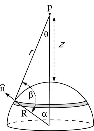
Figure 1: Geometrical setup. See text for details.

In Fig. 1 we show the geometry that we use for calculating the spectrum. We neglect the effects of gravitational light bending, which would act to increase the rates we calculate here. The proton is located at the point denoted by $p$, at a height $z$ above the stellar surface, and $\theta$ is the scattering angle between the proton and the incoming photon. The scattering angle $\theta$ is always less than $\pi/2$, which requires the protons to have energies that satisfy $x>1-x_{w}$ in order to undergo resonant scattering. There is also a maximum scattering angle $\theta_{h}$ defined by the stellar horizon as seen from height $z$:

$$\sin\theta_{h}=(1+z)^{-1},$$ (12)

where $z$ is the height above the stellar surface in units of the stellar radius $R$. We must have $\theta_{0}<\theta_{h}$ for resonance to occur. We can rewrite the cross-section as

$$\sigma(x,\theta)=\sigma_{0}\exp\left(\frac{-(x-x_{T})^{2}}{2x_{w}^{2}}\right)\qquad\mbox{for $x>x_{T}-x_{w}$}.$$ (13)

Figure 2: The neutrino energy flux is displayed for the Crab and the Vela pulsars, for the cases of linear (solid line) and quadratic proton acceleration (dashed line).

To calculate the conversion probability, we need the number density of photons as a function of height $z$ and incident photon angle $\theta$. Let the number density of photons at the stellar surface be $n_{\gamma}(0)$. An element of surface radiates into $2\pi$ steradians, independent of angle. For a small surface element of area $dA$, the contribution $dn$ to the total photon number density $n$ is

$$dn=\frac{n_{\gamma}(0)}{2\pi}\frac{dA}{r^{2}}\,\hat{n}\cdot\hat{r}\qquad\qquad\hat{n}\cdot\hat{r}=\cos(\alpha+\theta).$$ (14)

Taking the ring surface element shown in the figure, that area is

$$dA=2\pi R^{2}\sin\alpha\,d\alpha.$$ (15)

Some useful trigonometric identities are

$$r\sin\theta=R\sin\alpha\qquad(1+z)\sin\theta=\sin\beta\qquad\beta=\pi-\alpha-\theta,$$ (16)

which give

$$\alpha=\sin^{-1}[(1+z)\sin\theta]-\theta$$ (17)

$$\frac{d\alpha}{d\theta}=\frac{(1+z)\cos\theta}{\sqrt{1-(1+z)^{2}\sin^{2}\theta}}-1.$$ (18)

The derivative has a singularity at

$$\theta_{h}=\sin^{-1}\frac{1}{1+z},$$ (19)

which corresponds to the horizon angle of eq. [12]. The number density of photons at height $z$, arriving from angles in the range $\theta$ to $\theta+d\theta$ is

$$dn(z,\theta)=n_{\gamma}(0)\,d\theta\,\frac{d\alpha}{d\theta}\frac{\sin^{2}\theta}{\sin\alpha}\cos(\alpha+\theta).$$ (20)

Suppose the protons have an energy that depends on the height over which they have been accelerated: $\epsilon(z)$. At height $z$, the mean-free-path $l(x,\theta)$ for $p\rightarrow\Delta^{+}$ conversion through scattering with a photon arriving at an angle between $\theta$ and $\theta+d\theta$ is given by

$$l^{-1}(z,\theta)=dn(z,\theta)\,\sigma(\epsilon(z),\theta).$$ (21)

To obtain the total mean-free-path for conversion at height $z$, we integrate over all possible angles for the incident photons:

$$l^{-1}(z)=\int_{\theta_{0}}^{\theta_{h}}d\theta\frac{dn(z,\theta)}{d\theta}\sigma(\epsilon(z),\theta).$$ (22)

The probability for $p\rightarrow\Delta^{+}$ conversion of a proton as it moves from $z$ to $z+dz$ is

$$dP_{c}=\frac{R}{l(z)}dz.$$ (23)

Let us now assume a specific dependence of the proton energy on height:

$$x=\left(\frac{z}{L}\right)^{\gamma},$$ (24)

where $L$ is the characteristic acceleration length of the proton in units of $R$. Then

$$dz=\frac{L}{\gamma}x^{1/\gamma-1}dx.$$ (25)

The probability of conversion per unit (dimensionless) energy interval is

$$\frac{dP_{c}}{dx}=\frac{RLx^{1/\gamma-1}}{\gamma}\int_{\theta_{0}}^{\theta_{h}}d\theta\frac{dn(x,\theta)}{d\theta}\sigma(x,\theta)$$ (26)

This is the energy spectrum of converted $\Delta^{+}$ particles. The neutrino spectrum is the same, but is scaled down in energy according to $x_{\nu}=0.05x$. The amplitude increases by a factor of 20 to maintain total probability. From eq. (8) we find (in units of GeV^-1 m^-2 s^-1)

$$\frac{d\phi_{\nu}}{d\epsilon_{\nu}}=1.1\times 10^{-3}f_{b}B_{12}p_{\rm ms}^{-1}d_{\rm kpc}^{-2}\frac{dP_{c}}{d\epsilon_{\nu}}$$ (27)

where $n_{0}=7\times 10^{13}B_{12}p_{\rm ms}^{-1}$ $\rm cm^{-3}$. We obtain $dP_{c}/d\epsilon_{\nu}$ from eq. (26). Since $x_{\nu}=0.05x$, we have

$$\frac{dP_{c}}{d\epsilon_{\nu}}=20\frac{\epsilon_{\gamma}}{\epsilon_{0}^{2}}\frac{dP_{c}}{dx}=2.7\times 10^{-5}\,T_{\rm 0.1keV}\frac{dP_{c}}{dx}\,\,\mbox{GeV${}^{-1}$}.$$ (28)

Combining eq. (28) with eq. (8) gives the neutrino energy flux:

$$\frac{d\phi_{\nu}}{d\epsilon_{\nu}}=3\times 10^{-8}f_{b}B_{12}p_{\rm ms}^{-1}d_{\rm kpc}^{-2}T_{\rm 0.1keV}\frac{dP_{c}}{dx}$$ (29)

Eq. (29) is our chief result. It allows comparison with observed event distributions as well as an estimate of the total expected counts. In Fig. 2 we show the neutrino energy flux for two candidate sources, the Crab and Vela pulsars, located respectively in the northern and southern hemispheres. For illustration, we consider linear ($\gamma=1$) and a quadratic ($\gamma=2$) proton acceleration laws. Linear acceleration corresponds to an accelerating field that is constant in space. Quadratic acceleration corresponds to an accelerating field that grows linearly with height above the star. We have used $x_{w}=0.1$.

For either acceleration law, the spectrum begins sharply at

$$\epsilon_{\nu}\simeq 70T_{\rm 0.1keV}^{-1}\mbox{ TeV},$$ (30)

corresponding to the onset of the resonance. At higher energies, the spectrum drops approximately as $\epsilon_{\nu}^{-2}$, as the phase space for conversion becomes restricted; higher energy neutrinos are produced by protons that have been accelerated to greater heights, where the photon density is lower and the solid angle subtended by the star (as seen by the proton) is smaller. At some maximum energy, the spectrum is suddenly truncated by either kinematics (solid curve) or the termination of the proton acceleration as limited by the magnitude of the acceleration gap (not shown, since this cut-off has not been predicted).

In obtaining eq. (29), we neglected the effects of general relativity, except when relating the stellar temperature at infinity to the temperature near the surface. General relativistic effects bend the photon trajectories and bring some photons from beyond the classical stellar horizon (eq. 12) to where they can interact with the protons. This effect enhances the rate, but not significantly. To estimate the magnitude of this effect, we can regard the star as effectively larger, and replace the stellar radius that appears as a pre-factor in eq. (26) by the effective stellar radius at infinity, $(1+z_{g})R$. The effects of gravitational light bending will increase the flux by a factor of $\simeq 1+z_{g}\simeq 1.4$ for $R=9$ km and a factor of only $1.2$ for $R=12$ km. In light of the large uncertainties in the values of $f_{d}$ and $L$, we simply took $R=10$ km in eq. (26) for the purpose of making estimates.

Source	$d_{\rm kpc}$	age	$p_{\rm ms}$	$B_{12}$	$T_{\rm 0.1keV}$	$f_{b}$	$P_{c}$	$dN/dAdt$
		yr						km-2 yr-1
Crab	2	$10^{3}$	33	3.8	$\leq 1.7$ (Weisskopf et al., 2004)	0.14	$\rm 1.6\times 10^{-3}$	45
Vela	0.29	$10^{4.2}$	89	3.4	0.6 (Pavlov et al., 2001)	0.04	$\rm 7.2\times 10^{-5}$	25
J0205+64	3.2	$10^{2.9}$	65	3.8	$\leq 0.9$ (Slane et al., 2002)	0.05	$\rm 2.4\times 10^{-4}$	1
B1509-58	4.4	$10^{3.2}$	151	15	1?	0.26	$\rm 3.4\times 10^{-4}$	5
B1706-44	1.8	$10^{4.3}$	102	3.1	1?	0.13	$\rm 3.4\times 10^{-4}$	5
B1823-13	4.1	$10^{4.3}$	101	2.8	1?	0.34	$\rm 3.4\times 10^{-4}$	2
Cass A	3.5	300	10?	1?	4 (Pavlov et al., 2004)	0.1?	$2.1\times 10^{-2}$	50
SN 1987a	50	17	1?	1?	4?	0.1?	$2.1\times 10^{-2}$	3

Table 1: Estimated upper limits on the $\mu$ fluxes at Earth. Numbers followed by question marks indicate guesses. Radio pulsar spin parameters were taken from the catalogue of the Parkes Radiopulsar Survey (Manchester et al. 2005). Temperatures and limits on temperatures were taken from the references indicated. The temperature upper limits on the Crab and J0205+64 were used. The integrated conversion probability $P_{c}$ is reported for the case of linear acceleration, and assuming $L=0.1$.

4 Estimated Count Rates

We now use the spectrum obtained in the previous section to estimate the count rate in a detector. Large-area neutrino detectors use the Earth as a medium for conversion of a muon neutrino to a muon, which then produces Čerenkov light in the detector. The conversion probability in the Earth is (Gaisser et al. 1995):

$$P_{\nu_{\mu}\rightarrow\mu}\simeq 1.3\times 10^{-6}\left(\frac{\epsilon_{\nu}}{\mbox{1 TeV}}\right)$$ (31)

The muon event rate is

$$\frac{dN}{dAdt}=\int_{\epsilon_{T}}^{10\epsilon_{T}}d\epsilon_{\nu}\frac{d\phi_{\nu}}{d\epsilon_{\nu}}P_{\nu_{\mu}\rightarrow\mu}.$$ (32)

The choice of the upper limit of integration is not very important, because the spectrum is steep. Estimated count rates are given in the last column of Table 1 for the Crab, Vela and 9 other pulsars, assuming $L=0.1$ and linear acceleration. Estimated conversion probabilities for $p\rightarrow\Delta^{+}$, obtained by integrating eq. (26) from $x_{T}$ to $10x_{T}$, are shown in the penultimate column. Our event rates are a factor of $\sim 10-30$ lower than estimated in LB05. The main reason for the lowered rate is phase space limitations imposed by the geometry; protons at a given height can only undergo resonant conversion from photons arriving from the surface in a narrow range of angles. Moreover, there is a competition between the finite distance over which protons reach sufficient energy to be converted, and the reduction in the number of photons arriving from the star with the correct angular range for resonant conversion to be kinematically allowed.

Figure 3: The muon event rate is shown as a function of the acceleration length for the Crab (circles) and the Vela (squares) pulsars. Upper (lower) curves display results for the case of linear (quadratic) proton acceleration. Solid and dashed lines guide the eye.

In Fig. 3 we show the muon event rates estimated for the Crab (circles) and the Vela pulsars (squares), as a function of the acceleration length $L$. The upper curves refer to calculations performed for a linear acceleration law, whereas the lower ones assume a quadratic one. The event rate increases up to a maximum value, and then decreases. Increasing $L$ initially enhances the rate because the protons then attain enough energy to undergo resonant scattering at a height where much of the stellar surface is visible. If $L$ is made too large, however, the process is reduced by a lower photon density and restricted range in photon angles available for scattering. The dependence on $L$ is more gradual for the quadratic acceleration model, because the protons must travel farther to attain enough energy for resonance.

5 Discussion

To summarize, if protons reach the photomeson production resonance in the neutron star magnetosphere, they will produce a spectrum of muon neutrinos with the following simple characteristics:

1. A sharp turn on at

   $$\epsilon_{\nu}\simeq 70T_{\rm 0.1keV}^{-1}\mbox{ TeV},$$ (33)

   corresponding to the onset of the resonance.

2. A rapid fall with energy as $\epsilon_{\nu}^{-2}$, determined by scattering kinematics.

Neutrinos are produced at relatively high rates only if the protons are accelerated through the resonance close to the star ($L\hbox{${{}_{\displaystyle<}\atop{}^{\displaystyle\sim}}$}1$; see Fig. 3). We obtain integrated count rates of several to $\sim 100$ km^-2 yr^-1 for a depletion factor $f_{d}\simeq 1/2$. Such count rates should be easily detected by IceCube, and possibly by AMANDA-II or ANTARES with integration times of about a decade (IceCube is planned to have replaced AMANDA-II by then). While the characteristics of the spectrum presented here are robust, we caution that the event rates we obtain are very rough upper limits, subject to many uncertainties. For example, we have assumed that the neutrinos are beamed into the same solid angle as the radio beam, which might not be a correct assumption. The radio beam is thought to be produced within $\sim 10R$ (see, e.g., Cordes 1978). In our model, the pions are produced much closer to the star. They then propagate to $\sim 1000R$ before decaying to neutrinos. At this distance from the star, the field is not dipolar, and it is difficult to say anything definite about the distribution of pion trajectories in this region. If the neutrinos form a beam, it may be more or less collimated than the radio beam. If the neutrino beam is more collimated, the neutrino event rates would be higher than estimated here.

The first 807 d of data from AMANDA-II revealed no statistically significant sources (Groß, 2005). Intriguingly, there were 10 events (over a background of 5.4) recorded from the direction of the Crab pulsar; IceCube will be able to confirm or refute this result. While it would be more exciting to actually see neutrinos from pulsars, the accumulation of null results over the next decade would be interesting as well; it would probably mean that photomeson production is ineffective or non-existent in the neutron star magnetosphere, thus providing a bound on the accelerating potential.

References

- Arons & Scharlemann (1979) Arons J., Scharlemann E. T., 1979, ApJ, 231, 854
- Carr (2003) Carr J., 2003, Nucl. Phys. (Proc. Suppl.) 118, 383
- Cordes (1978) Cordes, J. M., 1978, ApJ, 222, 1006
- Dai & Lu (2001) Dai Z. G., Lu T., 2001, ApJ, 551, 249
- Distefano et al. (2002) Distefano C., Guetta D., Waxman E., Levinson A., 2002, ApJ, 575, 378
- Gaisser et al. (1995) Gaisser, T. K., Halzen, F., Stanev, T., 1995, Phys. Rep. 258, 173, Erratum ibid. 271, 355
- Goldreich & Julian (1969) Goldreich P., Julian W. H., 1969, ApJ 395, 250
- Groß (2005) Groß, A. for the AMANDA Collaboration, Proceedings of the 40th Rencontres de Moriond on Electroweak Interactions and Unified Theories, La Thuile, Italy, 5-12 March, 2005; e-print: astro-ph/0505278
- Halzen (2006) Halzen F., 2006, Eur. Phys. J., C46, 669
- Learned & Mannheim (2000) Learned, J.G., Mannheim, K., 2000, Ann. Rev. Nucl. Part. Sci. 50, 679
- Link & Burgio (2005) Link B., Burgio G. F., 2005, Phys. Rev. Lett., 94, 181101
-
Manchester et al. (2005)
Manchester, R.N., Hobbs, G.B., Teoh, A., Hobbs, M., 2005, AJ, 129, 1993;
www.atnf.csiro.au/research/pulsar/psrcat/ - Pavlov et al. (2001) Pavlov G. G., Zavlin V. E., Sanwal D., Burwitz V., Garmire G. P., 2001, ApJ 552, L129
- Pavlov et al. (2001) Pavlov G. G., Sanwal D., Teter M. A., in Young Neutron Stars and Their Environments, edited by F. Camilo and G.M. Gaensler, IAU Simp. No. 218 (Astronomical Society of the Pacific, San Francisco, CA, 2004), p.239
- Protheroe, Bednarek & Luo (1998) Protheroe R. J., Bednarek W., Luo Q., 1998, AP, 9, 1
- Ruderman & Sutherland (1975) Ruderman M. A., Sutherland P. G., 1975, ApJ, 196, 51
- Slane et al. (1975) Slane P. O., Helfland D. J., Murray S. S., 2002, ApJ, 571, L145
- Waxman & Bahcall (1997) Waxman E., Bahcall J. N., 1997, Phys. Rev. Lett. , 78, 2292
- Weisskopf et al. (2004) Weisskopf M. C., O’Dell S. L., Paerels F., Elsner R. F., Becker W., Tennant A. F., Swartz D. A., 2004, ApJ 601, 1050