Strange magnification pattern in the large separation lens SDSS J1004+4112 from optical to X-rays

We present simultaneous XMM-Newton UV and X-ray observations of the quadruply lensed quasar SDSS J1004+4112 (RBS 825). Simultaneously with the XMM-Newton observations we also performed integral field spectroscopy on the two closest lens images A and B using the Calar Alto PMAS spectrograph. In X-rays the widely spaced components C and D are clearly resolved, while the closer pair of images A and B is marginally resolved in the XMM-EPIC images. The integrated X-ray flux of the system has decreased by a factor of 6 since it was observed in the ROSAT All Sky Survey in 1990, while the X-ray spectrum became much harder with the power law index evolving from $\Gamma=-2.3$ to $\Gamma=-1.86$. By deblending the X-ray images of the lensed QSO we find that the X-ray flux ratios between the lens images A and B are significantly different from the simultaneously obtained UV ratios and previously measured optical flux ratios. Our optical spectrum of lens image A shows an enhancement in the blue emission line wings, which has been observed in previous epochs as a transient feature. We propose a scenario where intrinsic UV and X-ray variability gives rise to line variations which are selectively magnified in image A by microlensing. The extended emission of the lensing cluster of galaxies is clearly detected in the EPIC  images, we measure a 0.5-2.0 keV luminosity of $1.4\times 10^{44}{\rm erg/s}$. Based on the cluster X-ray properties, we estimate a mass of $2-6\times 10^{14}{\rm M_{\odot}}$.

1 Introduction

The lensed QSO SDSS J1004+4112 was originally found as an X-ray source in the ROSAT All Sky Survey (RASS) and entered the ROSAT Bright Source catalogue under the designation RBS 825 (Schwope et al., 2000). The brightest optical counterpart within the RASS error circle turned out to be a type I QSO at z=1.73 and was regarded as the unique identification of the unresolved X-ray source.

Its lensed nature was discovered in a survey of large separation lenses using the Sloan Digital Sky Survey (SDSS) (Inada et al., 2003). Optical imaging revealed 4 images of the quasar, with a maximum separation of $14.6^{\prime\prime}$ it is the largest separation lensed QSO known so far. A faint 5th image was detected in deep HST imaging by Inada et al. (2005). The lensing object is a cluster of galaxies at z=0.68, the quasar itself has a redshift of z=1.73. SDSS J1004+4112 is the first multiple quasar where the lensing gravitational potential is dominated by a cluster of galaxies, and not a single galaxy. Modelling of the lensing potential gives only a rough estimate of the cluster mass ($M\geq 10^{14}h^{-1}M_{\odot}$, Oguri et al. 2004). Similarly the predictions for the time delays between the images are uncertain, the delay between the closest components A and B can be up to $37\,h^{-1}$ days, the largest delay C-D could be up to $3000\,h^{-1}$ days. Most models of the lens predict a delay sequence C–B–A–D of the images, but the ordering D–A–B–C is also possible (Oguri et al., 2004). Optical spectroscopy of the individual components revealed significant differences in the emission line profiles of the components: the blue wings of the emission lines were found to be enhanced in the spectra of component A (Richards et al., 2004) at certain epochs in 2003. This was interpreted as an indication for the presence of microlensing in lens image A. In this paper we present simultaneous multi-waveband observations of SDSS J1004+4112 from optical spectroscopy to UV and X-ray observations with XMM-Newton . In Section 2 we describe the analysis of the XMM-Newton data, the results are compared with an earlier epoch ROSAT observation in Section 3. In Section 6 we attempt an explanation of the unusual spectral energy distributions of the lens images (see Section 4) and the equally puzzling differences in the emission line profiles between the QSO images A and B (see Section 5).

If not stated otherwise, all statistical error values given throughout the paper are $1\sigma$ limits. All luminosities were calculated using the cosmological parameters $H_{0}=70\;{\rm km\;s^{-1}Mpc^{-1}}$, $\Omega_{\rm M}=0.27$, and $\Omega_{\Lambda}=0.73$

2 XMM Newton observations

SDSS J1004+4112  was observed by XMM-Newton on 20/04/2004 under observation ID 0207130201 for a total of 60 ksec. The primary instruments were the 3 EPIC (European Photon Imaging Camera) imaging CCDs, observing simultaneously with the optical monitor (OM) and the RGS grating spectrometers. A summary of the EPIC and OM observations is given in Table 1. The RGS spectra do not show sufficient signal for scientific analysis and are not discussed here.

Table 1: Summary of XMM-Newton observations

Instr.	Filter	Date	Start UT	exp. [s]
EMOS1	Thin1	2004-04-20	02:59:04	60473
EMOS2	Thin1	2004-04-20	02:59:03	60478
EPN	Thin1	2004-04-20	03:21:24	58836
OM	U	2004-04-20	03:03:00	8000
OM	UVW1	2004-04-20	04:58:08	9370
OM	UVM2	2004-04-20	04:58:08	15364

2.1 X-ray data analysis

The data were processed from observation data files (ODFs) using the XMM Science Analysis Software (SAS) version 6.5. Part of the EPIC exposure time was affected by high particle background. Since the background contamination is not severe and SDSS J1004+4112  is a relatively bright X-ray source, we decided not to screen out the times of enhanced background but to use all available data. The images were binned with 2 arcseconds per pixel in order to optimally sample the 5 arcsec (FWHM) PSF of the XMM telescopes. For each of the 3 EPIC cameras we created 5 images in the energy bands listed in table 2.

Table 2: EPIC image energy bands

band 1	0.2-0.5 keV
band 2	0.5-1.0 keV
band 3	1.0-2.0 keV
band 4	2.0-4.5 keV
band 5	4.5-12.0 keV

The corresponding exposure maps for each image and detection masks were calculated using the XMM-SAS  tasks eexpmap and emask. The background maps were constructed using the SAS task esplinemap by fitting a spatially flat component plus a component following the vignetting function of the X-rays telescopes to source-free regions of the EPIC images.

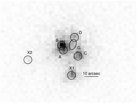
Figure 1: Combined EPIC MOS image (0.2-4.5 keV) of SDSS J1004+4112  with positions of sources used in PSF fitting.

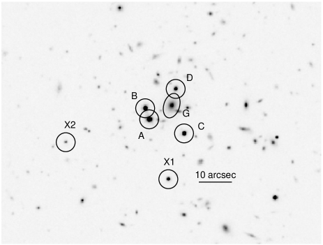
Figure 2: Archival subaru I-band image of SDSS J1004+4112  with source positions as in Fig. 1.

2.1.1 PSF fitting and extended emission from the lensing cluster

To measure the X-ray flux of each of the partly confused lens components and to search for the presence of diffuse X-ray emission from the lensing cluster, we performed multi-PSF fitting on the XMM EPIC X-ray images.

The physical pixel size of the 2 EPIC MOS cameras is 40 $\times$ 40 ${\rm\mu m}$, corresponding to 1.1 arcsec. The EPIC PN pixel size of 150 $\times$ 150 ${\rm\mu m}$ corresponds to 4.1 arcseconds, undersampling the PSF of the X-ray telescope. Since the angular distance between the closest components of SDSS J1004+4112  is 3.8 arcsec, slightly smaller than the FWHM of the XMM XRTs, only the well sampled images of the EPIC MOS cameras are used for the PSF fitting described here.

We have used the XMM SAS task emldetect to perform multi-PSF fitting on EPIC MOS images. The version of emldetect from SAS release 6.5 was modified to use the “extended accuracy” calibration PSF. The “medium accuracy” PSF model, which is normally used by emldetect is the only calibration PSF model, which includes the azimuthal asymmetries of the XMM PSF at large off-axis angles. However, near the optical axis, the “extended accuracy” PSF is a more accurate representation of the radial brightness profile. Any spatial variations of the exposure maps and the background maps are incorporated in the fitting model.

Apart from the four lensed components of SDSS J1004+4112 , another two X-ray point sources are visible in the immediate vicinity of SDSS J1004+4112 . These sources, labelled with X1 and X2 in Fig. 1, can also be identified with optical counterparts in Subaru images (see Fig. 2) and are presumably unrelated AGN. Object X1 has been used to tie the astrometry of the XMM image to the astrometric frame of the Subaru images.

The optical positions of the 4 lens components, and the objects X1 and X2, were then used as fixed input positions for multi-PSF fitting of point-like sources. The fits were performed on a co-added MOS1+MOS2 broad band image in the energy range 0.2-4.5 keV as well as on a set of 5 images in the bands described in Table 2.

After the subtraction of the 6 point sources with their best fit fluxes it became obvious that extended emission from the lensing cluster of galaxies is present in the X-ray images. Therefore we added an extended component (the instrumental PSF convolved with a King profile) to the fitting procedure. The core radius and the position of the extended source was left free to vary. This model was fitted to the broad band EPIC MOS image.

The best fit position of the extended source is $\alpha$=10h04m33.9, $\delta$=41d12m50.6s, close to quasar image D. The resulting core radius is $r_{c}=30^{\prime\prime}$. We used these values as fixed input parameters to obtain fluxes for the cluster and the point sources in each of the 5 X-ray energy bands. The results are summarized in table 3. The point source fluxes resulting from these fits are also used in the discussion of the X-ray properties of the lens images and are the basis of the spectral energy distributions shown in Figs. 6 & 7

We measure a 0.5-2.0 keV luminosity of $1.4\times 10^{44}{\rm erg\;s^{-1}}$. Fig.3 shows that the extended cluster emission is asymmetric with respect to the brightest cluster galaxy and the lensing centre.

From the count rates in the 5 standard EPIC MOS energy bands we constructed a 5-point spectrum which we fitted with a mekal model at the cluster redshift of z=0.68 and a fixed metallicity of $Z=0.5$, which was measured for clusters of this redshift range (Tozzi et al., 2003). We derived a best fit gas temperature of $T=4.3^{+2.1}_{-1.0}{\rm keV}$. With the scaling relations for clusters at this redshift (Kotov & Vikhlinin, 2005) its luminosity and temperature puts the cluster in the mass range $2-6\times 10^{14}{\rm M_{\odot}}$, consistent with, and improving the estimates from lensing models.

The best fit centroid of the cluster extended emission is located 7 arcseconds northwest of the brightest cluster galaxy. The offset well exceeds the statistical $1\sigma$ positional error (0.4 arcsec) of the extended X-ray source. However, the Chandra image of SDSS J1004+4112 (Ota et al., 2006) shows a peak of the diffuse X-ray emission at the position of the BCG. The discrepancy can be understood, since due to dominance of the QSO point sources at the centre of the cluster, the fit to the EPIC MOS image will be dominated by the outer regions of the cluster emission. Indeed, Fig. 2 shows, that the outer contours of the X-ray emission are offset from the BCG to the northwest. This may be an indication that the cluster is not in a fully relaxed state.

Table 3: Fluxes

band	flux of component
	A	B	C	D	cluster
keV	$10^{-15}{\rm erg/(cm^{2}s)}$
0.2-0.5	$6.7\pm 1.2$	$21.7\pm 1.3$	$11.8\pm 1.0$	$4.8\pm 0.8$	$17.8\pm 3.3$
0.5-1.0	$19.3\pm 1.8$	$29.5\pm 1.8$	$20.9\pm 1.4$	$12.2\pm 1.2$	$31.1\pm 4.8$
1.0-2.0	$21.1\pm 2.0$	$38.1\pm 2.0$	$25.6\pm 1.6$	$13.7\pm 1.4$	$62.1\pm 5.9$
2.0-4.5	$17.9\pm 3.7$	$63.6\pm 3.9$	$40.0\pm 3.2$	$24.3\pm 2.8$	$46.8\pm 12.0$
4.5-12.0	$31.2\pm 6.3$	$33.1\pm 6.2$	$60.5\pm 6.4$	$21.9\pm 4.6$	$22.7\pm 24.8$

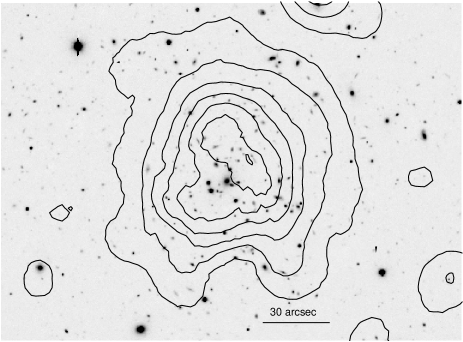
Figure 3: Subaru I band image with X-ray contours from the combined MOS images. The point sources were subtracted with fluxes as listed in table 3.

2.1.2 XMM Optical monitor data

The XMM Optical Monitor (OM) is a 30 cm telescope equipped with photon counting micro-channel plate intensified CCDs (MICs). In imaging mode various filters covering passbands from 180 nm to 600 nm can be used. The FWHM of the OM PSF ranges from 1.4 arcsec to 2.0 arcsec, depending on the filter. Due to the nature of the detectors, the measured event rates have to be corrected for the effects of dead time, coincidence losses (in case of bright sources), and a slow degradation of the detector sensitivity over the time of the mission.

We have images of SDSS J1004+4112  using the OM filters U, UVW1, UVM2 with central wavelengths 344 nm, 291 nm, and 231 nm (see Fig. 4 for the OM U-band image). The data were processed with the OM reduction pipeline omichain from SAS version 6.5. Since in the OM images the PSFs of the lens components overlap, we used PSF fitting to measure the fluxes of the components. For this purpose the backgrounds of the OM images, including the OM-typical reflection features were modelled by fitting low-order bivariate polynominal surfaces. On the background subtracted images we fitted the lens components and the close-by source ’X1’ using the GALFIT package (Peng, Impey & Rix, 2002). None of the cluster galaxies was detected in the OM images. We used a Gaussian-shaped PSF with freely variable width, forced to an identical value for all sources. This method does not necessarily produce exact values for the absolute fluxes, if the true PSF deviates significantly from the Gaussian model. However, the relative fluxes of the components, which are more important in this context, will be measured with high accuracy.

The resulting count rates were corrected for detector dead time and for the time-dependent degradation factor, as computed by the SAS task ommag. For sources in the brightness range of SDSS J1004+4112  the count rate dependent coincidence loss correction is of the order of 1% and has been neglected here. Table 4 shows a summary of the OM results.

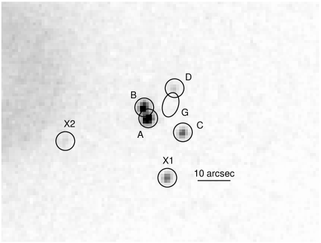
Figure 4: XMM OM U-band image of SDSS J1004+4112  with source positions as in Fig. 1.

Table 4: OM UV data

QSO image	raw rate			flux density
	[cts/sec]			$\rm{10^{-16}erg/(cm^{2}s\,\AA)}$
	U	UVW1	UVM2	(344 nm)	(291 nm)	(231 nm)
A	1.109	0.441	0.078	2.24	2.24	1.87
B	0.782	0.305	0.050	1.58	1.55	1.20
C	0.348	0.117	0.018	0.702	0.60	0.43
D	0.111	0.048	0.005	0.224	0.25	0.13

2.1.3 X-ray spectra

The lens images A and B are too close to extract individual EPIC spectra of these components. Therefore for each EPIC camera we extracted individual spectra for the components C and D as well as for the source blends A+B and for the entire complex of the 4 QSO images. We used source extraction radii of 4 arcseconds for the single components and 8 arcseconds for the A+B blend. The extraction region for the entire complex with 16 arcseconds radius encloses all 4 lens images and the core of the lensing cluster, but not the unrelated X-ray source ’X1’.

The background was extracted from source-free regions. Detector response matrices and effective areas were computed using the software and calibration files from XMM-SAS version 6.5. Spectral fits have been performed with XSPEC v22.1. For all spectral fits we used a single power law model with photoelectric absorption and an optional Fe K_α fluorescence line at 6.4 keV (AGN source frame).

The global spectrum including all lens images is fitted well by the single power law model with photon index $\Gamma=-1.86\pm 0.02$ and photon flux density $F_{\rm 1keV}=(6.50\pm 0.18)\times 10^{-5}$  cm^-2 s^-1 keV^-1 . With a best fit absorbing column density $N_{\rm H}=(1.04\pm 0.19)\times 10^{20}{\rm cm}^{-2}$ there is no indication for intrinsic or other line-of-sight absorption in excess of the galactic column density $N_{\rm H,gal}=1.14\times 10^{20}{\rm cm}^{-2}$ (Dickey & Lockman, 1990). Fig. 5 shows the EPIC spectra with the best fit power law model. The inclusion of a 6.4 keV iron fluorescence line at the redshift of the QSO does not improve the $\chi^{2}$ significantly, the best fit results in an unresolved line with equivalent width $55\pm 39$ eV at the source rest frame energy $6.48\pm 0.06$ keV.

The results of the spectral fits for the individual lens images are summarized in Table 5. None of the spectra show evidence for excess absorption. When we include a narrow Fe emission line at the source frame energy 6.4 keV, the detection is marginal for images A+B, only upper limits can be given for the line equivalent width in images C and D.

Table 5: XMM spectra of individual components:

	free $N_{\rm H}$		gal.$N_{\rm H}$	Fe$K_{\alpha}$
Image	$N_{\rm H}$	$\Gamma$	$\Gamma$	EQW
	$[10^{20}{\rm cm^{-2}}]$			[eV]
A+B	$0.55\pm.26$	$1.87\pm.03$	$1.92\pm.02$	$97\pm 59$
C	$0.53\pm.54$	$1.78\pm.05$	$1.83\pm.03$	$<82(90\%)$
D	$0.17\pm.84$	$1.69\pm.07$	$1.75\pm.04$	$<162(90\%)$

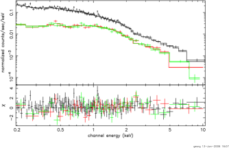
Figure 5: EPIC XMM MOS and PN spectra fitted with a single power law model. At the rest frame energy 2.3 keV a weak signature of the Fe K_α line is visible. The upper spectrum (black) is the PN spectrum with the measured data points and a line indicating the best fit model. The lower spectra (red and green) show the MOS1 and MOS2 data with the same model. See the online edition of the journal for a colour version of this figure.

2.1.4 Chandra spectra

During the refereeing process of this article, results of a Chandra observation of SDSS J1004+4112 were published as a yet unrefereed preprint (Ota et al., 2006). The Chandra observation was performed in January 2005, some 9 month after our XMM-Newton observation. We give a brief comparison of the Chandra and XMM-Newton results in Sect. 6. However, Ota et al. do not give the power law spectral indices of the individual QSO images. Therefore we extracted spectra of each QSO component from the archival Chandra data using CIAO version 3.3 and CALDB version 3.2.1. For each component we applied a source extraction radius of 1.75 arcseconds and chose a source free backround region. These spectra were fitted with single power law spectra with fixed galactic absorption. The resulting spectral indices (Table 6) can directly be compared with the corresponding values measured by XMM-Newton (Table 5). For all QSO images, the spectral indices measured by XMM-Newton and Chandra are consistent with each other. During both observations, image D exhibited a harder spectrum than the other components.

Table 6: Chandra spectral indices of individual components:

Image	$\Gamma$
A	$-1.87\pm 0.06$
B	$-1.93\pm 0.05$
C	$-1.92\pm 0.07$
D	$-1.67\pm 0.07$

For all QSO images Ota et al. (2006) give Fe $K_{\alpha}$ equivalent widths that are much larger than the corresponding values or upper limits from the (higher SNR) EPIC spectra (Table 5). Since there is considerable uncertainty about the Chandra effective area calibration at energies around 2.3 keV, where the redshifted line is measured, we do not regard this discrepancy as evidence for any spectral variability.

2.1.5 X-ray light curves

For all EPIC cameras we also extracted the events detected from the complex of images A and B with an extraction radius of 6.5 arcseconds and created background subtracted light curves with 1000 seconds bin size. The light curves do not show any indication for variability within the 16 hours interval of the observation.

3 ROSAT X-ray observations

The region of SDSS J1004+4112  was scanned between Oct 17 and Nov 9, 1990, with the ROSAT X-ray satellite during its all-sky survey (RASS). It received a total exposure of 474 seconds; 112 source photons were detected from the region of SDSS J1004+4112 . The maximum likelihood fit applied to the RASS-data was slightly indicative of a small extent (Gaussian $\sigma$ of 9″ in excess of the RASS-PSF of about 20″) of the source, however with a very low extent likelihood. There are no further observations of this region of the sky with ROSAT.

The ROSAT X-ray hardness ratios HR1$=-0.32\pm 0.09$ and HR2$=0.15\pm 0.16$ lie well in the range which are typically populated by AGNs of different flavours. The hardness ratios are defined as HR$=\frac{H-S}{H+S}$, with $H$ and $S$ being the counts in soft and hard energy channels, respectively. For HR1 and HR2 the relevant soft channels are $0.1-0.4$ and $0.5-0.9$ keV, respectively, and the relevant hard channels are $0.5-2.0$ keV and $0.9-2.0$ keV. For a more detailed spectral analysis we extracted source photons from the X-ray event lists using the MIDAS/EXSAS software. A background-corrected source spectrum was binned into 5 independent energy bins with a minimum signal-to-noise ratio of 5 per bin. The spectrum could be successfully fitted with a simple power law absorbed by cold interstellar matter with the column density fixed at the galactic value, $N_{\rm H}=1.14\times 10^{20}$ cm^-2. The best fit with reduced $\chi_{\nu}^{2}=0.2$ for 3 degrees of freedom was achieved with a power-law index $\Gamma=-2.3\pm 0.3$ and a photon flux density at $E_{0}=1$ keV of $F_{\rm E_{0}}=(4.0\pm 0.8)\times 10^{-4}$  cm^-2 s^-1 keV^-1.

Compared to the spectrum taken by XMM-Newton  14 years later, the RASS X-ray spectrum of SDSS J1004+4112  is much brighter and softer (see Fig. 6). X-ray variability between bright-soft and low-hard states has been observed in other type I AGN with a similar range of spectral slopes (e.g. NGC~4051, Lamer et al. 2003).

4 Spectral energy distribution of the lens images

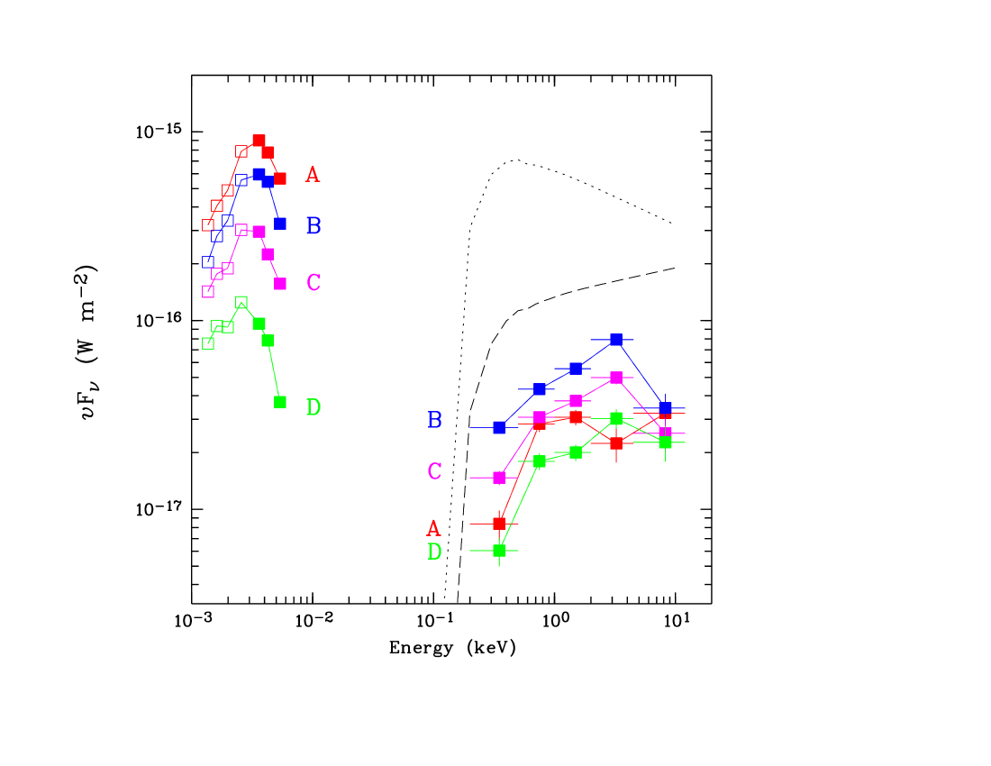
Figure 6: Spectral energy distributions (SEDs) of the lensed components of SDSS J1004+4112  from the optical to the X-ray wavelength regime in $\nu F_{\nu}$. The simultaneous XMM-Newton measurements are marked with filled squares, the earlier epoch Subaru data points are indicated by open diamonds. The lines represent the best-fit power laws for the integrated light of the lens and the QSO based on ROSAT all-sky survey (dotted) and XMM-Newton (dashed) observations. See the online edition of the journal for a colour version of this figure.

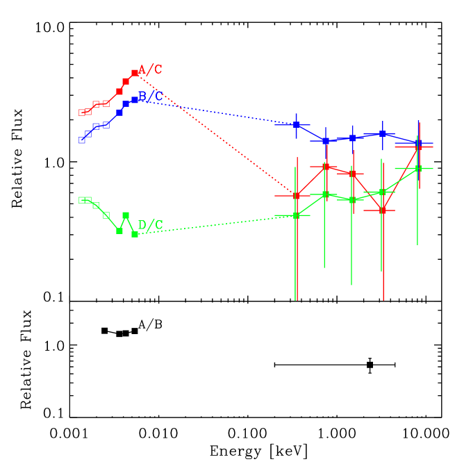
Figure 7: Top panel: SEDs of QSO components A,B, and D from the optical to the X-ray regime as in Fig. 6, but relative to component C. Bottom panel: SED of component A relative to component B. Here only simultaneous data are used: the continuum flux ratio from the optical spectrum, the XMM OM UV data, and the XMM EPIC X-ray data. See the online edition of the journal for a colour version of this figure.

With the results of the PSF fitting to the EPIC MOS images together with the results from the simultaneous XMM OM imaging and the earlier-epoch Subaru photometry (Oguri et al., 2004) we constructed spectral energy distributions (SEDs) for each lens image. Figure 6 shows a comparison of the SEDs together with integral spectra of the whole lens complex from the XMM observation and the ROSAT all-sky survey observation. Figure 7 shows relative SEDs of lens images A,B,D normalized to the SED of image C.

It is obvious that the SEDs deviate significantly from the simple assumption of achromatic lensing of a constant source. Image A shows a strong deficit in X-ray flux, while images A and B differ strongly from images D and C in the flux and slope of the UV spectrum.

Dust extinction in intervening absorbers could alter the UV flux ratios of the QSO images. We therefore estimate its possible effect on image D, which has the reddest optical to UV SED and whose optical spectrums shows strong Mg ii absorption lines near z=0.7. When we include a photoelectric absorber at z=0.7 in addition to fixed galactic absorption when fitting the EPIC spectrum of image D, we derive a $90\%$ upper limit of $2\times 10^{20}{\rm cm^{-2}}$ for its column density. According to the galactic $E(B-V)/N_{\rm H}$ relation by Bohlin, Savage & Drake (1978), we estimate an upper limit of $E(B-V)=0.034$ in the frame of the absorber. Using the exintinction laws from Cardelli, Clayton, & Mathis (1989), we arrive at an upper limit for the extinction $A(200{\rm nm})=0.3$. Redshifted by z=0.7, this wavelength corresponds to the OM U-band, where an extinction by 0.6 mag would be required to explain the D/C ratio. We therefore conclude that extinction on the line of sight is not able to account for all the wavelength dependence in the D/C flux ratio. Since the SEDs of images A and B differ even stronger from that of image D, we regard intrinsic variability of the QSO as the most likely cause for the deviations in optical/UV SEDs.

The comparison of the RASS spectrum with the global XMM spectrum shows that SDSS J1004+4112  was in a much brighter and softer X-ray state during the epoch of the ROSAT observations. We therefore can assume a strong intrinsic variability of the quasars X-ray emission.

Comparing the X-ray flux ratio A/B ($0.53\pm 0.12$, Fig. 7) with the value measured by Chandra 9 month later (${\rm A/B}=0.79\pm 0.03$, Ota et al., 2006), we find a marginally significant variation at the 2 $\sigma$ level.

5 Optical spectroscopy

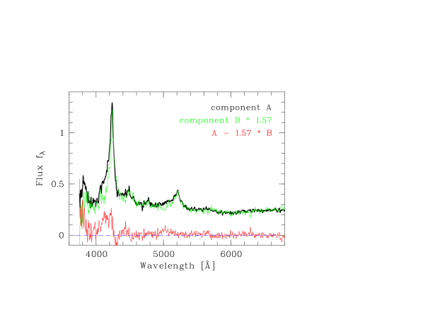
Figure 8: Optical spectra of SDSS J1004+4112  A and B, obtained with PMAS on Calar Alto. For the purpose of comparison, the fainter component B has been scaled to match component A in the continuum. Notice the substantial mismatch in the blue wings of the emission line profiles. See the online edition of the journal for a colour version of this figure.

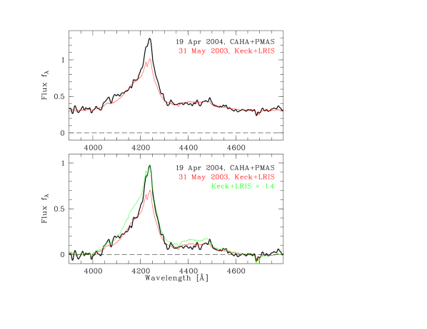
Figure 9: Top panel: Comparison of spectra in the region around the C iv emission line of component A between May 31, 2003 (spectrum kindly provided by Dr. G.T. Richards) and Apr 19, 2004. The almost perfect match in the continuum between the two epochs is not by design and possibly accidental. Bottom panel: Same data, but after subtraction of a local pseudo-continuum, thus underlining the comparison of emission line profiles. Two different scaling factors were explored (see text). See the online edition of the journal for a colour version of this figure.

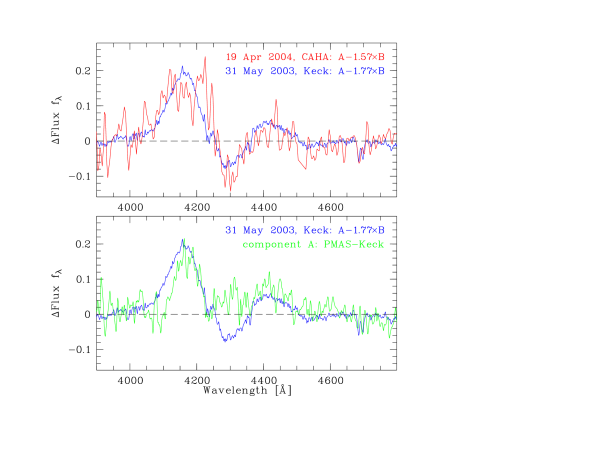
Figure 10: Top panel: Comparison between $f(A)-S\times f(B)$ emission line residuals in the C iv spectral region. Red line: Difference between SDSS J1004+4112  A and B in the PMAS spectra. Blue line: The same for the 2003 Keck spectra. Bottom panel: Green line shows the difference between PMAS and Keck data of component A, compared to the $f(A)-S\times f(B)$ residual for the 2003 Keck spectrum. Please see the online edition of the journal for a colour version of this figure.

5.1 Observations and data reduction

We targeted SDSS J1004+4112  during an observing run on 19 April, 2004, using the Potsdam Multi-Aperture Spectrophotometer PMAS, mounted at the Calar-Alto 3.5 m telescope (Roth et al., 2005). PMAS features a $16\times 16$ elements microlens array coupled to the spectrograph by optical fibres. The image scale is $0\aas@@fstack{\prime\prime}5$ per spatial pixel (‘spaxel’). Because of the limited field of view of $8^{\prime\prime}\times 8^{\prime\prime}$ we only observed components A and B (which fitted easily into one pointing). The spectral resolution was $\sim 6$ Å FWHM, the spectra cover the wavelength range 3800–6800 Å.

Four subsequent exposures of 30 min were obtained. Each was reduced with the procedure described below, after which the spectra were coadded with inverse variance weighting. As the atmospheric transmission during that night turned out to be rather variable, the data are not of absolute spectrophotometric quality. Before coaddition, all exposures were therefore rescaled to match the spectrum with the highest count level. We applied a formal spectrophotometric calibration obtained from observing the standard star HR 3454 immediately before the QSO. Notice that the relative spectrophotometry between components A and B is still very accurate, as there are no geometrical losses due to incomplete coverage of the image plane. (This is different from some other integral-field instruments: The PMAS microlens array reimages the exit pupil of the telescope, and there are therefore no gaps between adjacent fibres.)

The data were reduced using our own IDL-based software package P3d (Becker, 2002). The reduction consists of standard steps such as debiasing and flatfielding using twilight exposures, and dedicated routines such as tracing and extracting the spectra of individual fibres and reassembling the data in form of a three-dimensional data cube. Wavelength calibration and rebinning to a constant spectral increment is also part of the reduction procedure. We extracted the spectra with the iterative fitting method described by Wisotzki et al. (2003). As the seeing was below 1″, the two components of SDSS J1004+4112  did hardly overlap and were easy to deblend despite the coarse spatial sampling. The resulting spectra are shown in Fig. 8.

5.2 Comparison of optical spectra

Already from a superficial examination of Fig. 8 the following facts can be ascertained: (1) The continuum shapes and slopes of components A and B are virtually identical, to the limits of our measurement accuracy. (2) The emission lines do not have identical shapes. The mismatch is easiest seen in the C iv line at $\lambda\simeq 4230$ Å, where component A shows a much stronger blue line wing than component B; qualitatively the same is seen in He ii at $\lambda\simeq 4480$ Å, C iii at $\lambda\simeq 5220$ Å, and also in Si iv at $\lambda\simeq 3890$ Å. Similar mismatches were already observed in previous spectra of the same target by Inada et al. (2003) and Richards et al. (2004). Slit losses in those data, however, prevented a spectrophotometric comparison of the optical continuum. Richards et al. discovered that the strong blue wing excess in the emission lines of component A over B disappeared between May and Nov 2003, after which the A and B spectra were almost (but not quite) identical. Our PMAS data was taken roughly 4 months after the last epoch covered by Richards et al., and here we find that a very similar excess feature is again present. We shall discuss below the implications of this finding in the context of its interpretation as being due to gravitational microlensing.

It is interesting to compare our new spectra directly with those taken at earlier epochs. Dr. G.T. Richards kindly provided us with their previously published spectra in digital form. Of special interest is the May 2003 epoch where the blue wing excess in component A was particularly strong. Fig. 9 shows the spectral region around the C iv and He ii emission lines for component A, as given by the PMAS and Keck datasets. In the top panel, the two spectra are directly superimposed, without any prior rescaling. The two datasets appear to coincide precisely in the continuum, which however could be accidental, since neither dataset is of absolute spectrophotometric quality. In contrast, the C iv emission line equivalent width is roughly 40 % higher in the PMAS data. The line profiles are more readily compared in the bottom panel, where a pseudo-continuum (a straight line fitted to narrow spectral windows at $3920\>\mathrm{\AA}<\lambda<3970\>$Å and $4625\>\mathrm{\AA}<\lambda<4675\>$Å) has been subtracted. After scaling the Keck spectrum by a factor 1.4, the line cores and the red wing of C iv match well, but the blue wing is much more enhanced in the Keck spectrum. The mismatch between PMAS and rescaled Keck data is even more pronounced in He ii.

It thus seems that the blue wing excess has disappeared in the second half of 2003, and reappeared, though weaker, in the first quarter of 2004. We are now interested in the question to what extent this excess flux can be described as a fixed pattern. Indeed we find that the residual spectrum $f(A)-S\times f(B)$, where $S$ is a scaling factor, has a similar shape at both May 2003 and Apr 2004 epochs. This is demonstrated in Fig. 10 (upper panel) where the Keck residuals and the somewhat noisier PMAS residuals agree reasonably well. Another way of pursuing this issue is to ask: Does the blue wing excess $f(A)-S\times f(B)$ have a similar shape as the epoch difference in the emission line spectrum of component A alone? And again we find that this is roughly the case, as shown in the lower panel of Fig. 10. We summarise that the blue wing excess in component A appears to be a recurrent feature that changes its strength, but with a more or less stable spectral shape.

6 Discussion

6.1 Microlensing or intrinsic X-ray variability?

The XMM-Newton  observations of SDSS J1004+4112  reveal strong discrepancies in the optical to X-ray spectral energy distributions of the individual lens images. Furthermore, the optical spectra of image A repeatedly showed enhancements of the blue line wings, which so far have never been observed in any other of the lens images. Two different processes can be considered as the reasons for these deviations: Strong intrinsic flux and spectral variability on timescales comparable to or shorter than the light path time lags between the images can account for both flux and spectral deviations. Microlensing occuring in one or more images can also account in significant flux deviations in the images and can also change the SED of a lens image, if the emission in different wavebands arises in regions of different spatial distribution or extent. This is generally the case for AGN, where the X-ray emission is thought to be emitted from a smaller region in the AGN core than the optical emission, which can be partly attributed to reprocessing in the broad line region.

The fact that both images A and B are so bright in the UV is almost certainly due to intrinsic variablity of the QSO, since the two images separated by the shortest time delay are equally affected. Furthermore it would be very unlikely to find microlensing effects in both images. Also the strong decline of the integral X-ray flux of the object since the epoch of the ROSAT observation, in conjunction with a significant hardening of the X-ray spectrum, is evidence for powerful intrinsic variability.

The low A/B ratio in X-rays could in principle also be a consequence of intrinsic variability coupled with the light path time delay between images A and B, since AGN variability is usually strongest and most rapid in the X-ray regime. However, images A and B are separated by a time lag of only few weeks and at the time of the XMM-Newton observations display a very similar optical to UV SED. These circumstances make intrinsic variability a rather unlikely cause for the observed A/B ratio in X-rays. A microlensing explanation for the low X-ray brightness in component A requires a demagnification in X-rays of a factor $\sim 3$ relative to component B, which seems to be rather extreme. However, Schechter & Wambsganss (2002) calculated microlensing (de-)magnifications for the case of a combination of smoothly distributed matter (i.e. the cluster dark matter in this case) and the matter in stars. Their conclusion is that the dilution of microlensing stellar matter with a smooth component increases the microlensing fluctuations. More specifically, their model predicts a high probability of microlensing demagnifications by 1-2 magnitudes, which is exactly the demagnification required here.

The fact that the inverted A/B ratio was still measured by Chandra in January 2005 (Ota et al., 2006), strengthens our case that it is not caused by intrinsic variability, since the time span between the X-ray observations by far exceeds the possible light path time delay between images A and B. However, the variability of the X-ray A/B ratio, measured at a 2$\sigma$ significance level, may be caused by some intrinsic X-ray variability or a change in the microlensing configuration. The persistently harder X-ray spectrum of image D is most easily explained by intrinsic spectral variability and suggests a time lag of D with respect to the other images of more than 9 month.

6.2 Microlensing of the Broad-Line Region?

As gravitationally lensed images of the same object the two components A and B should have identical spectra, there are only two possibilities to explain the observed spectral differences: On the one hand, the QSO might show rapid intrinsic spectral variability, and the light travel time delay causes some such variations to occur in one component but not in the other. Richards et al. (2004) already made a thoroughly argued case against significant and rapid intrinsic variability, on timescales below the light travel time delay of $\sim 10$–30 days, as the sole origin of the emission line mismatch. We completely agree and merely note that our new observations make this interpretation even less probable, although it is still a formally possible, however unlikely, option.

Alternatively, component A might be suffering from additional microlensing by stars in an intervening galaxy, which could selectively amplify certain regions of the source in a way that the QSO spectrum gets modified (e.g. Schneider & Wambsganss, 1990; Abajas et al., 2002). This was invoked by Richards et al. (2004) to explain the spectral differences between components A and B and the strongly variable emission line profile of component A. The proposed scenario is roughly that a caustic (or a critical curve) moved across only a part of the QSO broad-line region (BLR), amplifiying this particular set of clouds so much that the overall line profile changed temporarily.

A natural prediction of this scenario is that as the caustic pattern continues to move relative to the source, other parts of the source would get amplified, causing further spectral variations. Or possibly the caustic could move away from the compact regions of the source, in which case no more variability would be expected. The one thing that would most certainly not be expected in this scenario is a reoccurence of the same spectral feature, without any other major changes – but this is exactly what we observed. While a cusp caustic could well produce a double-peaked high-amplification pattern, there would always be a leading and a trailing caustic, both of which would act on different parts of the source. We also find that the continuum shapes of components A and B are essentially the same. Thus, the microlensing amplification would have acted on some inner parts of the BLR (because of the high velocity differences relative to the line core), but there would be no chromatic effect on the optical continuum. We cannot think of a reasonable source-caustic configuration that would provide such an amplification pattern.

An alternative explanation of the line variability in SDSS J1004+4112 was recently given by Green (2006), who proposes variable broad line absorption by matter surrounding the QSO. The difference between image A and the other quasar images is explained by the small viewing angle differences, resulting in slightly different light paths through the intervening matter. However, a prediction of this model is significant X-ray absorption with column densities $N_{\rm H}\sim 10^{22}{\rm cm}^{-2}$ in the images B, C, and D, which is clearly ruled out by the XMM-Newton spectra.

We are thus faced with the situation that no simple, single-cause explanation will work. We could either try to construct contrived models of intrinsic variability where substantial variations always happen between the observing gaps. Or we could think of equally contrived models of caustics and a source shape that produce nearly identical differential magnification patterns despite a transverse shift between caustics and source. We reject both and invoke instead, as an act of desperation, a scenario where both intrinsic variability and microlensing play a role. While our proposed scenario certainly deserves being called contrived, our only hope is that it may be somewhat less contrived than the above mentioned options.

The two main reasons to exclude intrinsic variability as the main driver of the differences in the emission lines of SDSS J1004+4112  are: (i) The short light travel time delay in relation to the observed epoch differences; (ii) the huge required variability amplitudes in the wings of the broad lines on these time scales. On the other hand the spectra of component B obtained by Richards et al. (2004) show undeniably that at some moderate level, the optical spectrum of SDSS J1004+4112  does intrinsically change – unless one invokes BLR microlensing for that component as well. Furthermore, these spectral changes may well occur preferentially in the inner regions of the BLR. Now suppose that there is indeed a microlens-induced caustic pattern with high magnification power located such that only a part of the BLR is affected. It would then be that particular part of the BLR that gets highly amplified, and the spectrum would be modified accordingly. But in contrast to the ‘pure microlensing’ scenario, we do not require this caustic pattern to move relatively to the source. In fact, we explicitly wish it to be stationary over the time scales considered. Given the typical effective transverse velocities of several 100 km/s, this seems not unrealistic, probably more realistic than the rapidly moving caustic required in the pure microlensing picture. The only cause for spectral variablity would then be intrinsic line variations, fuelled by the observed X-ray and UV variations. But these intrinsic line variations would be selectively amplified such that always the blue wing of the C iv line, and most of the He ii line, would appear to vary. The Nov/Dec 2003 epoch covered by Richards et al. would then have been a period of relative intrinsic quiescence, while May 2003 and Apr 2004 would have seen a slightly more active BLR.

The possibly best property of this scenario is the fact that it is, in principle, open to empirical testing. If component A is affected by BLR microlensing and component B is not, then all variations in A should have been preceeded (or followed) by much weaker variations in B. The line profile variations need not be similar if the blue wing excess in A is due to the small size of the microlensing region, but the sign of the variations should essentially be the same, and also the relative rates should be in proportion to each other.

7 Conclusions

We have presented simultaneous X-ray observations, UV imaging, and optical spectroscopy of the first QSO lensed by a cluster of galaxies, SDSS J1004+4112 . In all observed bands the observations revealed significant deviations from the simple assumption that all 4 QSO images should have identical spectra and spectral energy distributions: (i) In the optical spectrum of component A the blue wings of the emission lines are brighter than in component B. The same pattern had been observed one year earlier and in the meantime disappeared. (ii) The UV spectra of components A and B are brighter and harder than those of the other components. (iii) In X-rays the flux ratio A/B is a factor of $\sim 3$ lower than in the optical/UV bands.

We show that neither microlensing nor intrinsic variability can be the single cause for all observed anomalies. Instead, we propose a scenario where microlensing is affecting the spectrum of component A. A part of the broad line region, where the blue wings of the lines are emitted, is magnified by microlensing, while the X-ray emitting core of the AGN is demagnified. However, rather than invoking a moving caustic pattern as cause for the line variability, we favour a microlensing situation that remains constant over the timespan of the hitherto performed spectroscopic observations. In our scenario the line variability is caused by flux changes in the UV/X-ray continuum, but the variations are much amplified in the blue line wings of component A because of microlensing. The presence of substantial intrinsic variability can hardly be doubted: For the broad emission lines this is directly seen in the monitoring data by Richards et al. (2004). For the UV continuum it can be inferred from the fact that components A and B have a very similar SED, which in turn differs grossly from that of components C and D. Finally, the X-ray brightness (and spectral shape) has experienced a major change since the epoch of the ROSAT observation.

The microlensing scenario in SDSS J1004+4112  A is special insofar as this line of sight is far away from the lensing galaxy. The surface mass density responsible for the lensing is clearly dominated by smoothly distributed matter in the cluster, on top of which there comes some action from compact bodies (in a cluster galaxy or elsewhere). This is thus an extreme case of the situation envisaged by Schechter & Wambsganss (2002), and we find that the strange observed relative amplification pattern in this source can be well explained in their theoretical scenario. In particular, the most likely ordering of images in arrival time of C-B-A-D makes component A a saddle-point image and therefore more susceptible to microlensing, as was demonstrated by Schechter & Wambsganss (2002).

Due to the relative movement of the intervening galaxy the microlensing caustic pattern is bound to change and the magnifying (and demagnifying) regions of the caustic pattern will move to different emission regions of the AGN. The timescale of this process is governed by the relative transverse velocities of the AGN, the intervening galaxy, and our observer position with respect to each other on the one hand, and the angular scale of the microlensing pattern on the other hand. Assuming the intervening galaxy is a member of the lensing cluster and its velocity is of the order $\sim 1000{\rm km/s}$, its microlensing pattern will cross the angle of one stellar mass Einstein-radius in about 100 years. The magnification patterns calculated by Schechter & Wambsganss (2002) show that the magnifying regions tend to be narrower than the demagnifying regions.

Therefore our proposed scenario predicts for image A that the demagnification of the X-ray source will remain more or less constant for several years. Although the magnifying regions of the caustic patterns are smaller, we also expect the magnification of the blue line wings to change only slowly, since the size of the broad line region is much larger than the X-ray emitting core. Hence, our model predicts further occurences of blue line wing excesses only in image A. However, high SNR spectroscopy should be able to pick up the underlying line flux variations also in the other components.

Obviously a measurement of the time lags at least between images A and B would be extremely helpful to understand the complex behaviour of the system. Our finding that the UV spectrum of the QSO is very variable, suggests that U-band photometry should be a promising method to measure the time lags.