Bright OB stars in the Galaxy

Recent results strongly challenge the canonical picture of massive star winds: various evidence indicates that currently accepted mass-loss rates, ${\dot{M}}$, may need to be revised downwards, by factors extending to one magnitude or even more. This is because the most commonly used mass-loss diagnostics are affected by “clumping” (small-scale density inhomogeneities), influencing our interpretation of observed spectra and fluxes.
Such downward revisions would have dramatic consequences for the evolution of, and feedback from, massive stars, and thus robust determinations of the clumping properties and mass-loss rates are urgently needed. We present a first attempt concerning this objective, by means of constraining the radial stratification of the so-called clumping factor.
To this end, we have analyzed a sample of 19 Galactic O-type supergiants/giants, by combining our own and archival data for H_α, IR, mm and radio fluxes, and using approximate methods, calibrated to more sophisticated models. Clumping has been included into our analysis in the “conventional” way, by assuming the inter-clump matter to be void. Because (almost) all our diagnostics depends on the square of density, we cannot derive absolute clumping factors, but only factors normalized to a certain minimum.
This minimum was usually found to be located in the outermost, radio-emitting region, i.e., the radio mass-loss rates are the lowest ones, compared to ${\dot{M}}$ derived from H_α and the IR. The radio rates agree well with those predicted by theory, but are only upper limits, due to unknown clumping in the outer wind. H_α turned out to be a useful tool to derive the clumping properties inside $r<3{\ldots}5\,R_{\star}$. Our most important result concerns a (physical) difference between denser and thinner winds: for denser winds, the innermost region is more strongly clumped than the outermost one (with a normalized clumping factor of $4.1\pm 1.4$), whereas thinner winds have similar clumping properties in the inner and outer regions.
Our findings are compared with theoretical predictions, and the implications are discussed in detail, by assuming different scenarios regarding the still unknown clumping properties of the outer wind.

1 Introduction

In the last few years, massive stars ($M_{\rm ZAMS}\ga$ 10 ${\rm M}_{\odot}$) have (re-)gained considerable interest among the astrophysical community, in particular because of their role in the development of the early Universe (e.g., its chemical evolution and re-ionization; Bromm et al. 2001, but also Matteucci & Calura 2005). Unfortunately, however, our knowledge of these objects is not as complete as we would like it to be, and present efforts concentrate on modeling various dynamical processes in the stellar interior, as well as in the stellar atmosphere (mass loss, rotation, magnetic fields, convection, and pulsation).

Most important in this regard is the mass loss that occurs through supersonic winds, which modifies evolutionary time-scales, chemical profiles, surface abundances and luminosities. As shown by numerous stellar-evolution calculations, changing the mass-loss rates of massive stars by even a factor of two has a dramatic effect on their evolution (Meynet et al. 1994).

The winds from massive stars in their O-, B- and A-supergiant phase are well described by radiation-driven wind theory (Castor et al. 1975; Pauldrach et al. 1986); the even stronger mass outflows observed during their Wolf-Rayet (WR) and Luminous Blue Variable (LBV) phases are also thought to be driven by radiation pressure (for recent progress, see Gräfener & Hamann 2005 for the case of WRs and Owocki et al. 2005 for LBVs).

Notwithstanding its considerable successes (e.g., Vink et al. 2000; Kudritzki 2002; Puls et al. 2003), the theory is certainly over-simplified. Stellar rotation (e.g., Owocki et al. 1996; Puls et al. 1999 and references therein), and the intrinsic instability of the line-driving mechanism (see below), produce non-spherical and inhomogeneous structure, observationally evident from, e.g., X-ray emission and line-profile variability (for summaries, see Kudritzki & Puls 2000 and Oskinova et al. 2004 regarding the present status of X-ray line emission). As long as the time-dependent structuring of stellar winds is not well understood, we cannot be sure about even their “average” properties, such as mass-loss rates and emergent ionizing fluxes. Even worse, most spectroscopic analyses of hot stars aiming at deriving stellar and wind parameters have been performed by relying on the assumption of a globally stationary wind with a smooth density/velocity stratification. Consequently, the underlying models are incapable in principle of describing the aforementioned features, and the derived results (including the verification of the theory) may depend strongly on this assumption.

Theoretical effort to understand the nature and origin of these observational findings have generally focused on the line-driving mechanism itself; the first linear-stability analyses showed the line force to be inherently unstable (Owocki & Rybicki 1984 and references therein). Subsequent numerical simulations of the non-linear evolution of the line-driven flow instability (for a review, see Owocki 1994), with various degrees of approximation concerning the stabilizing diffuse, scattered radiation field (Owocki & Puls 1996, 1999), have shown that the outer wind (typically, from 1.3 $R_{\ast}$ on) develops extensive structure, consisting of strong reverse shocks separating slower, dense shells from high-speed rarefied regions. Only a very small fraction of material is accelerated to high speed and then shocked; for most of the flow the major effect is a compression into narrow, dense “clumps”, separated by large regions of much lower density.

At first glance, these models appear to be in strong contrast with our assumptions for the “standard model” for wind diagnostics based on stationarity and homogeneity, especially when viewed with respect to the spatial variation of velocity and density. However, when viewed with respect to the mass distribution of these quantities, the models are not so very different (e.g., Owocki et al. 1988; Puls et al. 1993a). Given the intrinsic mass-weighting of spectral formation, and the extensive temporal and spatial averaging involved, the observational properties of such structured models are quite similar to what is derived from the “conventional” diagnostics, in an average sense. Structured winds also explain ‘steady-state’ characteristics like X-rays, and the black absorption troughs observed in saturated UV resonance lines (Lucy 1982, 1983, later confirmed by Puls et al. 1993a on the basis of hydrodynamical simulations).

Recent time-dependent simulations have aimed at investigating two specific problems. First, Runacres & Owocki (2002, 2005) have introduced new methods to numerically resolve even the outermost wind. In particular, they provide theoretical predictions for the radial stratification of the so-called clumping factor,

$$f_{\rm cl}=\frac{<\rho^{2}>}{<\rho>^{2}}\quad\geq 1,$$ (1)

where angle brackets denote (temporal) average quantities. For self-excited instabilities (e.g., without any photospheric disturbances such as pulsations or sound-waves), they find that, beginning with an unclumped wind in the lowermost part ($f_{\rm cl}=1$), the clumping becomes significant ($f_{\rm cl}\simeq 4$) at wind speeds of a few hundreds of km s^-1, reaches a maximum ($f_{\rm cl}\simeq 15{\ldots}20$), and thereafter decays, settling at a factor of roughly four again.

On the other hand, Dessart & Owocki (2003, 2005), building on a pilot investigation by Owocki (1999), have taken the first steps towards including 2-D effects of the radiation field into a higher-dimensional hydrodynamical description, to obtain constraints on the lateral extent of clumping.

Taken together, and with respect to NLTE modeling and spectral analysis, the above scenario has the following major implications, related to radiation field and density/velocity structure:-

1. X-ray emission arising from the formation and interaction of clumps and shocks, in concert with an enhanced EUV flux (e.g., Feldmeier et al. 1997), can have a strong influence on the ionization/excitation balance in the wind (e.g., Pauldrach et al. 2001).

2. Clumping introduces depth-dependent deviations from a smooth density structure, which particularly affects common observational mass-loss indicators, such as H_α emission and the IR/radio excess, since these diagnostics directly depend on $<\rho^{2}>$ (being larger than $<\rho>^{2}$). Furthermore, the ionization balance becomes modified, primarily because of the additional $<\rho^{2}>$-dependence of radiative recombination rates (see also Bouret et al. 2005).

3. Not only the modified density stratification, but also the highly perturbed velocity field can affect the spectral line formation, because of its multiple non-monotonic nature. This gives rise to modified escape probabilities and multiple resonance zones for certain frequencies. A major example of such an influence is the formation of black absorption troughs in saturated UV-resonance lines (see above). Optical lines (e.g., H_α) can also be affected, though to a lesser extent (e.g., Puls et al. 1993b).

Although the potential effects of clumping were first discussed some time ago (e.g., Abbott et al. 1981; Lamers & Waters 1984b; Puls et al. 1993b), and have been accounted for in the diagnostics of Wolf-Rayet stars since pioneering work by Hillier (1991) and Schmutz (1995), this problem has been reconsidered by the “OB-star community” only recently, mostly because of improvements in the diagnostic tools, and particularly the inclusion of line-blocking/blanketing in NLTE atmospheric models.

Repolust et al. (2004) presented results of a re-analysis of Galactic O-stars, previously modeled using unblanketed model atmospheres (Puls et al., 1996), with new line-blanketed calculations. As a result of the line blanketing, the derived effective temperatures were significantly lower than previously found, whereas the modified wind-momentum rates remained roughly at their former values. Based on this investigation, and deriving new spectral-type–$T_{\rm eff}$ and spectral-type–$\log g$ calibrations (see also Martins et al. 2005), Markova et al. (2004, “Paper I”) extended this sample considerably and obtained a “new” empirical wind-momentum–luminosity relationship(WLR; Kudritzki et al. 1995; Kudritzki & Puls 2000) for Galactic O stars, based on H_α mass-loss rates.

Table 1: Sample stars and stellar/reddening parameters as used in this study. Note that radii, mass-loss rates (assuming an unclumped medium) absolute visual magnitudes, M_v, and reddening parameters have been modified with respect to the original values (from “ref1” and “ref2”) by a combined $V/J/H/K$-band de-reddening procedure (see Sect. 2.6), using the indicated distances. Gravitational accelerations, $\log g$, are “effective” values, i.e., without centrifugal correction, derived from H_γ or calibrations; $v_{\rm\infty}$ is in km s^-1; ${\dot{M}}$ is in $10^{-6}\leavevmode\nobreak\ {\rm M_{\odot}/yr}$; and distances are in kpc. “pt” denotes the H_α profile type (emission/absorption/intermediate). “ref1” and “ref2” refer to the sources of the original stellar and magnitude/color/reddening parameters, respectively, where the extensions given for reference “1” denote the “preferred” model chosen in Paper I (see text). For $\zeta$ Pup (HD 66811), we provide two entries, based on different distances (see Paper I).

Star	Sp.Type	$T_{\rm eff}$	$\log g$	$R_{\ast}$	$Y_{\rm He}$	$v_{\rm\infty}$	pt	${\dot{M}}$(opt)	$\beta$(opt)	Mv	E(B-V)	RV	dist	ref1	ref2
Cyg OB2#7	O3If*	45800	3.93	15.0	0.21	3080	e	10.61	0.77	-5.98	1.77	3.00	1.71	2	5
HD190429A	O4If+	39200	3.65	22.7	0.14	2400	e	16.19	0.95	-6.63	0.47	3.10	2.29	1	1-0
HD15570	O4If+	38000	3.50	24.0	0.18	2600	e	17.32	1.05	-6.69	1.00	3.10	2.19	4	6
HD66811	O4I(n)f	39000	3.60	29.7	0.20	2250	e	16.67	0.90	-7.23	0.04	3.10	0.73	3	1-4
				18.6				8.26		-6.23	0.04	3.10	0.46	3	1-0
HD14947	O5If+	37500	3.45	26.6	0.20	2350	e	16.97	0.95	-6.90	0.71	3.10	3.52	3	1-2
Cyg OB2#11	O5If+	36500	3.62	23.6	0.10	2300	e	8.12	1.03	-6.67	1.76	3.15	1.71	2	5
Cyg OB2#8C	O5If	41800	3.73	15.6	0.13	2650	a	4.28	0.85	-5.94	1.62	3.00	1.71	2	5
Cyg OB2#8A	O5.5I(f)	38200	3.56	27.0	0.14	2650	i	11.26	0.74	-6.99	1.63	3.00	1.71	2	5
HD210839	O6I(n)f	36000	3.55	23.3	0.10	2250	e	7.95	1.00	-6.61	0.49	3.10	1.08	3	1-2
HD192639	O7Ib(f)	35000	3.45	18.5	0.20	2150	e	6.22	0.90	-6.07	0.61	3.10	1.82	3	1-0
HD34656	O7II(f)	34700	3.50	25.5	0.12	2150	a	2.61	1.09	-6.79	0.31	3.40	3.20	1	1-6
HD24912	O7.5III(n)((f))	35000	3.50	24.2	0.15	2450	a	2.45	0.80	-6.70	0.33	3.10	0.85	3	1-2
HD203064	O7.5III	34500	3.50	12.4	0.10	2550	a	0.98	0.80	-5.23	0.23	3.10	0.79	3	6
HD36861	O8III((f))	33600	3.56	14.4	0.10	2400	a	0.74	0.80	-5.52	0.08	5.00	0.50	1	1-1
HD207198	O9Ib/II	36000	3.50	11.6	0.15	2150	a	1.05	0.80	-5.15	0.58	2.56	0.83	3	1-1
HD37043	O9III	31400	3.50	17.9	0.12	2300	a	1.03	0.85	-5.92	0.04	5.00	0.50	1	1-1
HD30614	O9.5Ia	29000	3.00	20.7	0.10	1550	e	3.07	1.15	-6.00	0.25	3.10	0.79	3	1-2
Cyg OB2#10	O9.5I	29700	3.23	30.7	0.08	1650	i	2.74	1.05	-6.95	1.80	3.15	1.71	2	5
HD209975	O9.5Ib	32000	3.20	14.7	0.10	2050	a	1.11	0.80	-5.45	0.35	2.76	0.83	3	1-1

References: 1. Markova et al. (2004), 2. Mokiem et al. (2005), 3. Repolust et al. (2004), 4. Repolust et al. (2005), 5. Hanson (2003) (distance from Massey & Thompson (1991)), 6. Mais-Apellaniz et al. (2004).

A comparison of the “observed” wind-momentum rates with theoretical predictions from Vink et al. (2000) and independent calculations performed by our group (Puls et al. 2003), revealed that objects with H_α in emission and those with H_α in absorption form two distinct WLRs. The latter is in agreement with theory, whilst the former appears to be located in parallel, but above the theoretical relation. This difference was interpreted as being a consequence of wind clumping, with the contribution of wind emission to the total profile being significantly different for objects with H_α in absorption compared to those with H_α in emission (since for the former group only contributions from the lowermost wind can be seen, whereas for the latter the emission is due to a significantly more extended volume). Thus, there is the possibility that for these objects one sees directly the effects of a clumped wind, which would mimic a higher mass-loss rate (as is most probably the case for Wolf-Rayet winds). With this interpretation, the presence of clumping in the winds of objects with H_α in absorption is not excluded; owing to the low optical depth, however, one simply cannot see it, and corresponding mass-loss rates would remain unaffected.

The “actual” mass-loss rates for objects with H_α in emission can then be estimated by shifting the observed wind-momentum rates onto the theoretical predictions, with a typical reduction in ${\dot{M}}$ by factors of 2–2.5, corresponding to clumping factors of the order of 4–6.

Though factors between two and three seem reasonable when compared to results from Wolf-Rayet stars (also factors of $\sim$3; e.g., Moffat & Robert 1994), there is increasing evidence that the situation might be even more extreme. From an analysis of the ultraviolet Pv resonance doublet (which is unsaturated, and can therefore be used as a mass-loss indicator), Massa et al. (2003) and Fullerton et al. (2004, 2006) conclude that typical O-star mass-loss rates derived from H_α or radio emission might overestimate the actual values by factors of up to 100 (with a median of 20, if Pv were the dominant ion for spectral types between O4 to O7; see Fullerton et al. 2006). Bouret et al. (2005), from a combined UV and optical analysis, obtained factors between 3 and 7, though from only two stars. In addition, the latter work suggests that the medium is clumped from the wind base on, in strong contrast with typical hydrodynamical simulations (see above). If this were true, presently accepted mass-loss rates for non-supergiant stars also need to be revised, and even the analysis of quasi-photospheric lines (i.e., stellar parameters and abundances) might be affected, since the cores of important lines are formed in the transonic region.

In this paper, we attempt to undertake a first step towards a clarification of the present puzzling situation. From a simultaneous analysis of H_α, IR and radio observations, we obtain constraints on the radial stratification of the clumping factor, and test how far the results meet the predictions given by Runacres & Owocki (2002, 2005). Since all these diagnostics depend on $<\rho^{2}>$, however, we are able to derive only relative, not absolute, values, as detailed in Sect. 4. Let us point out here that our analysis is based upon the assumption of small-scale inhomogeneities redistributing the matter into overdense clumps and an (almost) void inter-clump medium, in accordance with (but not necessarily related to) the basic effects of the line-driven instability. Indeed, the question of whether the wind material is predominantly redistributed on such small scales and not on larger spatial scales (e.g., in the form of co-rotating interaction regions; Mullan 1984, 1986; Cranmer & Owocki 1996) has not yet been resolved, but unexplained residuals from the results of our analysis might help to clarify this issue.

Investigations such as we perform here are not new. Indeed, a number of similar studies have been presented during recent years, e.g., Leitherer et al. (1982); Abbott et al. (1984); Lamers & Leitherer (1993); Runacres & Blomme (1996); Blomme & Runacres (1997); Scuderi et al. (1998); Blomme et al. (2002, 2003). The improvements underpinning our study, which hopefully will allow us to obtain more conclusive results, are related to the following facts. First, and in contrast to earlier work, the uncertainties concerning the adopted stellar parameters have been greatly reduced, since they have been derived by means of state-of-the-art, line-blanketed models. Secondly, we do not derive (different) mass-loss rates from the different wavelength domains based on a homogeneous wind model, but aim at a unique solution by explicitly allowing for clumping as a function of radius, at least in a simplified way. Thirdly, we use recent radio observations obtained with the Very Large Array (VLA), which, because of its gain in sensitivity due to improved performance (mostly at 6cm, where the system temperature improved from 60 to 45 K) allows us to measure the radio fluxes for stars with only moderate wind densities, which produce H_α in absorption. In this way we are able to test the above hypothesis concerning the differences of H_α mass-loss rates from stars with H_α emission and absorption. Lastly, our IR analysis does not depend on assumptions used in previous standard methods exploiting the IR excess (e.g., Lamers & Waters 1984a), since we calibrate against results from line-blanketed NLTE models. (Note that uncertainties in the stellar radii due to distance errors cancel out as far as the derived run of the clumping factors is concerned, and affects “only” the absolute mass-loss rates.)

The plan of this paper is as follows. In Sect. 2, we describe our stellar sample and the observational material used in this study. We also comment on some problems related to reddening. In Sect. 3, we present the methods used to analyze the different wavelength regimes, and discuss how we deal with a clumped wind medium. Applying these methods, we derive constraints for the radial stratification of the clumping factor in Sect. 4, and give a discussion and summary of our findings in Sects. 5 and 6.

2 Stellar sample and observational material

The stellar sample consists of 19 Galactic supergiants/giants, covering spectral types O3 to O9.5. These stars have been analyzed in the optical and, to a large part, (re-)observed by us with the VLA. To our knowledge, the only confirmed non-thermal radio emitter included in our sample is Cyg OB2#8A (Bieging et al., 1989), which was recently detected as an O6I/O5.5III, colliding-wind binary system by de Becker et al. (2004). Somewhat inconsistently, we will use corresponding stellar parameters resulting from an analysis assuming a single star. Note also that HD 37043 is listed as an SB2 binary in the recent Galactic O-star catalogue of Mais-Apellaniz et al. (2004).

Most of the optical analyses were performed by either Repolust et al. (2004) or Mokiem et al. (2005) (Cyg OB2 objects), using the NLTE line-blanketed model-atmosphere code fastwind (Puls et al., 2005). For a few stars (those denoted by “1” in Table 1, column “ref1”), stellar parameters have been derived from calibrations only, as outlined in Paper I. At least for HD 190429A, an independent re-analysis by Bouret et al. (2005), by means of the alternative model-atmosphere code cmfgen (Hillier & Miller, 1998), confirms the corresponding calibration. Finally, for HD 15570, we use parameters derived from $H$- & $K$-band spectroscopy by Repolust et al. (2005).

The parameters adopted in this study are presented in Table 1. For those objects which have been analyzed exclusively in Paper I, and for which more than one choice concerning distance, reddening or luminosity has been discussed, we have used the “preferred” parameter set (Paper I, Table 2), denoted by the corresponding extension in entry “ref 2”. Only for HD 66811 ($\zeta$ Pup) do we provide two entries, referring to its “conventional” distance, $d=460$ pc (2nd entry), and the assumption that this star is a runaway star, located at $d=730$ pc (see Sahu & Blaauw 1993 and Paper I, Sect. 5). Unless stated explicitly, we will use the latter parameter set in our further discussion.

Note that due to minor revisions with respect to reddening, the stellar radii and H_α mass-loss rates (rescaled by assuming $\dot{M}/R_{\star}^{1.5}$ = const, e.g., Puls et al. 1996) for most objects are (slightly) different from the original sources. In Sect 2.6, we will discuss why these revisions were necessary, and how they have been obtained.

2.1 Variability of the diagnostics used

Before we discuss the observations obtained in the individual bands (H_α, IR and radio), let us first give some important comments on the variability of the different diagnostics. Stellar winds are known to be variable on different timescales and in all wavelength ranges in which they are observed. Thus, the use of non-simultaneous measurements, as in our analysis, can be an issue.

Regarding H_α, line profile variations in early-type stars have been observed for years. Since the first extensive surveys by Rosendhal (1973a, b), a large number of investigations have been conducted to establish the properties of the H_α variability and also its origin (e.g., Ebbets 1982; Scuderi et al. 1992; Kaufer et al. 1996; Kaper et al. 1997; Morel et al. 2004). Although the variations in the H_α profile in some cases look very dramatic, they indicate, when interpreted in terms of a variable mass-loss rate, only moderate changes in ${\dot{M}}$, usually not exceeding the uncertainties on the corresponding estimates. Recently, for a sample of 15 O-type supergiants, Markova et al. (2005) constrained the ${\dot{M}}$ variability to about $\pm 4\%$ of the corresponding mean value for stars with stronger winds, and to about $\pm 16\%$ for stars with weaker winds. These estimates are in remarkably good agreement with those from previous studies (Ebbets, 1982; Scuderi et al., 1992) who report variations in ${\dot{M}}$ of about 10 to 30%.

In the case of IR and radio continua, and assuming the emission to be thermal, the timescales of variability (due to variations of micro- or macro-structure, i.e., of the local density or mass-loss rate) can differ by orders of magnitude in the two wavelength regimes. Considering variations in ${\dot{M}}$, the transit time of a front would be of the order of hours in the near-IR forming region (given typical sizes of the emitting region and velocity of the expanding material), and as much as months, or even years, in the radio domain. This implies that whilst the IR emission would display short-term variability, following the mass-loss rate variations very closely, variations in the radio would be averaged out if they occurred on timescales much shorter than the transit time.

Different considerations apply when the variability is of non-thermal origin. In this case, only the radio emission is affected. The process responsible is usually cited as being synchrotron emission (White, 1985), most probably produced in colliding-wind binaries (Van Loo et al., 2006). The main observed characteristics are variability over timescales of up to months, and a power-law spectrum increasing with wavelength and with a variable spectral index (Bieging et al., 1989). In such a case, which is met at least by one of our objects, Cyg OB2#8A, the measured radio-flux(es) can still be used as an upper limit of the thermal free-free emission, by analyzing the lowermost flux measured at the shortest radio wavelength.

Regarding the amplitude of variability, no clear evidence of IR continuum variability has been reported up to now. Amongst the IR observations we have obtained from the literature, there are some studies (e.g., Castor & Simon 1983 or Abbott et al. 1984) with data sampled on timescales ranging from a few hours up to a few months, but no variation of the observed IR fluxes above the errors was reported. If, on the other hand, we compare sets of measurements of the same object, obtained by different authors with different instruments, we do observe differences in the measured fluxes, more likely related to calibration problems than to genuine IR variability (see also Sect. 2.4.1).

With respect to radio emission, there are several pieces of evidence for variability, both in the observed fluxes and in the spectral index. Again, we have to distinguish between thermal and non-thermal emission. In the case of non-thermal origin, variability is always present (e.g., Bieging et al. 1989). This has to be accounted for whenever we have no clear indication about the thermal origin of the observed emission, but where we do see variations. Of our targets, in addition to #8A, this might be a problem only for HD 190429A (and for HD 34656 and HD 37043 for other reasons).

Table 2: VLA radio fluxes (in $\mu$Jy), with 1-$\sigma$ errors in brackets. Data without superscripts are new observations (see Sect. 2.3), whilst data with superscripts correspond to either (a) unpublished measurements by Scuderi et al. or literature values used to complement our database: (b) Scuderi et al. (1998); (c) Bieging et al. (1989); (d) 3.6 cm observations from Lamers & Leitherer (1993) (concerning HD 15570, see text); (e) Blomme et al. (2003, including 20 cm data for $\zeta$ Pup, at 760$\pm$90 $\mu$Jy).
Also indicated are the adopted IR to mm fluxes and the sources from which they have been drawn (see foot of table). Data denoted by “own” refer to $JHKLM$-band observations performed by OGT at the Crimean 1.25 m telescope (see Sect. 2.4). scuba data (at 1.35 mm) were obtained by AWB and IDH (see Sect. 2.5), and scuba 0.85 mm data are from Blomme et al. (2003).

Star	4.86 GHz	8.46 GHz	14.94 GHz	43.34 GHz	IR- and mm-	references
	(6 cm)	(3.5 cm)	(2 cm)	(0.7 cm)	bands used	(IR and mm)
Cyg OB2#7	$<$112	$<$100			$HKLMN$	1,14
Cyg OB2#8A	$<$540a	920(70)a			$JHKLMNQ$	1,5,14,19,20
	1000(200)c		500(200)c
	800(100)c
	700(100)c
	400(100)c
Cyg OB2#8C	$<$200c				$HKLMN$	14
Cyg OB2#10	134(29)	155(26)	300(100)		$JHKLMN$	5,14,19
Cyg OB2#11	182(33)	228(28)	$<$400		$JHKLMN$	5,14
HD 14947	$<$110	$<$135	$<$700		$JHKLMN$	2,5,15,own
	$<90^{a}$	90(30)a
		120(30)a
		110(30)b
HD 15570	100(40)a	220(40)a			$JHKLMNQ$,1.35 mm	1,5,8,11,15,18,scuba
		125(25)d
HD 24912	$<$200	$<$120	$<$390	$<$840	$JHKLMN$,IRAS	3,5,7,16
HD 30614	230(50)b	440(40)b	650(100)b		$JHKLMN$	5,7,own
HD 34656	$<$132	119(24)	$<$510		$JHKL$	17,own
HD 36861	$<$112	$<$90	$<$1000		$JHKLMN$	2,5,7
HD 37043	203(38)	$<$90	$<$330		$JHKLMN$	4,5,16,21,22
		46(15)d
HD 66811	1640(70)e	2380(90)e	2900(300)c		$JHKLM$,IRAS,0.85 mm,1.3 mm	6,9,10,12,13,22,23,24
	1490(110)c
HD 190429A	250(37)	199(36)	$<$420	$<$540	$JHKLM$	5,20,own
		280(30)b
HD 192639		$<$90a			$JHKLM$	5,15,own
HD 203064	114(27)	126(20)	$<$330		$JHKLM$,IRAS	3,5,own
HD 207198	105(25)	101(21)	249(82)		$JHKLM$,IRAS	3,own
HD 209975	165(36)	184(28)	422(120)		$JHKLM$,IRAS	3,own
HD 210839	238(34)	428(26)	465(120)	790(190)	$JHKLMNQ$,IRAS,1.35 mm	1,2,3,5,14,15,own,scuba

References for IR and mm data: 1. Abbott et al. (1984), 2. Barlow & Cohen (1977), 3. Beichman et al. (1988), 4. Breger et al. (1981), 5. Castor & Simon (1983), 6. Dachs & Wamsteker (1982), 7. Gehrz et al. (1974), 8. Guetter & Vrba (1989), 9. Johnson & Borgman (1963), 10. Johnson (1964), 11. Johnson et al. (1966a), 12. Johnson et al. (1966b), 13. Lamers et al. (1984), 14. Leitherer et al. (1982), 15. Leitherer & Wolf (1984), 16. Ney et al. (1973), 17. Polcaro et al. (1990), 18. Sagar & Yu (1990), 19. Sneden et al. (1978), 20. Tapia (1981), 21. The et al. (1986), 22. Whittet & van Breda (1980), 23. Leitherer & Robert (1991), 24. Blomme et al. (2003).

Among thermal emitters, on the other hand, the situation is less clear. There are very few studies which have observed one object several times and at more than one frequency. In the sample studied by Bieging et al. (1989), two from six definite thermal emitters showed variability, both of which are B supergiants (Cyg OB2#12 and $\zeta$ Sco). In these cases, the flux variation reached values of up to 70%. Interpreted in terms of ${\dot{M}}$, this would mean a change of 50% (see Eq. 2). In Scuderi et al. (1998), one out of six objects (again Cyg OB2#12) showed variability whilst having a spectral index compatible with thermal emission. Blomme et al. (2002) studied the variability of $\epsilon$ Ori (B0Ia) and found no evidence for variability, both on shorter and longer timescales. The best-studied object with regard to thermal radio variability is $\zeta$ Pup (O4If+), as a result of the work by Blomme et al. (2003), who investigated both new and various archival data. Again, short-term variability could be ruled out, and long-term variability (with observations beginning in 1978) appeared to be low or even negligible.

The major hypothesis underlying our present investigation (being in agreement with most other investigations performed thus far) is that the clumping properties of a specific wind are controlled by small-scale structures. Further comments on this hypothesis, in connection with the outcome of this analysis, will be given in Sect. 6. If related to any intrinsic wind property (e.g., the instability of radiative line-driving, even if externally triggered by short wavelength/short period modulations), the derived clumping properties should be (almost) independent of time, as long as the major wind characteristics remain largely constant. Accounting for the observational facts above, this assumption seems to be reasonable, and justifies our approach of using observational diagnostics from different epochs. Note also that the observed X-ray variability (where the X-rays are thought to arise mostly from clump-clump collisions) is low as well (Berghöfer et al., 1996), due to the cancellation effects of the large number of participating clumps being accelerated in laterally independent cones (of not too large angular extent, Feldmeier et al. 1997).

If we had analyzed only one object, the derived results might be considered as spurious, of course. However, due to the significant size of our sample, any global property (if present) should become visible. Let us already mention here that our findings, on average, indicate rather similar behaviour for similar objects, and thus we are confident that these results remain largely unaffected by issues related to strong temporal variability.

2.2 H_α observations

For our analysis of H_α by means of clumped wind models, we have used the same observational material as described in Paper I, i.e., H_α spectra obtained at the Coudé spectrograph of the 2m RCC telescope at the National Astronomical Observatory, Bulgaria, with a typical resolution of 15 000. For further information concerning technical details and reduction, see Paper I and references therein.

2.3 Radio observations

New radio observations for 13 stars have been carried out at the VLA (in CnB and C configuration), in several sessions between February and April 2004, for a total of about 36 hours. Some of these stars were already known to be radio emitters, but for many of them only upper limits for their radio emission were available. Exploiting the gain in sensitivity of the VLA, and guided by the requirement of using consistent data at all radio frequencies for our analysis, we decided to (re-)observe them. Note particularly that it was possible to observe not only stars with strong winds, but also those with weaker winds (i.e., with H_α in absorption).

The journal of observations is given in Table 10, with dates, observing frequencies, time on targets, calibrators for flux-density bootstrapping and VLA configuration. The observations were performed with a total bandwidth of 100 MHz at all frequencies. The target stars were observed for several scans of about 10 minutes, interleaved with a proper phase calibrator at 4.86, 8.46, and 14.94 GHz. A faster switching between the target star and the phase calibrator was used at 43 GHz, to remove the rapid phase fluctuations introduced between the antenna elements by the troposphere at this frequency. The data at 15 and 43 GHz have been corrected for atmospheric opacity using a combination of a seasonal model and the surface weather conditions during the experiment. The Astronomical Image Processing System (AIPS) developed by the National Radio Astronomy Observatory (NRAO) was used for editing, calibrating and imaging the data.

Table 2 (left part) displays the corresponding fluxes, together with data from other sources (in most cases, at 2, 3.5 and 6 cm) used to complement our sample. For four objects, partly overlapping with the 13 stars mentioned above, we relied on data (denoted by superscript “a” in Table 2) derived by Scuderi et al. (in preparation), using the VLA in B, BnC and C configuration, in different sessions between 1998 and 1999. The reduction and analysis of these data has been performed in a similar way as outlined above for our new observations. The quoted flux limits for both datasets refer to 3 times the RMS noise on the images, whereas the errors are 1-$\sigma$ errors, again measured on the images. Note that at these low flux densities the contribution of errors introduced by the calibration procedure is negligible.

For the remaining stars, literature values have been used, in particular from Scuderi et al. (1998) and Bieging et al. (1989), together with 3.6 cm observations from Lamers & Leitherer (1993); these are denoted by superscripts “b”, “c” and “d”, respectively. Note that the indicated 3.6 cm flux for HD 15570 deviates from the “original” value of 110$\,\pm\,30$ $\mu$Jy provided by Lamers & Leitherer (1993), as a result of a recent recalibration of the original Howarth & Brown VLA data, performed by IDH. For $\zeta$ Pup, finally, we used the data obtained by Blomme et al. (2003, denoted by superscript “e”), at 3.6 and 6 cm (Australia Telescope Compact Array, ATCA) and 20 cm (VLA), in combination with the 2 cm data from Bieging et al. (recalibrated, see Blomme et al.)

For those objects which have been observed both by us and by others, or where multiple observations have been obtained (particularly for the non-thermal emitter Cyg OB2#8A), we have added these values to our database. In almost all cases, the different values are consistent with each other, especially for the weaker radio sources when comparing with the upper limits derived by Bieging et al. (1989).

2.4 IR observations

Table 3: Near IR magnitudes and errors (last two digits) for program stars as observed with the Crimean 1.25 m telescope.

Star	JD	$J$	$H$	$K$	$L$
	(2453+)				$M$
HD 14947	067.204	7.17 02	6.95 02	6.88 01	6.85 04
	307.456	7.10 01	6.98 01	6.85 04	6.67 08
HD 30614	073.238	4.32 02	4.25 02	4.20 02	4.20 01
	100.224	4.30 01	4.26 01	4.27 01	4.23 01
HD 34656	072.356	6.67 01	6.71 01	6.61 01	6.60 04
	100.244	6.69 02	6.71 01	6.69 01	6.65 03
HD 190429A	216.414	6.28 01	6.12 01	6.14 01	6.13 04
	225.439	6.18 01	6.01 01	6.19 01	5.98 08
HD 192639	216.439	6.45 01	6.24 01	6.22 01	6.26 04
	307.254	6.44 01	6.23 01	6.17 01	6.24 04
HD 203064	223.459	5.17 01	5.12 01	5.13 01	5.13 03
					4.98 10
	311.301	5.19 01	5.17 01	5.17 00	5.02 02
					5.02 05
HD 207198	223.496	5.51 01	5.35 02	5.39 01	5.37 04
					5.58 10
	309.167	5.48 02	5.42 01	5.45 01	5.58 03
					5.57 20
HD 209975	223.535	5.01 01	4.97 01	5.00 01	5.12 05
					5.00 07
HD 210839	223.567	4.62 01	4.52 01	4.54 01	4.57 02
					4.44 05
	309.193	4.61 01	4.51 01	4.58 01	4.62 02
					4.37 06

In the right part of Table 2 we have summarized the IR data used, which are to a large part drawn from the literature. For a few objects, IRAS data for 12, 25, 60 and 100 $\mu$m are also available (Beichman et al., 1988), unfortunately mostly as upper limits for $\lambda\geq$ 25 $\mu$m. For $\zeta$ Pup (HD 66811), however, actual values are present at all but the last wavelength (100 $\mu$m); see Lamers et al. (1984).

For nine objects (denoted by “own” in the “references” column of Table 2), new $JHKLM$ fluxes (see Table 3) have been obtained at the 1.25 m telescope of the Crimean Station of the Sternberg Astronomical Institute (Cassegrain focus, with an exit aperture of 12″), using a photometer with an InSb detector cooled with liquid nitrogen. Appropriate stars from the Johnson catalog (Johnson et al., 1966b) were selected and used as photometric standards. Where necessary, the $HLM$ magnitudes of the standards have been estimated from their spectral types using relations from Koorneef (1983).

2.4.1 Absolute flux calibration

In order to convert the various IR magnitudes from the literature and our own observations into meaningful (i.e., internally consistent) physical units, we have to perform an adequate absolute flux calibration. For such a purpose, at least three different methods can be applied:-

1. Calibration by means of the solar absolute flux, using analogous stars.

2. Direct comparison of the observed Vega flux with a blackbody.

3. Extrapolation of the visual absolute flux calibration of Vega, using suitable model atmospheres.

Although the first two methods are more precise, the latter one provides the opportunity to interpolate in wavelength, allowing the derivation of different sets of IR-band Vega fluxes for various photometric systems. Thus, such an approach is advantageous in the case encountered here (observational datasets obtained in different photometric systems), and we have elected to follow this strategy.

Atmospheric model for Vega.

To this end, we used the latest Kurucz models to derive a set of absolute IR fluxes for Vega in a given photometric system, by convolving the model flux distribution (normalized to the Vega absolute flux at a specific wavelength; see below) with the corresponding filter transmission functions. In particular, we used a model with $T_{\rm eff}$ = 9550 K, $\log g$ = 3.95, [M/H] = -0.5 and $v_{\rm t}$ = 2.0 km s^-1(Castelli & Kurucz, 1994). In order to account for the possibility that the metallicity of Vega might differ from that adopted by us, an alternative model with [M/H] = -1.0 (cf. Garcia-Gil et al. 2005) was used to check for the influence of a different metallicity on the derived calibration. At least for the Johnson photometric system, the differences in the corresponding fluxes turned out to lie always below 1%.

Visual flux calibration.

The most commonly used visual flux calibration for Vega is based on the compilation by Hayes (1985), which has since been questioned by Megessier (1995), who recommends a value being 0.6% larger than the value provided by Hayes (3540 Jy), and equals 3560 Jy (i.e., $3.46\cdot 10^{-9}$ erg cm^-2 s^-1 Å^-1) at $\lambda$ = 5556 Å. This value has been used when normalizing the Kurucz model fluxes to the monochromatic flux at $\lambda$ = 5556 Å. Since the standard error of the Megessier calibration is about one percent, this error is also inherent in our absolute flux distribution.

Vega $V$-band magnitude.

The available $V$-band magnitudes of Vega range from 0 $\aas@@fstack{m}$026 (Bohlin & Gilliland, 2004) to 0 $\aas@@fstack{m}$035 (Colina & Bohlin, 1994), while in the present investigation we adopt $V$ = 0 $\aas@@fstack{m}$03 mag in agreement with Johnson et al. (1966b). With this value, the monochromatic flux for a Vega-like star at the effective wavelength of the $V$ filter is F₅₅₀₀(m_V = 0 $\aas@@fstack{m}$0) = 3693 Jy.

Filter transmission functions.

To calculate the absolute fluxes of Vega in a given photometric system, we have to know the corresponding filter transmission functions, for each band of this system. In those cases where such functions were explicitly available we used them, while for the rest (including our own IR data) we used trapezoidal transmission curves based on the published effective wavelength and FWHM of the filters. The use of trapezoidal instead of actual response functions might, of course, lead to some error in the derived absolute fluxes. Indeed, in the particular case of the ESO filter system, this error was estimated to be less than 5% (Schwarz & Melnick, 1993), with typical values of about 2% systematically larger fluxes from the trapezoidal approximation.

Vega IR magnitudes.

To convert stellar magnitudes into absolute fluxes using Vega as a standard, the magnitudes of Vega in the different filters for the various photometric system have to be known. In our case, these data have been taken from the corresponding literature, and the errors inherent to these measurements are usually very small.

Finally, let us mention that we are aware of the problem that the use of (simplified) model atmospheres for calculating the IR flux distribution of Vega might lead to some uncertainties, as discussed by Bohlin & Gilliland (2004) (e.g., the possibility that Vega is a pole-on rapid rotator, Gulliver et al 1994; Peterson et al. 2004). Note, however, that Tokunaga & Vacca (2005) have recently shown that the near-IR (1 to 5 $\mu$m) absolute flux densities of Vega derived by means of atmospheric models (e.g., Cohen et al. 1992) and by means of direct measurements (e.g., Megessier 1995) are actually indistinguishable within the corresponding uncertainties, which, in these specific cases, are of the order of 1.45% and 2%, respectively.

On the other hand, given the fact that Vega has a dust and gas disk (Wilner et al., 2002) which produces an IR excess, one cannot exclude the possibility that a flux calibration based on a comparison of Vega observed magnitudes and model fluxes might lead to systematic errors, at least for $\lambda\,>5\,\mu$m, as discussed also by Megessier (1995). There are 12 stars in our sample for which we have ground based mid-IR photometry obtained in the $N$- and $Q$-bands. In the case that Vega indeed displays a mid-IR flux excess (as compared to the models), one might expect that the observed fluxes of our targets (based on this calibration) are somewhat underestimated in these bands. Such a systematic error can be easily detected, however, and we shall keep this possibility in mind when performing our analysis.

2.5 Mm observations

For three objects, we were also able to use 1.3/1.35 mm fluxes, acquired either with the Swedish ESO Submillimeter Telescope (SEST) at La Silla ($\zeta$ Pup; see Leitherer & Robert 1991) or with the Submillimetre Common User Bolometer Array (scuba; Holland et al. 1999) at the James Clerk Maxwell Telescope (HD 15570 and HD 210839). (For Cyg OB2#8A, which was also observed with scuba, only badly defined upper limits were obtained.)

The scuba observations were obtained in the instrument’s photometry mode (the standard mode employed for point-like sources), using the single, 1.35 mm photometric pixel, located at the outer edge of the long-wavelength (LW) array. The data were acquired in service mode over the period May–July, 1998. Table 4 lists the observation dates, integration times and measured fluxes. Data reduction was performed using the scuba User Reduction Facility (surf; Jenness & Lightfoot 2000).

Additional 0.85 mm scuba data have been taken from the literature (Blomme et al., 2003), again for $\zeta$ Pup.

Table 4: 1.35 mm fluxes and errors for program stars observed with scuba.

Star	date of obs.	integration (s)	flux (mJy)
Cyg OB2#8A	May 7, 1998	3600	$-2.50\pm 5.95\phantom{-}$
HD 15570	Jul 3, 1998	2160	$4.76\pm 2.43$
HD 210839	May 4, 1998	4500	$4.25\pm 1.92$
	Jun 1, 1998	2340	$8.87\pm 3.58$

2.6 De-reddening and stellar radii

Since we are aiming for a combined optical/IR/radio study, all parameters used have to be consistent in order to allow for a meaningful analysis of the observed fluxes, in particular the excesses caused by the (clumped) wind alone. To compare the observed with the theoretical fluxes, we have ($i$) to de-redden the observed fluxes and ($ii$) to derive a consistent stellar radius for a given distance $d$ (or vice versa, see below), which has been drawn from the literature cited or recalculated from the assumed value of M_v (for models “1-2” in column “ref2” of Table 1).

For this purpose, we have used our (simplified) model as described in Sect. 3.2 to synthesize theoretical $VJHK$ fluxes. Note that this model has been calibrated to reproduce the corresponding predictions obtained from a large OB-model grid calculated by fastwind (Puls et al., 2005).

By comparing the observed IR fluxes (from the various sources given in Table 2) with the theoretical predictions, we derive “empirical” values for the color excess E(B-V) and/or the extinction ratio R_V, by requiring the ratio between de-reddened observed (plus/minus error) and distance-diluted theoretical fluxes to be constant within the $V$- to $K$-bands. For this purpose, we adopt the reddening law provided by Cardelli et al. (1989). Visual fluxes have been calculated using $V$-magnitudes from Paper I or from Mais-Apellaniz et al. (2004).

In a second step, we adapt the stellar radius (for a given distance) in such a way that the mean ratio becomes unity. This procedure ensures the correct ratio between radius and distance, i.e., angular diameter, which is the only quantity which can be specified from a comparison between synthetic and observed fluxes. Of course, we could have also chosen to modify the distance for a given radius; however, in order to be consistent with previous mass-loss estimates from radio observations, which rely on certain distances, we have followed the former approach. Fig. 1 gives an impression of this procedure, for the example of Cyg OB2#8A.

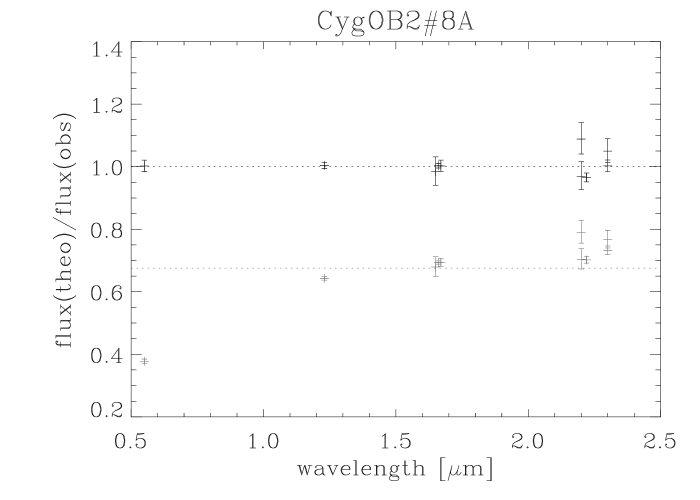
Figure 1: De-reddening procedure, for the example of Cyg OB2#8A. Displayed is the ratio of distance-diluted, theoretical fluxes and de-reddened, observed $VJHK$ fluxes, as a function of wavelength, with bars accounting for the observational errors. Grey entries correspond to “fit-parameters” E(B-V) = 1.9, R_V = 3.0 and $R_{\ast}$ = 24 $R_{\odot}$. Obviously, the extinction is too large: the ratio of theoretical to de-reddened fluxes is much smaller at shorter than at larger wavelengths (extinction decreasing with wavelength). Moreover, the assumed radius is too small, since the mean flux ratio (indicated by a dotted line) is well below unity (too small an angular diameter). The black entries show our final solution, for E(B-V) = 1.63, R_V= 3.0 and $R_{\ast}$= 27 $R_{\odot}$. Any curvature has vanished, the optical flux corresponds to the mean, and the mean ratio itself (again indicated by a dotted line) is located at unity.

Note that in parallel with re-defining the stellar radius, the mass-loss rate used to calculate the $V$- to $K$-band model fluxes has to be modified as well, because the latter depend on the assumed value of ${\dot{M}}$ (see below). Since we do not know the actual mass-loss rate in advance, we follow a simplified approach and use a value equal or related to the H_α mass-loss rate provided by previous investigations (entry “ref1”). This mass-loss rate, however, had been derived for a certain stellar radius, which we claim to improve by our procedure. Consequently, we also have to modify our “input value” of ${\dot{M}}$, to maintain the H_α fit-quality of the former investigations. As outlined already above, this can be obtained by keeping the ratio $Q^{\prime}=\dot{M}/R_{\star}^{1.5}$ constant.

This scaling has a further advantage, namely that not only H_α  but all $\rho^{2}$-dependent diagnostics (i.e., H_α profile shape, IR and radio fluxes) and the finally derived run of the clumping factor remain almost unaffected if a different radius or distance (though identical angular diameter) are chosen.

This notion follows from the fact that the H_α profile shape depends on $Q^{\prime}$ alone (for given $v_{\rm\infty}$ and assuming that the NLTE departure coefficients do not vary), and that the IR and radio optical depths scale with this quantity as well, whereas the corresponding fluxes are additionally diluted by $(R_{\star}/d)^{2}$. As an example, remember that under certain conditions (see Sect 3.3) the radio fluxes scale according to

$$F_{\nu}\propto\frac{\dot{M}^{4/3}}{d^{2}}\,=\,\bigr{(}\frac{\dot{M}}{R_{\star}^{3/2}}\bigl{)}^{4/3}\,\bigr{(}\frac{R_{\star}}{d}\bigl{)}^{2}.$$ (2)

In other words, as long as $Q^{\prime}$ and the angular diameter (“measured” from aligning synthetic and observed, de-reddened fluxes; see Fig. 1) remain conserved, almost all further results become independent of the individual choice of $R_{\ast}$ or $d$, and a translation of our results to different assumptions, e.g., due to future improvements concerning distance measurements (gaia), becomes easily possible. The only quantities which depend directly on these values are the mass-loss and wind-momentum rate (e.g., Paper I), which are of minor importance regarding the objectives of this paper.

One problem inherent to our approach is the fact that the derivation of reddening parameters and $R_{\ast}$ requires an a priori knowledge of ${\dot{M}}$ (and clumping properties), since, as stated already above, the model fluxes depend on this quantity.

First note that the flux excess increases as a function of ${\dot{M}}$. Consequently, the average slope of the model fluxes decreases, which affects our de-reddening procedure (operating in the $V$- to $K$-band). This dependence, however, is only moderate, due to the rather low excess in this wavelength region for typical OB-star winds. Moreover, it is predicted correctly by our models if $Q^{\prime}$ is of the correct order.

The absolute flux level in the optical and near IR, on the other hand, is much more affected by our choice of ${\dot{M}}$, thus influencing our derivation of $R_{\ast}$. For identical stellar parameters, the $V$-flux is a (monotonically) decreasing function of ${\dot{M}}$. To a large extent, this behaviour is induced by a decreasing source function at bf-continuum formation depth, related to the decrease in electron temperature (at $\tau(\dot{M})\approx 2/3$) when ${\dot{M}}$ is increasing, and increasing electron scattering. Both effects apply to blanketed and unblanketed models; the “only” difference concerns the absolute flux level at optical and (N)IR bands, which is larger for blanketed models, due to flux-conservation arguments (compensation of the blocked (E)UV radiation field).

Since a precise knowledge of the “real” wind density and the near-photospheric clumping properties is not possible at this stage, only an iteration cycle exploiting the results of our following mass-loss/clumping analysis could solve the problem “exactly”.

In order to avoid such a cycle, we follow a simplified approach, in accordance with our findings from Paper I and anticipating our results from Sect. 4 (cf. column “ratio” in Table 7). To calculate the theoretical fluxes required for our de-reddening procedure, for objects with H_α in absorption we have used the actual, $Q^{\prime}$-scaled, H_α mass-loss rate, whereas for objects with H_α in emission we have reduced the corresponding value by a factor of 0.48. This approach is based on our hypothesis that the lowermost wind is unclumped (see Sect. 3.4), and that the previously derived H_α mass-loss rates for objects with H_α in emission are contaminated by clumping, with average clumping factors of the order of $\bigl{(}\frac{1}{0.48}\bigr{)}^{2}$.

From the almost perfect agreement of the theoretical $V$-to-$K$ fluxes with the observations for our final, clumped models, this assumption seems to be fairly justified. In any case (i.e., even if the lowermost wind were to be clumped as well), the most important quantity is the effective mass-loss rate (i.e., the actual, unclumped ${\dot{M}}$ times square root of local clumping factor), so any reasonable error regarding this quantity would barely affect the corresponding theoretical fluxes and thus our de-reddening procedure.

We will now comment, where appropriate, on the results of our procedure for a few individual objects. For the majority of stars, only small modifications of the E(B-V) values resulting from optical photometry, $(B-V)$, and intrinsic colors, $(B-V)_{0}$, were necessary, while keeping the total-to-selective extinction ratio, R_V, at its “normal” value of 3.1, or at a value suggested from other investigations. The intrinsic colors used here have been adapted from Wegner (1994), particularly because of their extension towards hotter spectral types. However, since this calibration deviates considerably from the widely used alternative provided by Fitzgerald (1970) at the cool end (-0.24 mag vs. -0.28 mag for O9.5 supergiants), we adopt, as a compromise, only values $\leq-0.27$, and $-0.27$ if Wegner’s calibration exceeds this threshold.

Concerning the Cyg OB2 stars, for three objects (#7, #8A and #8C), our procedure results in rather similar reddening parameters to those presented by Hanson (2003, based on UBV photometry by Massey, priv. comm., and IR-photometry from 2MASS). Only for stars #10 and #11 did we find larger discrepancies, which were corrected for by using R_V = 3.15 instead of R_V = 3.0, as suggested by Hanson and previous work in the optical (Massey & Thompson 1991; Torres et al. 1991). Note that “our” value is consistent with the values provided by Patriarchi et al. (2003, see below): R_V = 3.17 and 3.18, respectively.

Figure 2: Differences between derived color excess, E(B-V), and corresponding literature value, $(B-V)-(B-V)_{0}$ (Table 1, entry “ref 2”; for intrinsic colors see text), as a function of $T_{\rm eff}$. Asterisks denote supergiants, and crosses bright giants and giants, respectively. The mean deviation for supergiants is $-0.004\,\pm\,0.016$ mag, and for l.c. II/III stars $-0.01\,\pm\,0.023$ mag.

In disagreement with the work by Hanson, however, we still used the canonical distance of $d=1.71$ kpc for the Cyg OB2 stars, as determined by Massey & Thompson (1991). In our opinion, the alternative, lower value(s) claimed by Hanson would result in too low luminosities. Most probably, though, the “real” distance is smaller than the value used here. As pointed out, this would imply “only” a down-scaling of radii and mass-loss rates, and would not affect our conclusions concerning the wind clumping.

The only other objects worthy of closer inspection are those with extinction ratios R_V $\neq 3.1$ (cf. Paper I). Unfortunately, the recent catalogue of R_V values for Galactic O-stars by Patriarchi et al. (2003) covers only few stars in our sample (in particular, Cyg OB2#8A, #10, #11 and HD 34656), such that a comparison is not possible for the majority of objects. Due to the degeneracy of E(B-V) and R_V (different combinations can result in rather similar extinction laws, if the considered wavelength range is not too large), we applied the following philosophy: in those cases with peculiar extinction ratios, R_V $\neq 3.1$, (obtained from Paper I and references therein), we firstly checked, by using these values, whether the derived color excess is consistent (within small errors; see below) with measured and intrinsic colors in the optical. If so, we adopted these values here. In this way, we confirmed the values of R_V = 5.0, 5.0 and 2.76 for the stars HD 36861, HD 37043 (both belonging to Ori OB1) and HD 209975, respectively.

For HD 207198, with a literature value of R_V =2.76, the derived color excess would have fallen 0.04 mag below the “optical” value (a deviation which we considered to be too large if R_V $\neq$3.1 anyway). Therefore, for this object, we kept the optical E(B-V) value and fitted R_V using our procedure, resulting in R_V = 2.56. This star is the only one for which our procedure showed significant deviations from previous work. Given the difficulties in deriving reliable R_V values, however, we consider this deviation as not too troublesome.

For the last object in this group, HD 34656, we could check for the consistency of our results with the work by Patriarchi et al. By keeping R_V = 3.1, as suggested in Paper I, the derived E(B-V) would lie 0.03 mag above the “optical” value, which, compared to the other objects (see below), is rather large. On the other hand, by keeping our value of E(B-V), we derived R_V = 3.4, which is consistent with the value claimed by Partriarchi et al. (R_V = 3.5), and we adopted this solution.

Fig 2 summarizes the results of our de-reddening procedure, by comparing the derived values of E(B-V) for our complete sample with the corresponding “optical” values, $(B-V)-(B-V)_{0}$, as a function of $T_{\rm eff}$ (with (B-V) given by the references in Table 1, entry “ref 2”, and the intrinsic colors as discussed above).

From this figure, we find no obvious trend of the difference in E(B-V) as a function of $T_{\rm eff}$ (the average differences being almost exactly zero for supergiants and $-0.01$ mag for the remaining objects), which is also true if we plot this quantity as a function of M_v (not shown). The majority of these differences are less than $0.02$ mag, which seems to be a reasonable value when accounting for the inaccuracy in the observed $(B-V)$ colors, the uncertainties in the intrinsic ones, the errors resulting from our flux calibration and the typical errors on the theoretical fluxes (cf. Sect. 3.2).

3 Simulations

In this section, we will describe our approach to calculating the various energy distributions required for our analysis, and our approximate treatment of wind clumping, which is based upon the assumption of small-scale inhomogeneities. Since this treatment consists of a simple manipulation of our homogeneous models, we will start with a description of these.

Because of the large number of parameters to be varied (${\dot{M}}$, $\beta$, clumping factors), and accounting for the rather large sample size, an “exact” treatment by means of NLTE atmospheres is (almost) prohibitive. Thus, we follow our previous philosophy of using approximate methods, which are calibrated by means of our available NLTE model grids (Puls et al., 2005), to provide reliable results. Note that these grids have been calculated without the inclusion of X-rays; the influence of X-rays on the occupation numbers and IR/radio opacities of hydrogen is negligible (e.g., Pauldrach et al. 2001), whilst their effect on helium (through their EUV tail) has not been investigated in detail. From a comparison of models with and without X-rays though, any effect seems to be small.

We have been able to design interactive procedures (written in idl acting as a wrapper around fortran-programs), which allow for a real-time treatment of the problem, where all required fits and manipulation of H_α spectra and IR/radio fluxes are obtained in parallel.

3.1 H_α

Table 5: Consistency check for H_α mass-loss rates and velocity field exponents, for those objects with stellar and wind parameters derived from a complete NLTE analysis (cf. Table 1). All mass-loss rates are in units of of $10^{-6}{\rm M_{\odot}/yr}$. $\dot{M}_{1}$ is the mass-loss rate as derived from our approximate method, adopting $\beta_{1}=\beta$(in), where possible. In some cases, a second solution ($\dot{M}_{2},\beta_{2}$) is possible, mostly for objects with H_α in absorption (see text).

Star	${\dot{M}}$(in)	$\beta$(in)	$\dot{M}_{1}$	$\beta_{1}$	$\dot{M}_{2}$	$\beta_{2}$
Cyg OB2#7	10.61	0.77	${\dot{M}}$(in)	$\beta$(in)	9.5	0.90
HD 15570	17.32	1.05	16.00	$\beta$(in)	${\dot{M}}$(in)	0.95
HD 66811	16.67	0.90	13.50	$\beta$(in)
	8.26	0.90	6.69	$\beta$(in)
HD 14947	16.97	0.95	${\dot{M}}$(in)	$\beta$(in)
Cyg OB2#11	8.12	1.03	9.50	1.10
Cyg OB2#8C	4.28	0.85	3.50	1.00
Cyg OB2#8A	11.26	0.74	13.00	$\beta$(in)	${\dot{M}}$(in)	0.95
HD 210839	7.95	1.00	${\dot{M}}$(in)	$\beta$(in)
HD 192639	6.22	0.90	5.70	1.14	${\dot{M}}$(in)	1.05
HD 24912	2.45	0.80	4.00	$\beta$(in)	${\dot{M}}$(in)	1.05
HD 203064	0.98	0.80	1.30	$\beta$(in)	${\dot{M}}$(in)	0.92
HD 207198	1.05	0.80	1.30	$\beta$(in)	${\dot{M}}$(in)	0.90
HD 30614	3.07	1.15	2.40	$\beta$(in)
Cyg OB2#10	2.74	1.05	3.30	$\beta$(in)
HD 209975	1.11	0.80	1.20	0.90

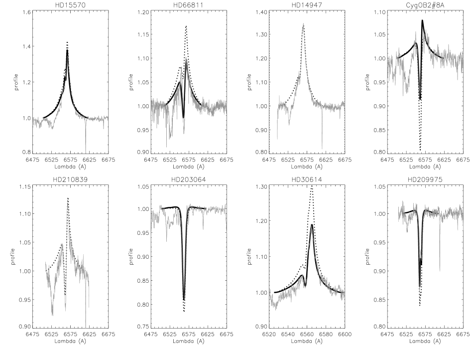
Figure 3: Consistency check for H_α profiles: results of our approximate H_α line synthesis, for some representative cases from Table 5. Dotted: H_α line profiles with parameters ${\dot{M}}$(in) and $\beta$(in) as derived from a complete NLTE analysis (cf. Table 1); bold: corresponding profiles with ${\dot{M}}$ = $\dot{M}_{1}$ or $\beta=\beta_{2}$ (see Table 5).

In the present study, synthetic H_α profiles are calculated as described in Paper I. This approach bases on the approximate treatment as introduced by Puls et al. (1996), updated to account for line-blanketing effects. Except for the inclusion of clumping, no further modifications have been applied; note in particular that we have used the same H_α observations and H/He departure coefficients as adopted in Paper I.

On the other hand, for most of our sample stars we have quoted (and used, within our de-reddening procedure) wind parameters from a complete NLTE analysis, which do not rely exclusively on H_α, but also on Heii 4686 and other diagnostics. Furthermore, the observed H_α profiles used here are different to those in the corresponding sources, because of the variability of H_α (cf. Sect. 2.1). Thus, we have to check how far the values from the complete analysis (denoted by ${\dot{M}}$(in) and $\beta$(in)) might deviate from solutions resulting from our simplified method, used in combination with our different H_α data, to obtain consistent initial numbers for the following investigations and to re-check the reliability of our approach. To this end, we have re-determined mass-loss rates and velocity exponents, using our observational material, the stellar parameters from Table 1 and the approximate H_α line synthesis as outlined above. Table 5 summarizes the results from this exercise.

For three objects (Cyg OB2#7, HD 14947 and HD 210839), no modifications were required at all, whereas for the other stars small variations of ${\dot{M}}$ were sufficient to reproduce our observational data, mostly by keeping the nominal velocity exponent. The average ratio between modified and input mass-loss rates was 1.07 $\pm$ 0.22.

In some cases (particularly for objects with H_α in absorption), a second solution is possible, and in all but one case, we kept the nominal mass-loss rate constant, while varying $\beta$ (entry $\beta_{2}$ in Table 5). All derived velocity exponents still lie in the expected range. For representative cases, Fig. 3 displays the results of our line synthesis, both for models with the nominal values, ${\dot{M}}$(in) and $\beta$(in), and for the best-fitting models from Table 5, with $\dot{M}_{1}$ or $\beta_{2}$.

In conclusion, our simplified routine delivers reliable numbers and thus can be used in our further approach to derive constraints on the clumping factors.

3.2 Infrared fluxes

For the calculation of the infrared fluxes, we closely followed the approximations as outlined by Lamers & Waters (1984a), with Gaunt factors from Waters & Lamers (1984). The major difference concerns the fact that the radiative transfer is solved by means of the “Rybicki algorithm” (Rybicki, 1971), to account for electron scattering in a convenient way.

A further modification regards the photospheric input fluxes which were chosen in such a way as to assure that the emergent fluxes, on average, comply with the results from our detailed NLTE model grids.

After some experiments, it turned out that the best choice for the various parameters is the following:-

The velocity law

is specified by

$$v(r)=v_{\infty}(1-b/r)^{\beta},\qquad b=1-(v_{\rm min}/v_{\infty})^{1/\beta},$$ (3)

where $r$ is calculated in units of $R_{\ast}$, and the minimum velocity, $v_{\rm min}$, is set to 10 km s^-1.

Electron temperature.

All Gaunt factors are calculated at a temperature of 0.9 $T_{\rm eff}$, and the electron temperature is calculated using Lucy’s temperature law for spherical atmospheres (Lucy, 1971, his Eq. 12, and using grey opacities), with an optical depth scale accounting for electron scattering only and a temperature cut-off at 0.5 $T_{\rm eff}$. Remember that the radio fluxes are almost independent of the temperature, and a number of tests have shown that different (reasonable) temperature stratifications have negligible effects on the derived IR fluxes as well.

Ionization equilibrium.

Hydrogen is assumed to be (almost) completely ionized, helium as singly ionized outside the recombination radius (see below) and the CNO metals as either two or three times ionized.

Throughout the parameter range considered here, helium is singly ionized in the radio emitting region (for $\lambda>2$ cm; concerning mm fluxes see below), as we have convinced ourselves by an inspection of our model grid. (Only for O3/4 dwarfs and earlier types – which are missing in our sample – does helium remain completely ionized throughout the entire wind).

Figure 4: Location of Heiii recombination in velocity space (in units of $v_{\rm\infty}$), as a function of $T_{\rm eff}$. Crosses display this location as derived from our model grid, with 27.5 kK $\leq T_{\rm eff}\leq$ 47.5 kK, different gravities and wind densities. Curves indicate the results of our linear regression, Eq. 4, for the (limiting) cases ($\log g$=3.0, $\bar{\rho}=-13$, solid), ($\log g$=3.0, $\bar{\rho}=-11$, dotted), ($\log g$=4.5, $\bar{\rho}=-13$, dashed) and ($\log g$=4.5, $\bar{\rho}=-11$, dashed-dotted). For units of $\bar{\rho}$, see text. The only region which is not matched by our regression is the low gravity, low wind density region around $T_{\rm eff}$= 33,000 K, where the regression yields too low recombination velocities.

With respect to the mid- and far-IR emitting region, this statement is no longer justified, and one would have to calculate a consistent ionization structure, which is beyond the scope of this paper. In order to obtain an approximate solution of this problem, we have parameterized the recombination radius, in dependence of $T_{\rm eff}$, $\log g$ and mean wind density, $\bar{\rho}=\dot{M}/(R_{\star}^{2}v_{\infty})$, from a linear regression to corresponding results of our model grid (cf. Fig. 4, crosses). It turned out that a best fit could be obtained for the recombination velocity (defined as the velocity where the ionization fraction of Heiii becomes larger than the fraction of Heii when proceeding from outside to inside), which can expressed (in units of $v_{\rm\infty}$) as

$$v_{\rm rec}=c+a_{1}\log T_{\rm eff}+a_{2}\log g+a_{3}\log\bar{\rho},$$ (4)

$${\rm min}(v_{\rm rec})=0,\qquad{\rm max}(v_{\rm rec})=1,$$

with

$$27,500\,{\rm K}<T_{\rm eff}<35,000\,{\rm K}:$$

$$c=-34.60\,\,a_{1}=7.79\,\,a_{2}=-0.3325\,\,a_{3}=-0.0854$$

$$37,500\,{\rm K}<T_{\rm eff}<47,500\,{\rm K}:$$

$$c=-14.90\,\,a_{1}=3.31\,\,a_{2}=-0.0956\,\,a_{3}=-0.0798,$$

where $T_{\rm eff}$ is measured in K, ${\dot{M}}$ in ${\rm M}_{\odot}$/yr, $R_{\ast}$ in $R_{\odot}$ and $v_{\rm\infty}$ in km s^-1. For $35{\rm k}K<T_{\rm eff}<37.5{\rm k}K$, we have applied a linear interpolation.

Concerning the models of our grid, this relation results in a mean difference, $\langle v_{\rm rec}$(Eq. 4)-$v_{\rm rec}$(model)$\rangle=0.011\pm 0.079$ (in units of $v_{\rm\infty}$), where the largest discrepancies are found in the low gravity, low wind density region around $T_{\rm eff}$ = 33,000 K (cf. Fig. 4). Note that for high gravity, $\log g$ = 4.5, and low wind density, $\log\bar{\rho}=-13.0$ (dashed line), the complete wind contains solely Heii for $T_{\rm eff}\la$ 31,000 K, whereas for low gravity, $\log g$ = 3.0, and high wind density, $\log\bar{\rho}=-11.0$ (dotted line), it remains completely ionized for $T_{\rm eff}\ga$ 42,000 K. For our final model of $\zeta$ Pup (HD 66811), our approximation yields $v_{\rm rec}=0.87$, which is in good agreement with the value of $v_{\rm rec}=0.83$ found by Hillier et al. (1993) in their paper on the X-ray emission of this object.

Mostly affected by the presence of Heiii (compared to the assumption that helium is singly ionized throughout the wind) is the mid and far IR-band, where the effective photosphere might be located below the recombination radius. (In the near-IR, the emitted flux is still dominated by the “real” photosphere.) Except for a few objects, the former wavelength range has not been observed so far, so that our predictions remain to be verified in the future. Note finally that from the scaling relations provided by, e.g., Lamers & Waters (1984a), the difference in the derived mass-loss rates (using Heiii instead of Heii as the major ion, i.e., no recombination at all) would result in a factor of roughly 0.85 for solar helium content. Further comments on the influence of the helium ionization balance will be given in Sect. 4.1.

Photospheric input fluxes

were chosen as follows: For $\lambda<1\,\mu{\rm m}$, we used Kurucz fluxes, whereas for higher wavelengths we used Planck functions with $T_{\rm rad}$= 0.87 $T_{\rm eff}$ for $1\,\mu{\rm m}\leq\lambda\leq 2\,\mu{\rm m}$, $T_{\rm rad}$= 0.85 $T_{\rm eff}$ for $2\,\mu{\rm m}\leq\lambda\leq 5\,\mu{\rm m}$ and $T_{\rm rad}$= 0.9 $T_{\rm eff}$ elsewhere. Note that for considerably larger wavelengths, the emergent fluxes become independent of the input fluxes, due to increasing optical depths.

We have compared the fluxes resulting from this simplified model with those from our NLTE model grid as calculated by fastwind, for the wavelength bands $V$ to $Q$. (A comparison beyond 30 $\mu{\rm m}$ is not possible, since this is the maximum wavelength considered in fastwind, which follows from the constraint that, for all IR wavelengths and all wind densities, the wind plasma should become optically thick only well inside the outermost radius point, $R_{\rm max}$ = 100 $R_{\ast}$.)

For this comparison, 204 models within the range 30 kK $\leq T_{\rm eff}\leq$ 45 kK, with different gravities and wind densities (corresponding to $\log Q=\log(Q^{\prime}/v_{\infty}^{1.5})$ = -13.15…-12.1, if $v_{\rm\infty}$ is calculated in km s^-1, see Puls et al. 2005, Sect. 10) have been used. As a result, the mean ratio of IR fluxes from our simplified model to those from fastwind is of the order of 0.99…1.01 (different for different wavelengths), and the typical standard deviation for each wavelength band is below 5%.

3.3 Radio fluxes

Radio fluxes are calculated in analogy to the IR fluxes (with identical parameters), but neglecting electron scattering. We use a numerical integration, with $R_{\rm max}$ = 10,000 $R_{\ast}$, for the following reasons: first, the analytical expression by analogy to Eq. 2, as provided by Panagia & Felli (1975) and Wright & Barlow (1975), is valid only under the condition that the plasma is already optically thick at $v(r)\approx v_{\infty}$, which is not the case for objects with thin winds. Secondly, the inclusion of depth-dependent clumping factors requires a numerical integration anyway. Of course, we have checked that for constant clumping factors and large wind densities, the analytical results are recovered by our approach. Remember that the emitted fluxes are almost independent of the assumed electron temperature. From our final results, it turned out that except for the mm fluxes of our hottest objects, Cyg OB2#7 and HD 15570, the radio photospheres of the complete sample (even if sometimes below $v_{\rm\infty}$) are well above the corresponding recombination radius (cf. Table 7). Thus, unless explicitly stated otherwise, helium is adopted to be singly ionized in our radio simulations. In the following figures, the radio range is indicated to start at 400 $\mu{\rm m}$ = 0.4 mm (end of IR treatment at 200 $\mu{\rm m}$), but this serves only as a guideline, since at these wavelengths helium might still not be completely recombined.

3.4 Inclusion of wind clumping

To account for the influence of wind clumping, we follow the approach as described by Abbott et al. (1981). Modified by one additional assumption (see below), this approach has been implemented into NLTE model atmospheres already by Schmutz (1995), and is presently also used by the alternative NLTE code cmfgen. In the following, we will recapitulate the method and give some important caveats.

Regarding the hydrodynamical simulations of radiatively driven winds, the term “clumping factor” has been introduced by Owocki et al. (1988), as defined from the temporal averages in Eq. 1. To allow for a translation to stationary model atmospheres, one usually assumes that the wind plasma is made up of two components, namely dense clumps and rarefied inter-clump material, in analogy to snapshots obtained from the hydrodynamics. The volume filling factor, $f$, is then defined as the fractional volume of the dense gas, and one can define appropriate spatial averages for densities and density-squares (cf. Abbott et al. 1981),

$$<\rho> = \frac{1}{\Delta V}\int\bigl{[}f\rho^{+}\,+\,(1-f)\,\rho^{-}\bigr{]}{\rm d}V$$ (5)

$$<\rho^{2}> = \frac{1}{\Delta V}\int\bigl{[}f(\rho^{+})^{2}\,+\,(1-f)\,(\rho^{-})^{2}\bigr{]}{\rm d}V,$$ (6)

where $\rho^{+}$ and $\rho^{-}$ denote the overdense and rarefied material, respectively. Here, and in the following, we have suppressed in our notation any spatial dependence, both of these quantities and of $f$. The actual mass-loss rate (still assumed to be spatially constant, in analogy to the temporal averaged mass-loss rate resulting from hydrodynamics) is then defined from the mean density,

$$\dot{M}=4\pi r^{2}<\rho>v,$$ (7)

and any disturbance of the velocity field (e.g., influencing the line-transfer escape probabilities; see Puls et al. 1993a) is neglected.

The modification introduced by Schmutz (1995) relates to the results from all hydrodynamical simulations collected so far, namely that the inter-clump medium becomes almost void after the instability is fully grown, i.e, outside a certain radius. In this case then, $\rho^{-}$ $\rightarrow$  0, and we find, assuming sufficiently small length scales (see below),

$$<\rho> = \frac{1}{\Delta V}\int\bigl{[}f\rho^{+}\bigr{]}{\rm d}V\,=\,f\rho^{+}$$ (8)

$$<\rho^{2}> = \frac{1}{\Delta V}\int\bigl{[}f(\rho^{+})^{2}\bigr{]}{\rm d}V\,=\,f(\rho^{+})^{2}\,=\,\frac{<\rho>^{2}}{f}.$$ (9)

Comparing with Eq. 1 and identifying temporal with spatial averages, we obtain

$$f_{\rm cl}=\frac{1}{f}\qquad{\rm and}\qquad\rho^{+}=\frac{<\rho>}{f}\,=\,f_{\rm cl}<\rho>,$$ (10)

i.e., the clumping factor describes the overdensity of the clumps, if the inter-clump densities are negligible.

Concerning model atmospheres and (N)LTE treatment, this averaging process has the following consequences:-

• Since, according to our model, matter is present only inside the clumps, the actual (over-)density entering the rate equations is $\rho^{+}=f_{\rm cl}<\rho>$ (where the latter quantity is defined by Eq. 7). Since both ion and electron densities become larger, the recombination rates grow, and the ionization balance changes. As a simple example, under LTE conditions (Saha equation), and for hot stars, we would find an increased fraction of neutral hydrogen inside the clumps, being larger by a factor of $f_{\rm cl}^{2}$ compared to an unclumped model of the same mass-loss rate. Further, more realistic, examples for important ions have been given by Bouret et al. (2005).

• The overall effect of this increase, however, is somewhat compensated for by the “holes” in the wind plasma, since the radiative transfer (and, consequently, the ionization and excitation rates) is affected by the averaging process as well, at least for processes which depend non-linearly on the density. Note that for processes which are linearly dependent on the density (e.g., resonance lines of major ions), the optical depth is similar in clumped and unclumped models, provided that the scales of the clump/inter-clump matter are significantly smaller than the domain of integration. For $\rho^{2}$-dependent processes, on the other hand, the optical depth is proportional to the integral over $<\rho^{2}>=f_{\rm cl}<\rho>^{2}\approx f_{\rm cl}(\rho^{\rm uncl})^{2}$, i.e., the optical depths are larger by just the clumping factor. Consequently, mass-loss rates derived from such diagnostics become lower by the square root of this factor, compared to an analysis performed by means of unclumped models.

Before we now comment on the implementation of this process into our models, let us give two important caveats. Implicit to the assumption of small length scales, the simple approach as described above breaks down (at least to some extent) if the clumps become optically thick. In this case, the so-called “porosity length” becomes important, and the distribution and shape of the clumps has to be specified to allow for more quantitative conclusions. For opacities scaling linearly with density, Owocki et al. (2005) have provided a suitable formalism to describe the effects of clumping/porosity in this context, whereas for $\rho^{2}$-dependent opacities such an analysis is still missing.

Besides the questions of the length scales involved, related optical depth effects and the neglect of velocity disturbances, the other important assumption concerns the treatment of the inter-clump matter as being void. This approximation is legitimate as long as clumping is decisive only in those parts of the wind which are significantly separated from the base. Under this condition, the line-driven instability has already passed its linear phase and shocks have developed, compressing the material into clumps and rarefying the medium in between.

As has been discussed in Sect. 1, recent evidence indicates that clumping becomes important from close to the wind base on (Bouret et al. 2005). In this region, however, the instability is still in its linear phase and resembles more a fluctuation (with similar positive and negative density amplitudes) than a clumped structure. Consequently, the assumption that the inter-clump medium is void becomes questionable. In such a case, it might be more appropriate to follow the original approach by Abbott et al. (1981), namely to account explicitly for the “under-dense” medium.

Figure 5: Homogeneous models for $\zeta$ Pup which either fit H_α (${\dot{M}}$ = 13.5 $\cdot 10^{-6}\,{\rm M_{\odot}/yr}$, solid; cf. Table 5) or the radio range (${\dot{M}}$ = 8.5 $\cdot 10^{-6}\,{\rm M_{\odot}/yr}$, dotted). A simultaneous fit cannot be achieved. (Regarding the “gap” between 0.2 and 0.4 mm in the theoretical predictions, see Sect. 3.3).

With respect to our models now, the inclusion of clumping effects in the spirit as described above becomes very simple. Since all opacities entering the calculations (bound-free, free-free and the H_α line opacity) are dependent on $\rho^{2}$, they are multiplied with a pre-described clumping factor, whereas the corresponding source functions remain free from such a manipulation, which is also true for the electron scattering component, being proportional to $\rho$. Despite our caveats, we assume ($i$) the clumps to be optically thin in H_α and the IR/radio continuum, and ($ii$) the inter-clump matter to be void, since, anticipating our following results, there is no need to require the inhomogeneity to start already from the wind base on.

In summary, our procedure is equivalent to other approaches used in the literature (e.g., any analysis performed with cmfgen), so that the results can be easily compared.

Since we want to obtain constraints on the radial stratification of the clumping factor, it would be dangerous to use a pre-prescribed law, and to adapt only the parameters of such a law. An optimum solution would leave the run of the clumping factor completely unconstrained, and would derive this quantity at all depth points from a maximum likelihood method (or other optimization algorithms) by fitting to the observed data. In view of our interactive procedure, and particularly because of our desire to also elaborate on the allowed range of the various possibilities, we follow a simplified philosophy, by defining five different regions of the stellar wind with corresponding average clumping factors, denoted by

region	1	2	3	4	5
r/$R_{\star}$	1 …$r_{\rm in}$	$r_{\rm in}$ …$r_{\rm mid}$	$r_{\rm mid}$ …$r_{\rm out}$	$r_{\rm out}$ …$r_{\rm far}$	$>r_{\rm far}$
$f_{\rm cl}$	1	$f_{\rm cl}^{\rm in}$	$f_{\rm cl}^{\rm mid}$	$f_{\rm cl}^{\rm out}$	$f_{\rm cl}^{\rm far}$

The boundaries of these regions and the clumping factors can be adapted within our procedure. The first region with fixed clumping factor, $f_{\rm cl}=1$, has been designed to allow for a lower, unclumped wind region, in accordance with theoretical predictions and our argument from above (namely that any instability needs some time to grow before significant structure is formed). But note also that by choosing $r_{\rm in}=1$ we are alternatively able to simulate a wind where the medium is clumped from the wind base on.

Typical values for $r_{\rm in},r_{\rm mid}$, $r_{\rm out}$ and $r_{\rm far}$ are 1.05, 2, 15 and 50, respectively. For not too thin winds, this corresponds to the major formation zones of H_α (region 1 and 2), the mid-/far-IR (region 3), the mm range (region 4) and the radio-flux (region 5). Note that for a number of test cases we have used different borders, and sometimes combined region 4 and 5 into one outer region. All clumping factors derived in the following are average values regarding the different regions, which admittedly are rather extended. In almost all cases, however, with such a low number of regions consistent fits could be obtained, with rather tight constraints on the global behaviour of the clumping factor.

As a final comment, we like to stress a fact which has been mentioned already in Sect. 1. Since (except for electron scattering) all diagnostics used in this investigation have the same dependence on the clumping properties, we are not able to derive absolute values for the clumping factors, but only relative numbers. Note at first that in the case $r_{\rm in}=1$ all results derived for $f_{\rm cl}(r)$ could be multiplied with an arbitrary factor, if in parallel the mass-loss rate were reduced by the square root of this value, without any loss in fit quality. The only physical constraint is the requirement that the minimum value (regarding all five regions) of the derived clumping factor must not be lower than unity. The corresponding mass-loss rate is then the largest possible one.

If, on the other side, $r_{\rm in}\neq 1$, this scaling property is no longer exactly preserved, because of the presence of an unclumped region not affected by such a scaling. Since particularly the innermost core of H_α, but also the optical/near-IR fluxes (cf. Sect 2.6), are formed in this region, they consequently deviate from this scaling. As it turned out from the analysis performed in the next section, these deviations remain fairly small, so that, unfortunately, the derivation of absolute values for $f_{\rm cl}$ and ${\dot{M}}$ will require the use of different diagnostics.

4 Constraints on the clumping factor: a combined H_α, IR and radio analysis

4.1 Two prototypical test cases: $\zeta$ Pup and HD 209975

In this section, we will discuss two prototypical cases in some detail before presenting the results for our complete sample. We will consider $\zeta$ Pup as a representative for a high-density wind, with H_α in emission (this star has the best wavelength coverage available within our sample, including fluxes at 25, 60 $\mu{\rm m}$, 0.85, 1.3 mm and 20 cm), and HD 209975 as a representative for a moderate-density wind (H_α in absorption).

$\zeta$ Pup.

In the following, we will usually display the results of our simulations as done in Fig. 5, namely comparing the observations and simulations for H_α in parallel with the IR/radio range. Fig. 5 immediately shows the dilemma typical for all our objects with H_α in emission: the best fit for H_α requires a mass-loss rate typically twice as large as for the radio domain, if homogeneous models are used. The far-IR fluxes are also closer to the low-${\dot{M}}$ solution than to the H_α-fitting one. Let us point out already here that this finding is in agreement with a recent comparison of consistent H_α and radio mass-loss rates performed by Fullerton et al. (2006), who found the same factor-of-two discrepancy for a large number of objects.

The derived radio mass-loss rate is considerably larger than the corresponding result from Blomme et al. (2003) (using the same data set), due to different parameters (larger distance and larger helium abundance adopted here). With identical parameters, on the other hand, we obtain similar results, ${\dot{M}}$ = 3.7 $\cdot 10^{-6}\,{\rm M_{\odot}/yr}$, compared to 3.5 $\cdot 10^{-6}\,{\rm M_{\odot}/yr}$. Note also the (small) flux excess in the mm-range (with respect to the radio fluxes from a smooth model, dotted line), in agreement with the findings by Blomme et al.

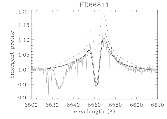
Figure 6: Clumped models for $\zeta$ Pup, compared to H_α(left) and the IR/radio continuum (right). The best-fitting model (cf. Table 6, first entry) is displayed in bold. Other curves: variation of the clumping factor in individual regions, by a factor of two; dotted: $f_{\rm cl}(1.12{\ldots}1.5$ $R_{\ast}$) 5.5$\rightarrow$11; dashed: $f_{\rm cl}(1.5{\ldots}2$ $R_{\ast}$) 3.1$\rightarrow$6.2; dashed-dotted: $f_{\rm cl}(2{\ldots}15$ $R_{\ast}$) 2$\rightarrow$4; dashed-dotted-dotted: $f_{\rm cl}(>15$ $R_{\ast}$) 1$\rightarrow$2. Note that H_α remains sensitive to all variations except for the last one. The mid-/far-IR, on the other hand, is sensitive “only” to variations in the range $2{\ldots}15$ $R_{\ast}$.

Table 6 and Fig. 6 (bold), on the other hand, display our best solution for a clumped model which consistently reproduces H_α and the complete IR/radio band in parallel. In the spirit as outlined above, the mass-loss rate has been chosen from the region with lowest clumping, which in this case is the radio domain. By setting $f_{\rm cl}^{\rm far}$ to unity then, the adopted mass-loss rate is the largest possible one and corresponds to the “homogeneous” radio mass-loss rate, ${\dot{M}}$= 8.5 $\cdot 10^{-6}\,{\rm M_{\odot}/yr}$, cf. Fig. 5, right panel. In this case, the H_α-forming region displays a typical clumping factor of 5.5 (from $r$ = 1.12 to 1.5) to 3.1 (from $r$ = 1.5 to 2), and $\beta$ has been adapted to 0.7 to provide a perfect H_α fit.

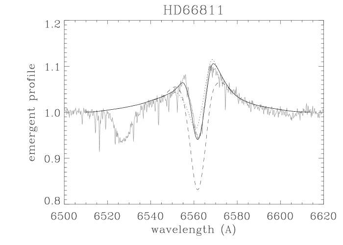
Figure 7: Clumped models for $\zeta$ Pup: influence of a different onset of clumping on H_α. Solid: best-fitting model, $r_{\rm in}=1.12$ $R_{\ast}$; dotted: $r_{\rm in}$ = $R_{\ast}$, i.e., clumping starting at the wind base; dashed: $r_{\rm in}=1.3$ $R_{\ast}$.

Fig. 7 displays the change in H_α when a different onset of clumping was chosen. If $r_{\rm in}$ were 1.3 (dashed profile), the central emission would be missing, whereas for $r_{\rm in}$ = 1.0 (dotted profile, corresponding to a model which is clumped from the wind base on), the absorption trough is not perfectly reproduced: the position of maximum depth is located at too high velocities, and the trough becomes too broad, resembling our best solution for the homogeneous model.

Table 6: Clumping factors, boundaries of different regions and mass-loss rates (in units of $10^{-6}{\rm M_{\odot}/yr}$) for three equally well fitting models of $\zeta$ Pup (strong wind, H_α in emission, $\beta=0.7$) and for our best fitting models of HD 209975 (moderate wind, H_α in absorption, $\beta=0.9$). The first solution for $\zeta$ Pup (which optimizes H_α) is displayed in the following figures, whereas the second one is almost indistinguishable from the first, though slightly worse in H_α, and slightly better in the mid-/far-IR and mm range. In the 3rd model it is assumed that helium remains doubly ionized everywhere. Note the large difference between the clumping properties of the two stars.

reg.	1	2		3	4/5		${\dot{M}}$	comment
HD 66811
$r/R_{\star}$	$<$ 1.12	$<$ 1.5	$<$ 2	$<$ 15	$>$ 15			best fit
$f_{\rm cl}$	1	5.5	3.1	2	1		8.5	for Hα
$r/R_{\star}$	$<$ 1.12	$<$ 2		$<$ 15	$<$ 50	$>$ 50		best fit for
$f_{\rm cl}$	1	5		1.5	1.4	1	8.5	far-IR/mm
$r/R_{\star}$	$<$ 1.12	$<$ 1.5	$<$ 2	$<$ 15	$>$ 15			Heiii
$f_{\rm cl}$	1	11.8	10	2	1		5.8	everywhere
HD 209975
$r/R_{\star}$	$<$ 1.05	$<$ 1.5	$<$ 2	$<$ 15	$>$ 15
$f_{\rm cl}$	1	1	1-2	1-1.5	1.3		1.2	identical
$r/R_{\star}$	1	$<$ 2		$<$ 10	$<$ 50	$>$ 50		fit quality
$f_{\rm cl}$	1	1		1-1.5	1-10	1.3	1.2

From our arguments given at the end of Sect. 3.4, it should be clear that in particular the latter solution is not unique, since an alternative model with all clumping factors multiplied by an arbitrary factor $f$, in parallel with a mass-loss rate reduced by a factor of $1/\sqrt{f}$, would result in an identical fit. If, on the other hand, the perfectly matched absorption trough for our model with $r_{\rm in}$ = 1.12 were actually due to a clumping-free lower wind base (and not coincidentally matched due to somewhat erroneous departure coefficients and/or the specific observational snapshot), such a scaling would no longer work (because of the presence of an unclumped region), and our solution would become “almost” unique, at least regarding the clumping properties of the inner wind.

The “almost” refers to the fact that a different distribution of the individual regions, combined with somewhat different clumping factors, gives fits of similar quality. The 2nd entry of Table 6 is such an example. In this case, we have combined the region between $r$ = 1.12 to 2 into one region, whereas we have split the outer region, beyond $r$ = 15, into two regions, with a border at $r$ = 50. To fit H_α (with a slightly worse quality than displayed in Fig. 6), the innermost clumping factors had to be reduced (from 5.5 and 3.1 to an average factor of 5.0), whereas, by adapting the clumping factors in the middle and outer part, the fit quality at 60 $\mu{\rm m}$ becomes perfect and the quality at 0.85/1.3 mm remains preserved Note, however, that the overall stratification of the clumping factors is rather similar.

Fig. 6 displays the advantage of fitting H_α and the IR/radio range in parallel. Although the primary formation region of H_α is below 2 $R_{\ast}$, it also remains sensitive to variations of the clumping factors in the intermediate wind, $r\la 15$, as can be seen from the reaction in the line wings if $f_{\rm cl}$ is doubled from 2 to 4 (dashed-dotted profile). Of course, a variation of the clumping factors in the inner regions (dotted and dashed) has even more impact. On the other hand, as displayed in the right panel of this figure, the IR/radio band reacts complementarily to variations beyond $r$ = 2, although only from the mid-IR on ($\lambda\ga 10$ $\mu{\rm m}$). Thus, a combined analysis is able to provide tight constraints on the largest possible mass-loss rate and to scan the complete stratification of $f_{\rm cl}(r)$ (at least differentially, i.e., modulo a constant factor) if the far-IR is well observed. Concerning the possible degeneracy of clumping factors and $\beta$, we refer the reader to Sect. 4.3.

Fig. 8, finally, displays the possible error if the helium ionization were different to that assumed here (cf. Sects. 3.2 and 3.3.) If helium were singly ionized throughout the complete wind (instead of recombining only at $v_{\rm rec}$ = 0.86), the synthetic 10 and 20 $\mu{\rm m}$ fluxes in particular would become too low; compensating for this effect by increasing clumping factors is not possible, because H_α would then no longer be fit. If, on the other hand, helium were to remain doubly ionized in the outermost region also, the radio/mm (and the far-IR fluxes) would become larger than observed; in this case, a reasonable fit is still possible, by lowering the mass-loss rate and increasing the inner clumping factors (with a factor roughly corresponding to $(\dot{M}_{\rm old}/\dot{M}_{\rm new})^{2}$). The parameters for such a model (which fits both H_α and the entire IR–radio range) is given in Table 6, 3rd entry. The rather large difference in the resulting (maximum) mass-loss rate (factor 0.7) and clumping factors is due to the fact that our model of $\zeta$ Pup has a helium content which is twice solar, $Y_{\rm He}$ = 0.2. For solar helium abundance, as is typical for most of the other objects of our sample, the corresponding factor would be 0.85, as outlined in Sect. 3.3. Note again, however, that it is rather improbable that helium is still doubly ionized in the radio-forming region. From the consistency of the mm and radio fluxes, it is also clear then that the Helium ionization must be similar in the mm and the radio forming region, in agreement with our predictions for $v_{\rm rec}$.

Figure 8: Clumped models for $\zeta$ Pup in the IR/radio band: influence of helium ionization. Solid: best fitting model, with Heiii as the major ion for $v<v_{\rm rec}=0.86$ (5.3 $R_{\ast}$), and Heii as the dominant ionization stage outside $v_{\rm rec}$; dashed-dotted: Heii as the major ion everywhere; dashed: Heiii as the major ion in the radio emitting domain.

HD 209975.

Table 6 and Fig. 9 display the results of our combined fit procedure for this star, which has a moderate wind density and H_α in absorption. Again, we have indicated the resulting profiles/fluxes when the derived clumping factors are varied by a factor of two in specific regions, to check for their sensitivity. Most interestingly, this object can be fitted with almost constant clumping factors throughout the wind, in stark contrast to the above example. Indeed, with slightly different ${\dot{M}}$ and $\beta$, an almost equally perfect fit is possible with all clumping factors being unity. If at all, the (homogenous) radio mass-loss rate is somewhat higher than the mass-loss rate derived from H_α, so that in this case $f_{\rm cl}^{\rm in}$ is set to unity.

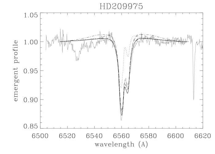
Figure 9: As Fig. 6, but for HD 209975. The best-fitting model (with all clumping factors at or close to unity) is displayed in bold. Other curves show the effects of varying, by a factor of 2, the clumping factors in individual regions alone. Dotted: $f_{\rm cl}(1.05{\ldots}1.5$ $R_{\ast}$) 1$\rightarrow$2; dashed: $f_{\rm cl}(1.5{\ldots}2$ $R_{\ast}$) 1$\rightarrow$2; dashed-dotted: $f_{\rm cl}(2{\ldots}15$ $R_{\ast}$) 1$\rightarrow$2; dashed-dotted-dotted: $f_{\rm cl}(>15$ $R_{\ast}$) 1.3$\rightarrow$2.6. Again, H_α remains sensitive to variations below $r$ = 15 $R_{\ast}$ (but see text), whereas the far-IR (not constrained by observations) is mostly sensitive to variations in the range 2…15 $R_{\ast}$. Note that the dashed solution is also consistent with the observations.

Note that a moderate clumping factor of 2 for $1.5<r<2$ is still consistent with the data, and that due to missing far-IR information (the indicated data denote upper limits derived by IRAS), the clumping in the intermediate wind remains somewhat unconstrained. After some experimentation, it turned out that the data are also consistent with a moderately clumped wind ($f_{\rm cl}=10$) in the region $10<r<50$, or a weakly clumped wind ($f_{\rm cl}=2$) in the region $3<r<50$ (not quoted in Table 6). Only for the outermost wind ($r>50$), do the clumping properties have to be similar to the inner wind conditions.

Since the innermost wind has the lowest clumping, no statement concerning its onset is possible within our approach. Thus, any scaled solution ($f_{\rm cl}$ multiplied with $f$, ${\dot{M}}$ reduced by $1/\sqrt{f}$) provides an equally perfect fit and cannot be excluded.

The second entry for HD 209975 in Table 6 refers to our “standard” division of the different regions used for winds with H_α in absorption, namely $r_{\rm mid}=2$ and $r_{\rm out}=10$. This scheme accounts for the fact that in moderate/low density winds the IR and radio emission is formed closer to the star. As can be seen from the best fitting clumping factors, the results do (almost) not depend on details of the specific borders.

In summary, the inner and outer wind of this object have similar clumping properties, whereas far-IR observations are required to constrain the intermediate region.

4.2 Clumping properties of the complete sample

Before discussing the results of our analysis for the complete sample, let us point out some general findings, and remind the reader that the derived clumping factors are independent of any uncertainty concerning radius and distance, since all our diagnostics (H_α/radio/IR) scale in an identical way with respect to these quantities, cf. Eq. 2 and corresponding discussion.

The core of H_α as a tracer of wind clumping below $r\approx 2R_{\star}$.

Our simulations show that the strength of the core of H_α, whether in emission or in absorption, is quite sensitive to the value of the clumping factor in the inner part of the wind, and thus can be used to determine this parameter out to distances of about $r\approx 2$. If one relies on the value of $\beta$ as derived by means of unclumped models, the corresponding (average) clumping factors are very precise, with an accuracy of roughly 10% (but see Sect. 4.3). Note particularly that clumping factors $f_{\rm cl}^{\rm in}$ of order 2 or larger are still visible for objects with H_α in absorption (see Fig. 9, dotted profile).

Constraints on the clumping factor beyond $r\approx 2R_{\star}$.

In addition to constraining the clumping properties in the lower wind, H_α can even serve as an indicator of wind clumping in layers beyond $r\approx 2$ (e.g, Fig.  6, left panel). How much beyond? The answer depends, of course, on the specific wind density, but some general statements for stars with H_α in emission are possible though. Usually, we found that reducing the extent of the intermediate clumped region 3 from $r_{\rm out}=15$ to about $r_{\rm out}=3$ has a noticeable effect on the strength of the H_α emission wings. The same is true if the boundary of region 2, $r_{\rm mid}=2$, is extended to a value of $r_{\rm mid}=3$. The effect becomes visible when the outer boundary moves from $r_{\rm out}=15$ to $r_{\rm out}=5$ and is insignificant if $r_{\rm out}$ is set to 8 stellar radii instead of $r_{\rm out}=15$.

For those objects with H_α in emission and missing far-IR/mm information, in Table 7, column 14, we have indicated the outermost radius, $r_{\rm out}^{\prime}$, to which H_α alone can provide information on the clumping factor, on the assumption that the region, $r_{\rm out}^{\prime}<r<r_{\rm far}$, is “unclumped” (or, more precisely, has the same clumping properties as region 5). In parallel, we also quote the corresponding value, $f_{\rm cl}^{\rm mid}$, which is somewhat larger than the original one (for $r_{\rm out}=15$), due to the reduced width of region 3. Indeed, for almost all objects, $r_{\rm out}^{\prime}$ is of the order of 5 $R_{\ast}$, except for HD 14947 and HD 192639, where H_α provides information only out to 3 $R_{\ast}$. Thus, it is safe to conclude that H_α constrains the clumping factor up to distances of $r=3{\ldots}5R_{\star}$ if in emission. Note, however, that in some cases, significant clumping in region 4 (from $r_{\rm out}$ to $r_{\rm far}$) has an effect on H_α, which leads to an additional constraint on the clumping in this region.

For objects with H_α in absorption, on the other hand, the intermediate region remains much less constrained (Fig. 9, left panel), and we will comment below on the corresponding limits.

Table 7: Clumping properties as derived from our combined H_α/IR/radio analysis. Stars are ordered according to H_α profile type (“pt”) and spectral type. Entries with name in bold are objects with extremely well-constrained clumping parameters.
$T_{\rm eff}$ is given in kK, and $\dot{M}_{\rm cl}$ is the largest possible mass-loss rate, in units of $10^{-6}{\rm M_{\odot}/yr}$. “ratio” gives the ratio of “clumped” mass-loss rate to optical results using unclumped models (cf. Table 1). $\beta_{\rm cl}$ is the velocity field exponent as derived or adopted here, $v_{\rm rec}$ and $r_{\rm rec}$ are the velocity (in units of $v_{\rm\infty}$) and radius where He recombines (see Sect. 3.2), respectively, and $r(\tau_{2})$ is the radius where the radio continuum becomes optically thick at 2 cm ($r_{\rm rec}$ and $r(\tau_{2})$ in units of $R_{\ast}$).
Clumping factors and boundaries are defined as in Sect. 3.4. For all models, region 1 with $f_{\rm cl}=1$ (not tabulated) extends from $r=1$ to $r_{\rm in}=1.05$, except for HD 66811 where $r_{\rm in}=1.12$, and $r_{\rm far}$ (defining the border between region 4 and 5) has been set to 50 $R_{\ast}$ always. For objects with H_α in emission or of intermediate type, and missing far-IR/mm data, $r_{\rm out}^{\prime}$ (with corresponding clumping factor) indicates the maximum radius to which H_α alone can provide constraints on the clumping, on the assumption that the outer wind is “unclumped” (see text). For objects with H_α in absorption, $f_{\rm max}^{\rm mid}$ gives the maximum possible clumping factor in region 3, which is still consistent with the data. $f_{\rm max}^{\rm out}$ is defined similar to $f_{\rm max}^{\rm mid}$, but for region 4. For comments on individual objects and corresponding fits, see Appendix B.

										region 2		region 3			region 4		reg. 5
Star	pt	$T_{\rm eff}$	${\dot{M}}$cl	ratio	$\beta_{\rm opt}$	$\beta_{\rm cl}$	$v_{\rm rec}$	$r_{\rm rec}$	$r(\tau_{2})$	$f_{\rm cl}^{\rm in}$	$r_{\rm mid}$	$f_{\rm cl}^{\rm mid}$	$f_{\rm cl}^{\rm mid}(r_{\rm out}^{\prime})$	$r_{\rm out}$	$f_{\rm cl}^{\rm out}$	$f_{\rm max}^{\rm out}$	$f_{\rm cl}^{\rm far}$
Cyg OB2#7	e	45.8	$\leq$4.0a,b	0.38	0.77	0.90	1.00	inf	29.7	5.0	2.0	4.0-6.0	7.0(5)	15	1.0	10.0	1.0
HD 190429A	e	39.2	9.5	0.59	0.95	0.95	0.85	6.2	49.6	3.0	2.0	3.0	3.5(5)	15	1.0	2.0	1.0
			7.5	0.46						5.0	2.0	5.0	5.8(5)	15	1.0	2.0	1.0
HD 15570	e	38.0	6.5	0.38	1.05	1.05	0.84	6.3	45.0	5.5	2.0	4.0-6.0		15	13.0	20.0	1.0
HD 66811	e	39.0	8.5	0.51	0.90	0.70	0.86	5.3	36.1	5.0	2.0	1.5		15	1.4	1.8	1.0
			4.2	0.51	0.90	0.70	0.86	5.0	36.5	5.0	2.0	1.5		15	1.4	1.8	1.0
HD 14947	e	37.5	10.0	0.59	0.95	0.95	0.81	5.0	37.9	3.1	2.0	2.5	4.0(3)	15	1.0	5.0	1.0
Cyg OB2#11	e	36.5	5.0	0.62	1.03	1.10	0.81	5.6	30.7	3.0	2.0	5.0	6.0(5)	15	1.0	15.0	1.0
HD 210839	e	36.0	3.0	0.38	1.00	1.00	0.83	5.9	24.7	6.5	4.0	10.0		15	1.0	8.0	1.0
HD 192639	e	35.0	$\leq$3.0a	0.48	0.90	1.14	0.82	6.3	27.7	3.5	2.0	3.5	6.0(3)	15	1.0	10.0	1.0
HD 30614	e	29.0	1.5	0.49	1.15	1.15	0.16	1.2	25.7	2.6	2.0	3.0	3.5(5)	15	1.0	4.0	1.0
Cyg OB2#8A	i	38.2	$\leq$8.0c	0.71	0.74	0.74	0.84	4.7	33.6	2.5	2.0	1.0-2.0	2.5(3)	10	1.0	10.0	1.0
Cyg OB2#10	i	29.7	2.74	1.00	1.05	1.05	0.17	1.2	23.2	1.4	2.0	1.8	2.0(3)	10	1.0	4.0	1.0
													$f_{\rm max}^{\rm mid}$
Cyg OB2#8C	a	41.8	$\leq$3.5d	0.82	0.85	1.00	0.94	17.3	33.0	1.0	2.0	1.0	-	10	1.0	5.0	1.0
HD 34656	a	34.7	3.0	1.15	1.09	1.00	0.60	2.5	28.2	1.0	2.0	1.0	-	10	1.0	8.0	6.0
HD 24912	a	35.0	$\leq$2.3a	0.94	0.80	0.90	0.85	6.1	16.4	2.1	2.0	5.0	7.0	10	1.0	2.0	1.0
			$\leq$1.2a	0.49						8.0	2.0	20.0	25.0	10	1.0	3.0	1.0
HD 203064	a	34.5	1.1	1.12	0.80	0.90	0.57	2.2	23.3	1.0	2.0	1.0	2.0	10	1.0	8.0	1.0
HD 36861	a	33.6	$\leq$0.4a	0.54	0.80	0.90	0.51	1.9	10.2	2.0	2.0	1.0	20.0	10	1.0	2.0	1.0
HD 207198	a	36.0	1.0	0.95	0.80	0.90	0.82	5.2	22.5	1.0	2.0	1.0	2.0	10	1.0	15.0	1.0
HD 37043	a	31.4	0.8	0.78	0.85	0.90	0.29	1.3	14.4	1.0	2.0	1.0	4.0	10	1.0	2.0	1.0
			0.25	0.24						12.0	1.3	1.0	20.0	10	1.0	10.0	1.0
HD 209975	a	32.0	1.2	1.08	0.80	0.90	0.42	1.6	27.1	1.0	2.0	1.0	1.5	10	1.0	10.0	1.3

^a) only upper limits of radio fluxes available; ${\dot{M}}$ maximum radio mass-loss rate.
^b) He assumed to be recombined in radio region (see Appendix B).
^c) upper limit, since non-thermal radio emitter; ${\dot{M}}$ from 2 cm flux.
^d) ${\dot{M}}$ from H_α, since radio fluxes (upper limits only) give larger value.

Table 7 summarizes the results of our simultaneous H_α/IR/radio analysis for the two objects already discussed in Sect. 4.1 and for the remaining ones. We have ordered the sample according to H_α profile type and spectral type. For almost all objects, we have used identical boundaries, $r_{\rm in}=1.05$, $r_{\rm mid}=2.0$ and $r_{\rm far}=50$, to obtain comparable results. The default values for $r_{\rm out}$ correspond to 15 (H_α in emission) and 10 (H_α in absorption or of intermediate type), but have been adapted where necessary. Detailed comments regarding the individual objects are given in Appendix B, where all fits are displayed as well.

Overall, our simulations show that for stars with H_α in emission, a simultaneous fit of the observed radio fluxes and the shape and strength of H_α, requires clumping factors which are always higher in the H_α-forming region than in the radio-forming one. For stars with H_α in absorption, the situation seems to be different: in most cases, the required clumping factors are of similar order in the inner and outer regions, as already discussed for the case of HD 209975. Note, however, that this preliminary impression is dependent on the actual value of $\beta$, a problem which will be discussed in our error analysis further below.

For all objects quoted with a definite mass-loss rate (and not only an upper limit), this value represents the largest possible value (for given $R_{\ast}$), usually derived from adopting an outer, unclumped wind with $f_{\rm cl}^{\rm far}=1$ or, for weaker winds, $f_{\rm cl}^{\rm out}$ = 1. These mass-loss rates correspond to the “usual” radio mass-loss rate. Only for one object, HD 34656, did the maximum mass-loss rate have to be derived from H_α, since the radio regime seems to be more strongly clumped than the lower wind, at least if the radio emission is purely thermal. Remember that the radio and H_α mass-loss rates for HD 209975 are consistent to within the error bars.

Because all our diagnostics depend on $\rho^{2}$, different solutions with lower mass-loss rates and scaled clumping factors are consistent with the observational data to a similar accuracy as obtained from our fits, except for the innermost cores of H_α (particularly if of P Cygni shape), due to our assumption of an unclumped innermost region. As already noted, these deviations remain very small for the derived values of $r_{\rm in}$ though.

For six objects, the maximum mass-loss rate could not be uniquely constrained, and the quoted limits correspond to the largest value consistent with the data. In five of theses cases (denoted by superscripts “a” and “d”), all radio fluxes are upper limits only, and consequently the derived mass-loss rates as well. One object (Cyg OB2#8A) is a confirmed non-thermal emitter (Bieging et al., 1989), and the adopted maximum mass-loss rate relies on the 2 cm which gives the lowest (radio) ${\dot{M}}$ within the available data set (see Sect. 2.1).

Of course, all objects with only upper limits for the radio flux(es) might be non-thermal emitters, and our interpretation depends on the assumption that the radio excess is due to thermal emission alone. In addition to these objects, three more stars (HD1̇90429A, HD 34656 and HD 37043 (SB2!)) have somewhat peculiar radio fluxes, and might also be non-thermal emitters.

Mostly because of these peculiarities (for more details, see Appendix B), we have given two possible solutions for HD 190429A, HD 37043 and also HD 24912 in Table 7, comprising a minimum and maximum solution with respect to the (relative) clumping properties. For HD 37043 and HD 24912, the 2nd entries are the more plausible ones (as discussed in the appendix), whereas for HD 190429A both solutions have similar problems (though the difference is not as large as for the other two stars).

Indicated by their name appearing in bold face, the remaining objects (six with H_α in emission, one with intermediate type and three with H_α in absorption) have well-constrained clumping properties, i.e., the derived results are robust if $\beta$ is not too different from the values derived or adopted here.

The latter quantity has been specified as follows. For objects with H_α in emission and of intermediate type, we have used the values from our unclumped analyses (see Tables 1 and 5) wherever possible, i.e., if satisfactory fits could be achieved. This turned out to be true in almost all cases, with the notable exception of $\zeta$ Pup, where our clumped analysis favours a much lower value ($\beta_{\rm cl}$ = 0.70) than previously found. For most objects with H_α in absorption (except Cyg OB2#8C and HD 34656, see Appendix B), because of missing constraints we used the “standard” value (from hydrodynamical models) of $\beta$ = 0.9, to obtain at least consistent results. Further consequences of this uncertainty are discussed in the next section.

For those stars where H_α is of P-Cygni shape or displays a well-refilled absorption trough, conclusive limits could be derived regarding the maximum value of $r_{\rm in}$, i.e., the maximum extent of a potentially unclumped region. In all cases, this region lies below 1.2 $R_{\ast}$.

In addition to the derived clumping factors which represent the best-fitting solution, we also provide maximum values for $f_{\rm cl}^{\rm mid}$ and $f_{\rm cl}^{\rm out}$ which are still consistent with our data and can be restricted further only by additional far-IR and sub-mm observations. For all objects with entries “above” Cyg OB2#8C in Table 7, $f_{\rm cl}^{\rm mid}$ could be constrained from the wings of H_α, either for the entirety of region 3 or, if indicated, at least out to $r_{\rm out}^{\prime}$. For the other objects, the wind density is too low to induce significant reactions in either H_α or the IR when the clumping properties in region 3 are changed, such that more definite statements are not possible.

Table 8: Upper and lower limits for the clumping factors in regions 2 and 3, corresponding to a variation of $\beta_{\rm cl}$ as indicated (“used” refers to the best fitting values tabulated in Table 7. For Cyg OB2#7, HD 15570 and Cyg OB2#8A we display the solutions for the larger values of $f_{\rm cl}^{\rm mid}$, which fit H_α but somewhat overestimate the 10 $\mu$m fluxes, see Appendix B). No entries are given for Cyg OB2#11 and HD 34656 due to the very unclear situation encountered for these objects (see Appendix B). Usually, the minimum value of $f_{\rm cl}$ refers to the maximum of $\beta_{\rm cl}$, and vice versa. For objects with an uncertainty in ${\dot{M}}$ being larger than typical, column 3 indicates the corresponding range (in units of $10^{-6}{\rm M_{\odot}/yr}$). For entries with purely negative $\Delta\dot{M}$, the correction refers to the maximum value of $\beta_{\rm cl}$; in these cases, the outer wind must also be clumped, with values as indicated by $f_{\rm cl}^{\rm far}$. For HD 209975, the positive correction refers to $\beta_{\rm cl}$ = 0.7 with $f_{\rm cl}^{\rm far}=1$, no correction but $f_{\rm cl}^{\rm far}=1.3$ refers to $\beta_{\rm cl}$ = 0.9, and the negative correction and $f_{\rm cl}^{\rm far}=3.5$ refers to $\beta_{\rm cl}$ = 1.1.

			$\beta_{\rm cl}$			$f_{\rm cl}^{\rm in}$			$f_{\rm cl}^{\rm mid}$
Star	${\dot{M}}$cl	$\Delta\dot{M}_{\rm cl}$	min	used	max	min	used	max	min	used	max	$f_{\rm cl}^{\rm far}(\beta_{\rm max})$
Cyg OB2#7	$\leq$ 4.0		0.80	0.90	1.10	3.1	5.0	7.0	5.5	6.0	7.0
HD 190429A	9.5		0.85	0.95	1.10	2.0	3.0	3.8	2.5	3.0	3.5
	7.5		0.85	0.95	1.10	3.2	5.0	6.5	4.5	5.0	6.5
HD 15570	6.5		0.85	1.05	1.15	3.8	5.5	7.5	4.5	6.0	7.5
HD 66811	8.5/4.2		0.60	0.70	0.90	3.0	5.0	6.0	1.5	1.5	2.0
HD 14947	10.0	+/-2.0	0.85	0.95	1.15	1.7	3.1	3.8	2.0	2.5	3.0
Cyg OB2#11	5.0	+/-0.5	1.00	1.10	1.40	1.8	3.0	4.0	3.5	5.0	5.3
HD 210839	3.0		0.80	1.00	1.10	5.0	6.5	8.0	5.0	10.0	12.0
HD 192639	$\leq$ 3.0		1.00	1.14	1.25	2.8	3.5	5.0	2.5	3.5	4.5
HD 30614	1.5		1.00	1.15	1.25	2.5	2.6	3.5	2.0	3.0	4.0
Cyg OB2#8A	$\leq$8.0		0.65	0.74	1.10	1.2	2.5	3.0	1.5	2.0	3.0
Cyg OB2#10	2.74		0.80	1.05	1.15	1.1	1.4	2.2	1.5	1.8	2.3
HD 24912	$\leq$ 2.3		0.70	0.90	1.10	1.0	2.1	6.0	1.0	5.0	7.0
	$\leq$ 1.2		0.70	0.90	1.10	3.0	8.0	20.0	1.0	20.0	25.0
HD 203064	1.1	-0.4	0.70	0.90	1.10	1.0	1.0	2.0	1.0	1.0	2.0	2.5
HD 36861	$\leq$ 0.4		0.70	0.90	1.10	1.0	2.0	15.0	1.0	1.0	20.0
HD 207198	1.0	-0.35	0.70	0.90	1.10	1.0	1.0	2.5	1.0	1.0	2.0	3.0
HD 37043	0.8	-0.3	0.70	0.90	1.10	1.0	1.0	3.0	1.0	1.0	4.0	2.6
	0.25		0.70	0.90	1.10	3.0	12.0	30.0	1.0	1.0	20.0
HD 209975	1.2	+0.1/-0.4	0.70	0.90	1.10	1.0	1.0	1.3	1.0	1.0	1.5	1.3/3.5

4.3 Errors in the derived clumping factors

In the following, we will concentrate on the errors introduced into the derived clumping factors; errors in the mass-loss and modified wind-momentum rates are dominated by errors in the angular diameter and radius, but do not affect the major outcome of our investigation.

Let us first mention that during our detailed fits we found no systematic problem concerning an underestimation of the $N$- and $Q$-band fluxes, so that at least our absolute flux calibration seems to be appropriate (see Sect. 2.4.1). On the contrary, for some objects ($Q$-band: HD 15570; $N$-band: Cyg OB2#11, #10 and HD 207198), these fluxes lie above our predictions for the best-fitting model. To investigate this point in more detail, however, additional fluxes in the mid- and far-IR are required.

Uncertainties introduced by the radio continuum.

To determine the uncertainty in the derived clumping factors due to uncertainties in the observations (e.g., intrinsic errors and/or temporal variability of the observed radio fluxes), we have varied $f_{\rm cl}^{\rm in}$ and $f_{\rm cl}^{\rm mid}$ by identical factors and adapted ${\dot{M}}$ accordingly, until the observed radio fluxes could no longer be matched. From these experiments, it turned out that the clumping factors in the regions traced by H_α (i.e., below $r=3{\ldots}5$) are accurate (on an absolute scale) to within 20 to 50%, whereas the ratio of the clumping factors in the various regions remains preserved. Remember that the derived clumping factors scale inversely with $\dot{M}^{2}\leavevmode\nobreak\ ({\rm radio})\propto F_{\nu}^{1.5}$, i.e., $\delta f_{\rm cl}/f_{\rm cl}\approx-1.5\,\delta F_{\nu}/F_{\nu}$. Extreme cases regarding this uncertainty in the radio fluxes are HD 190429A, HD 14947 and Cyg OB2#11 (cf. Table 8, 3rd column).

The degeneracy of $\beta$ and clumping factors in the inner wind.

As noted above, the strength of the core of H_α is highly sensitive to the value of the clumping factor in the inner part of the wind, below $r\approx 2R_{\star}$. It is also sensitive to the value of the velocity exponent, $\beta$, and in a similar way: larger values of both $\beta$ and clumping factors lead to more emission in the line core, giving rise to an unfortunate degeneracy. Note, however, that the well-known $\beta$ vs. ${\dot{M}}$ degeneracy (e.g., Puls et al. 1996) has “vanished”, since the (maximum) mass-loss rate is determined from the radio regime. Except for the weakest winds (which cannot be observed in the radio anyway), the radio fluxes remain unaffected by the shape of the velocity field (cf. Table 7, column 10).

This new degeneracy requires an investigation into the question of how far any uncertainty in $\beta$ will propagate into the errors of $f_{\rm cl}$. To this end, we have varied $\beta$ and determined the appropriate values of $f_{\rm cl}^{\rm in}$ and $f_{\rm cl}^{\rm mid}$ such that the quality of our H_α fit remained preserved. For profiles with H_α in emission and of intermediate type, the minimum and maximum values of $\beta$ were taken from those solutions which were still compliant with the observed profile shape. For objects with H_α in absorption, we used reasonable limits, at $\beta=0.7$ and $\beta=1.1$, respectively. Larger values could usually be excluded from the profile shape, whereas in certain cases a lower value (though being larger than the physical limit, $\beta\geq 0.5$) might still be possible. This procedure is somewhat similar to our approach to resolving the alternative $\beta$ vs. ${\dot{M}}$ degeneracy in homogeneous winds, when ${\dot{M}}$ is derived from H_α alone (cf. Paper I).

In Table 8 we have summarized the results of our simulations. As expected, for stars with H_α in emission, the uncertainty in $\beta$ is not dramatic. This uncertainty leads to an average uncertainty in $f_{\rm cl}^{\rm in}$ of about $\pm$ 30%, whereas for objects with H_α in absorption, much larger uncertainties are possible (factors of between 2 and 7), if $\beta$ were 0.7 instead of 0.9.

For most of the objects with H_α in absorption, a larger value of $\beta$ (1.1 instead of 0.9) would have some interesting consequences. Since for these objects the inner clumping factors are of the order of unity for $\beta=0.9$, an increase of $\beta$ cannot be compensated for by diminished clumping. Consequently, the mass-loss rate must be decreased in this case, to reduce the wind emission. Table 8, 3rd column, shows that the required amount is of the order of 30%. To still obtain a consistent fit in the radio domain, $f_{\rm cl}^{\rm far}$ has to become larger than unity, of the order of 2. Thus, if low-density winds were to have a velocity field exponent larger than the standard one, the differences to the objects with emission profiles would become even more pronounced: in this case, the outer region would be even more clumped than the inner one. Only if $\beta$ were close to its lower limit, would the clumping properties of some of the thin winds become similar to those of high-density winds.

Concerning the resulting uncertainties for $f_{\rm cl}^{\rm mid}$ (region 3), the situation for H_α emission type objects is similar as for $f_{\rm cl}^{\rm in}$. The average minima and maxima lie $\sim\pm\,20\%$ below and above the best-fitting value of $\beta$. For the objects with weaker winds, on the other hand, $f_{\rm cl}^{\rm mid}$ still remains unconstrained, and in all cases the upper limits as already quoted in Table 7 remain valid.

One last comment. Concerning our model(s) for $\xi$ Per (HD 24912), we note in Appendix B that large values for the clumping factors in region 3 ($f_{\rm cl}^{\rm mid}$) are required if the small emission humps bluewards and redwards of the H_α absorption trough are to be explained by clumping. If, on the other hand, $\beta$ were 0.7 for this object, these humps can be created from region 2 alone.

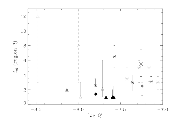
Figure 10: Clumping factors, $f_{\rm cl}^{\rm in}$ (region 2), for our sample (cf. Table 8), as a function of the distance-invariant quantity, $\log Q^{\prime}$ ($Q^{\prime}=\dot{M}/R_{\star}^{1.5}$, with ${\dot{M}}$ the largest possible mass-loss rate, in units of ${\rm M_{\odot}/yr}$ and $R_{\ast}$ in units of $R_{\odot}$). Remember that most clumping factors refer to outermost clumping factors set to unity. Asterisks: objects with H_α in emission; diamonds: objects with intermediate H_α profile type; triangles: objects with H_α in absorption. Black colors: objects with definite maximum mass-loss rates (corresponding to bold-face entries in Table 7). Grey colors: objects with upper limits for ${\dot{M}}$ and corresponding lower limits for $f_{\rm cl}^{\rm in}$. Maximum values of $f_{\rm cl}^{\rm in}$ correspond to minimum values of $\beta_{\rm cl}$, and vice versa for the minimum values. The open triangles with solid error bars display the high-${\dot{M}}$–weak-clumping solution for HD 24912 and HD 37043, and the open triangles with dashed error bars the alternative low-${\dot{M}}$–strong-clumping solution for these objects.

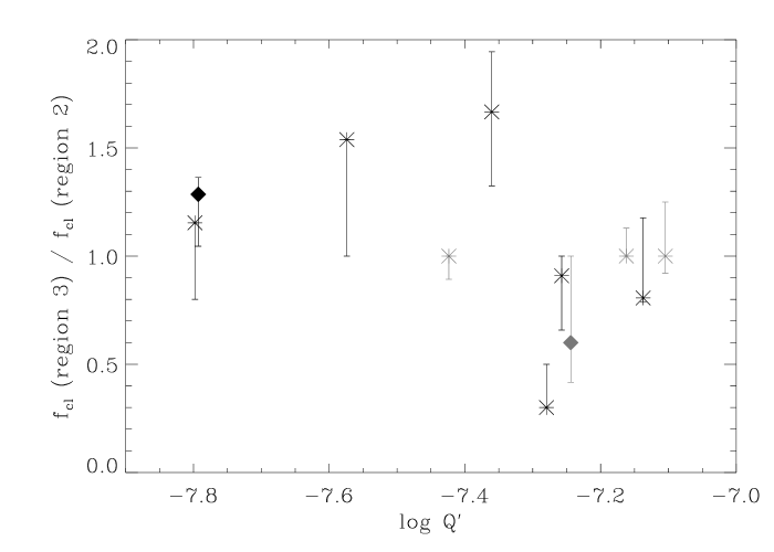
Figure 11: As Fig. 10, but for the ratio $f_{\rm cl}^{\rm mid}/f_{\rm cl}^{\rm in}$, and objects with H_α in emission or of intermediate profile type only. The star with the lowest ratio (0.3) is $\zeta$ Pup. For the three objects with a given interval for $f_{\rm cl}^{\rm mid}$ (Cyg OB2#7, HD 15570 and Cyg OB2#8A, see Table 7), we have used the mean value regarding this interval.

5 Discussion

5.1 Clumping properties as a function of wind density

Fig. 10 displays the derived clumping factors for region 2 (i.e., the first clumped region) as a function of $\log Q^{\prime}=\log\dot{M}/R_{\star}^{1.5}$, i.e., a quantity which is closely related to the mean wind density, but is additionally distance invariant. Remember that in the present context ${\dot{M}}$ is the largest possible mass-loss rate, and that most of the derived factors refer to outermost clumping factors set to unity. In other words, they have to be regarded as a measurement of the clumping properties of the inner wind relative to the outermost one. Details of the figure are given in the corresponding caption.

The most important conclusions which can be drawn from this figure are the following. For thinner winds with $\log Q^{\prime}\la-7.5$ (a regime which is populated by objects with H_α in absorption or of intermediate type, but also by the supergiant $\alpha$ Cam), the inner wind seems to be clumped by a similar degree as the outermost one, at least if we discard the alternative low-${\dot{M}}$–strong-clumping solutions for HD 24912 and HD 37043 (open triangles with dashed error bars). Note that if the latter solutions were the actual ones (and we have indicated that this is rather possible), then both stars are behaving completely different to the other absorption-type stars.

On the other hand, for stronger winds (almost all stars with emission profiles, plus Cyg OB2#8A), the inner wind seems to be more strongly clumped than the outermost one, with an average ratio of 4.1 $\pm$ 1.4. Of course, for this class of objects there is also the possibility that we encounter moderately ($f_{\rm cl}^{\rm in}\approx 3$) and stronger ($f_{\rm cl}^{\rm in}\approx 5$) clumped lower wind regions, or that the degree of clumping decreases again towards the largest wind densities. However, due to the restricted number of objects, the influence of temporal variations (Sect. 2.1) and the error introduced by the uncertainty of the continuum flux level, such statements cannot be verified at the present time.

Fig. 11 displays the ratio of clumping factors in the intermediate and inner part of the wind, for objects with H_α in emission or of intermediate type; for those objects, this ratio could be constrained in a rather robust way. In most cases, the clumping properties in both regions are either similar, or the (average) clumping factors increase moderately from region 2 towards region 3, at most by a factor of 2. Let us reiterate, however, that region 3 is rather extended (i.e., local values might deviate from their average ones), and that we cannot derive definite values for radii larger $r_{\rm out}^{\prime}\approx 5R_{\star}$, except for few cases, because H_α becomes insensitive in this region, and strong constraints from the IR continuum are missing. Future observations will help to clarify this situation.

For objects with H_α in absorption, at least upper limits for the clumping factors in region 3, $f_{\rm max}^{\rm mid}$, could be derived (see Tables 7 and 8). For three well-constrained objects, HD 203064, HD 207198 and HD 209975, these upper limits lie between 1.5 and 2, i.e., they might be twice as large as the corresponding values for $f_{\rm cl}^{\rm in}$, but are still rather low. For the remaining stars, the maximum values for $f_{\rm cl}^{\rm mid}$ lie in between 4 and 25, but only for HD 24912 is a large value actually needed, if the observed emission humps are to be interpreted in terms of clumping and $\beta$ were of order 0.9 or larger (see above).

Concerning the clumping properties in region 4 ($15\leq r\leq 50$), finally, definite statements are only possible for those 3 stars observed in the mm region (see below). For the rest, solutions with $f_{\rm cl}^{\rm out}=1$ are consistent with the observations, but larger values ($f_{\rm max}^{\rm out}$ = 2…20, cf. Table 7) are possible as well. For HD 190429A, HD 14947, HD 30614 and Cyg OB2#10, H_α still reacts to variations of the clumping factor in region 4, and $f_{\rm cl}^{\rm out}$ could be restricted to values from 2 to 4. Since for weaker winds the radio-forming region can extend into region 4, for a number of objects with H_α in absorption, $f_{\rm cl}^{\rm out}$ is better defined than for the rest, particularly for HD 24912 and HD 36861, with $f_{\rm cl}^{\rm out}\la 2{\ldots}3$.

Figure 12: Wind-momentum–luminosity relation for our sample. Modified wind-momentum rate, $D_{\rm mom}=\dot{M}v_{\infty}(R_{\star}/R_{\odot})^{0.5}$, in cgs units. Left panel: mass-loss rates derived from H_α, using homogeneous models, cf. Table 1. Right panel: largest possible mass-loss rates, from this investigation. Upper limits indicate those cases where radio fluxes are upper limits and/or non-thermal emission cannot be excluded. Asterisks: objects with H_α in emission; diamonds: objects with intermediate profile type; triangles: objects with H_α in absorption. Dashed line indicates theoretical prediction by Vink et al. (2000). “ZP” indicates the large and low distance solution for $\zeta$ Pup (see text). For the three objects at $\log L/L_{\odot}=5.3$ (HD 203064, HD 207198 and HD 209975), the lowermost solution indicates their position if the velocity exponent was larger than expected ($\beta=1.1$ instead of $\beta=0.9$). In this case, the (unclumped) H_α  mass-loss rate would be lower than the radio mass-loss rate, and the wind would have to be more strongly clumped in the radio regime than in the innermost region. For HD 37043, at $\log L/L_{\odot}=5.45$, the lowermost solution corresponds to the 2nd entry in Table 7.

The best-constrained objects within our sample are $\zeta$ Pup, HD 15570 and HD 210839, due to IRAS (for $\zeta$ Pup) and mm observations. The first of these objects, $\zeta$ Pup, displays the only notable exception concerning the ratio of $f_{\rm cl}^{\rm mid}$ and $f_{\rm cl}^{\rm in}$, namely that region 3 is much less clumped than region 2. In other words, maximum clumping must be close to 2 $R_{\ast}$, or even lower (cf. Fig. 6 and Table 6). For this star, the derived clumping factor for region 4 (extending from 15 to 50 $R_{\ast}$) is even lower than for region 3: at most, $f_{\rm cl}^{\rm out}\la 1.8$.

For HD 15570, on the other hand, regions 2 and 3 are similarly clumped, and the derived clumping factor might increase even further towards region 4, with $f_{\rm cl}^{\rm out}$ being 5 to 20 times larger than the average clumping in the radio-emitting region. In the unlikely case that the wind is not recombined at 1.3 mm, even $f_{\rm cl}^{\rm out}=1$ is possible. For this object, the mm measurements from scuba are extremely valuable, though the rather large error bars leave the situation not as clear as desirable.

For $\lambda$ Cep (HD 210839), finally, the intermediate region is more heavily clumped than the inner one, whereas region 4 could be constrained (again via scuba observations) to display clumping factors between 1 and 8. It remains to be clarified whether the two different observed flux levels (Tab. 4, Fig 14, 2nd row) are a sign of significant temporal variability of the outer wind (indicating a temporal variation of clumping or a non-negligible effect of macro-structures) or the “truth” lies in between both measurements, which are still consistent within the claimed error bars.

In summary, at least one of these three objects is rather weakly clumped in region 4. Although the same might be true for the other two stars (accounting for the lowest possible fluxes), a significantly clumped outer region is more probable.

5.2 Wind-momentum–luminosity relation

Before discussing some further implications of our findings, let us consider the wind-momentum–luminosity relation for our stellar sample, accounting for the results derived in the present paper. Fig. 12 displays two such relations, in comparison with the theoretical predictions by Vink et al. (2000). In the left panel, we show the results using H_α mass-loss rates derived by unclumped models, updated for a re-determined stellar radius (Sect. 2). As already noted in Paper I and outlined in the introduction, objects with H_α in absorption and of intermediate type are perfectly consistent with the predictions (except for a few objects at $\log L/L_{\odot}<5.35$; see below), whereas objects with H_α in emission populate a strip parallel to, but above, the predictions. Only the large-distance solution for $\zeta$ Pup lies on the relation, whereas the low-distance solution displays the same discrepancy as the other stars (both solutions indicated by “ZP”).

In the right panel, we display our new results, with mass-loss rates from Table 7. These mass-loss rates are the largest possible ones, and are essentially the radio mass-loss rates if the winds were unclumped in the radio-forming regime. Except for this assumption, the largest errors present in this figure are due to errors in the distance estimate. We have deferred from a rigorous error analysis concerning this problem, as this is beyond the scope of the present investigation.

What is obvious from this plot, however, is that the agreement between observations and theoretical predictions has significantly improved. Almost all objects now lie very close to the theoretical relation, independent of profile type.

The reason, of course, is that the newly derived (radio) mass-loss rates for emission-profile objects are smaller than the H_α mass-loss rates (see Table 7, column “ratio”), by an average factor of $0.49\pm 0.10$. Most interestingly, this is almost exactly the same factor which has been claimed in Paper I (0.48, drawn from a much larger sample), and which has been used a priori in our de-reddening procedure (see Sect. 2.6). A factor of the same order (0.42) has also been found by Fullerton et al. (2006), for a sample comprising objects similar to those considered here. For objects with H_α in absorption and of intermediate type, H_α and radio mass-loss rates agree well, and they remain at their “old” position. Note that for the only absorption-type object in the sample of Fullerton et al. with H_α and radio data available in parallel (HD 149757), a comparable agreement was found, supporting our results.

Due to the shift in wind-momentum rate, the new position of $\zeta$ Pup (larger distance) is completely inconsistent with the rest, whereas the conventional, lower-distance solution matches the predictions perfectly. The same problem was found in Paper I (after applying an average down-scaling of wind momenta, in anticipation of clumping effects), and our present result (which confirms this expectation) seems to favour a lower radius.

In accordance with our reasoning in Paper I, however, we like to point out that $\zeta$ Pup is a “bona fide” runaway star, (i.e., its parent association, Vela R2, has been identified by Sahu & Blaauw 1993). Based on Hipparcos data, Vanbeveren et al. (1998) argued that $\zeta$ Pup could have become a runaway as a result of a supernova explosion in a massive close binary, which might explain its peculiar characteristics, such as enhanced He and N abundances at the stellar surface, high peculiar and rotational velocities, and its overluminosity. The reason why the wind-momentum rate should be lower than for other objects remains to be clarified though.

Whereas the “new” WLR agrees extremely well with the theoretical predictions for objects with $\log L/L_{\odot}>5.35$, the three best-defined absorption-type stars at the lower luminosity end of our sample (HD 203064, HD 207198 and HD 209975) lie too high, by a factor of $\approx 2.5$. A similar effect was found in Paper I, though at the time it was not clear whether or not their winds are clumped in the H_α-forming region to a similar degree as emission type objects. In addition to wind momenta based on nominal radio mass-loss rates, we have also indicated (by the lower end of the displayed bars) their position if the velocity exponent were to be larger than expected ($\beta=1.1$ instead of $\beta=0.9$). In this case, the (unclumped) H_α  mass-loss rate would be lower than the radio mass-loss rate, and the wind would have to be more strongly clumped in the radio regime than in the innermost region (cf. Table 8). Even in this case, a discrepancy of a factor of $\approx 1.7$ would still be present. To unify these objects with the others by clumping arguments alone would require that they have to be much more clumped in the radio regime (on an absolute level).

Of course, one might argue that this problem is not related to (unknown) physics but to wrong distances and radii. Though this might be possible accounting for the mean errors in modified wind-momentum rate (0.13 dex) and luminosity (0.19 dex) derived for Galactic objects in Paper I, it is more plausible to invoke physical reasons, since we have to explain an identical problem for three different stars (with different $T_{\rm eff}$) at identical positions in the diagram.

Again, we stress that all displayed positions rely on the derived, largest possible mass-loss rates. If the radio regime were clumped, downward corrections become necessary. In this case, however, the displayed agreement would be pure coincidence.

5.3 Implications and conclusions

The results from the previous section have confirmed our earlier hypothesis that the “old” H_α mass-loss rates for objects with H_α in emission are contaminated by clumping, and that, compared to theoretical predictions, these mass-loss rates are overestimated by a factor of at least 2…3. Regarding the different behaviour of objects with emission and those with absorption profiles, however, we seem to have invoked a somewhat erroneous explanation (see our arguments recapitulated in Sect. 1).

Indeed, if objects with H_α in absorption were clumped in the lower-wind region, in a similar way to emission-type objects, we would have seen this: note that the presence of clumping with factors as low as $f_{\rm cl}^{\rm in}=2$ is clearly visible (cf. Fig. 9). It must be stressed, however, that our present sample consists of supergiants and giants only, and that dwarfs (with a very low wind emission inside the core of H_α) are missing. At least for the latter luminosity class, our old arguments might still be valid. For example, if the wind base was actually unclumped (as allowed for by our analysis, but in contrast to the findings by Bouret et al. 2005), and H_α predominantly forms in this region, we would not see the clumping effects, though they would be present in, e.g., the mid-/far-IR.

Assuming for the moment that, on an absolute scale, the outer clumping properties are independent of wind density, our results imply that the different degree of consistency between the theoretical and observed WLR is likely related to a physical effect: inside the H_α-forming region, denser winds are more strongly clumped than (most of) the weaker winds, at least if $\beta$ is of the order of 0.9 or larger in the weaker winds (see Fig. 10).

What might be the origin of such a difference? Objects with H_α in emission have a large wind density and are usually supergiants with low gravity and a considerable Eddington-$\Gamma$. Thus, it is rather possible that they are subject to photospheric instabilities and/or pulsations, triggering a somewhat larger structure formation in the lower wind, compared to lower density winds from higher gravity objects. Indications of such a dependence are consistent with investigations regarding photospheric line-profile variability (increasing with stellar radius and luminosity), as outlined by Fullerton et al. (1996).

On the other hand, our findings are in some contrast to hydrodynamical simulations, at least regarding self-excited structure formation. If there was any dependence on wind density predicted at all, thin winds should be more strongly clumped than thick winds, because of the missing stabilization due to the continuum (Owocki & Puls, 1999), which induces a more heavily structured wind in the lower part. Note also, that in thin winds, (transonic) velocity curvature terms become important, leading to gradient terms in the source functions and modification of the line acceleration (Puls et al., 1998). Simulations by Owocki & Puls (1999) accounting for this effect resulted in a highly structured wind, with a moderately reduced mass-loss rate and a rather steep velocity law in the lower region. Thus, even the possibility that $\beta$ is low (which would increase the derived, lower clumping factors, cf. Table 8) cannot be completely excluded, although in this case, $f_{\rm cl}^{\rm in}\la 2$ (for the three well-defined objects) is still rather low.

Let us now compare our results with the predicted radial stratification of $f_{\rm cl}$ itself (Runacres & Owocki, 2002, 2005). As is true for our results, theory also depends on a number of assumptions. Most important in this context are:-

• the dimensionality of the hydrodynamical treatment, which is mostly 1-D (because of the complexity of calculating the radiative line force). First results from a 2-D approach (Dessart & Owocki, 2003) might indicate somewhat lower (factor of 2) clumping factors than those resulting from a 1-D treatment.

• the excitation of the line-driven instability. Almost all models investigated with respect to the clumping factor refer to self-excited perturbations. Unfortunately, externally triggered perturbations, such as sound waves and photospheric turbulence (see Feldmeier et al. 1997), and photospheric pulsations, have not been examined with regard to this quantity.

• the so-called line-strength cut-off, $\kappa_{\rm max}$. In order to keep the problem numerically treatable (i.e., to avoid too fine a grid resolution), Owocki et al. (1988) introduced an opacity cut-off regarding the driving lines, which is typically three dex below the actual value. Experiments performed by Runacres & Owocki (2002) showed that the clumping factor in the outer wind (around 50 $R_{\ast}$), in particular, can increase if more realistic values are used. The inner and outermost part seem to remain rather insensitive, at least if very low values for $\kappa_{\rm max}$ are avoided.

Thus, the numbers which will be quoted in the following might be considered in a qualitative sense, especially since, for our comparison, we have to estimate appropriate spatial averages over the different regions. In our approach, we have used clumping factors assumed to be spatially constant within certain regions, whereas Runacres & Owocki (2002) display the clumping factor as a function of $r$. The most decisive quantity regarding radiative transfer is the optical depth, being proportional to the spatial integral over $f_{\rm cl}(r)\rho(r)^{2}$ (assuming the source function to be unaffected by clumping), so that a meaningful comparison requires the predicted clumping factors, $f_{\rm cl}(r)$, to be averaged over $\rho^{2}$ inside the regions considered. To this end, we have used the results displayed in the various figures provided by Runacres & Owocki.

Table 9: Clumping factors as predicted by hydrodynamical simulations from Runacres & Owocki (2002), for the different regions as used in this investigation. The first average is a straight one, the 2nd is weighted with $\rho^{2}$ (see text). Note that these numbers are only approximate ones, since they have been derived from figures and not from tables.

region	$f_{\rm cl}$	$\langle f_{\rm cl}\rangle_{1}$	$\langle f_{\rm cl}\rangle_{2}$
1	1	1	1
2	1…4	2.5	$\ga$2.1
3	4…13	8.5	$\ga$4.7
4a	13…5	9	$\la$11.6
5a	5 …4	4.5	$\la$4.7
4b	13…20	16	$\ga$14
5b	20…4	12	$\la$15

^a $\kappa_{\rm max}$ from Owocki et al. (1988); ^b $\kappa_{\rm max}$ larger by a factor of 10.

Table 9 summarizes the predictions. Region 1 (the inner, unclumped region) typically extends to 1.3 $R_{\ast}$ (for thin winds, it might be narrower; see above), which is fairly consistent with the derived maximum extent of such a potentially unclumped domain ($r_{\rm in}\la$ 1.1…1.2 $R_{\ast}$).

Regarding the other regions, we have to discriminate between absolute numbers and numbers referring to the average clumping factor in region 5, which is of the order of 4…5 or even larger, if $\kappa_{\rm max}$ is increased beyond its “standard” value. Such large averages depend on results indicating that the outermost wind (beyond 1000 $R_{\ast}$) is also considerably clumped; cf. Runacres & Owocki (2005). Only for rather low values of $\kappa_{\rm max}$ is a smooth radio regime predicted.

For region 2, we find average values $f_{\rm cl}^{\rm in}\approx 2{\ldots}3$ (lower than in region 5!), for region 3 values around 4…5, and for region 4 values around 11, which again might be even larger for large $\kappa_{\rm max}$. Note that for different wind densities and wavelengths, the calculated averages for regions 3 and 4 might be higher and lower, respectively, than the indicated ones, depending on the radial position at which $\tau=1$ is reached. Finally, the predicted maximum is located at the border between regions 3 and 4 (around 15 $R_{\ast}$), but might be shifted towards larger radii for larger $\kappa_{\rm max}$.

Compared to our results, these predictions are significantly different, at least if the average clumping factor in the radio domain is of the order of 4 or larger. In this case, all H_α mass-loss rates should be lower than the radio mass-loss rates, which is definitely not true. Thus, either the clumping factors in region 2 are predicted as too low, or those in region 5 as too large!

Disregarding this problem, the average clumping factor should increase monotonically from region 2 to 4 according to theory, and at least some of our emission type objects (e.g., HD 15570) are compatible with this result (though for others $f_{\rm cl}^{\rm out}$ is of the same order or even lower than $f_{\rm cl}^{\rm mid}$). Only concerning the differential behaviour of region 2 to region 3, do most objects behave as predicted (Fig. 11). As outlined already above, the notable exception to this rule is $\zeta$ Pup, where the complete run of $f_{\rm cl}(r)$ and the position of its maximum definitely deviate from the predictions (and from the other objects investigated). Such a deviation was already found by Puls et al. (1993b), who tried to simulate the observed H_α profile and IR continuum for $\zeta$ Pup, based on hydrodynamical models from S. Owocki. Though they were quite successful in fitting H_α with a mass-loss rate just a factor of 2 lower than when using homogeneous models (and consistent with present estimates), the IR continuum was too strong at this ${\dot{M}}$, indicating lower clumping factors than predicted in region 3.

The real question, of course, concerns the absolute value of the clumping factors, and their dependence on stellar parameters. What has been derived in this investigation is the behaviour of the inner clumping properties relative to the outermost ones. To reiterate, if the outer clumping properties were independent of wind density and/or stellar parameters, thinner winds would be less clumped in the inner region than stronger winds, and we have indicated above a possible reason for this. If, on the other hand, the (absolute) clumping factors in the inner part were to be equal or even larger in thinner winds than in denser ones, we would meet a number of other problems requiring explanation. In this case:-

• the outer region of thinner winds has to be more clumped than in thicker winds.

• the consistency with the theoretical WLR would completely vanish.

• the WLR would again show a strong dependence on luminosity class and/or H_α profile type (even if the theoretically predicted off-set was wrong). Such a dependence is presently not understandable, since the major prediction of radiation-driven wind theory is that the modified wind-momentum rate should be dependent on luminosity alone (at least if the slope of the corresponding line-strength distribution function is not too different from its presently derived value).

The only way to clarify this situation is the inclusion of processes which do not depend on $\rho^{2}$. One such diagnostic is Pv (Massa et al., 2003; Fullerton et al., 2004, 2006) which under favourable circumstances scales $\propto\rho$ alone. The major problem here arises from the uncertainties regarding the ionization fraction of this ion, which might be additionally contaminated by the UV-tail of the X-ray emission. Assuming that Pv is a major ion between O4 and O7, Fullerton et al. (2006) derived a median reduction in ${\dot{M}}$ (compared to homogenous H_α and radio diagnostics) by a factor of 20, where thin winds seemed to be more affected than thicker ones. Note that this would imply clumping factors of the order of 100 in the radio regime!

Detailed NLTE investigations accounting for clumping, on the other hand, are only in their infancy, and again, the inclusion of X-ray effects is a difficult task. The only object within our sample which can be compared with such an investigation is HD 190429A, analyzed by Bouret et al. (2005). In their conclusions, they quote a reduction of a factor of three in ${\dot{M}}$, compared to a homogeneous mass-loss rate of 6 $\cdot 10^{-6}\,{\rm M_{\odot}/yr}$ derived from the far-UV, exploiting $\rho$- and $\rho^{2}$-dependent processes in parallel, and accounting for a consistent ionization equilibrium.

The derived homogeneous UV mass-loss rate is much lower than our homogeneous H_α value (radius and distance are comparable), and they speculate on strong variations in H_α, referring also to Scuderi et al. (1998), who report an increase of the H_α equivalent width between 1988 and 1991, by a factor of 2 (but see also Markova et al. 2005, who found no indications of such large changes in H_α, at least over an interval of one year between 1997 and 1998). Though the implied clumping factor (from a comparison of homogeneous and clumped UV mass-loss rates) would be not too different from “our” value, on an absolute scale there are much larger differences. Comparing their final mass-loss rate (1.8 $\cdot 10^{-6}\,{\rm M_{\odot}/yr}$, with $R_{\ast}$ = 19.5 $R_{\odot}$ and $v_{\rm\infty}$ = 2300 km s^-1) with our radio mass-loss rate (7.5…9.5 $\cdot 10^{-6}\,{\rm M_{\odot}/yr}$, with $R_{\ast}$ = 22.7 $R_{\odot}$ and $v_{\rm\infty}$ = 2400 km s^-1), this would suggest a strongly clumped radio regime, with $f_{\rm cl}^{\rm far}\approx 10{\ldots}16$, at least if there have been no major changes in the average wind properties between their UV and our radio observations. Additionally, Bouret et al. (2005) point to the fact that the predictions by Lenorzer et al. (2004) concerning Br_α indicate that the outer winds “would be less affected by clumping”, compared to the regions they could access. Thus far, the situation remains unclear.

Notably, the other object investigated by Bouret et al. (2005) is an object with H_α in absorption, and for this object they find a reduction in ${\dot{M}}$ by a factor of 7 (again with respect to UV observations alone). This result would agree with our statement from above that thin winds are expected to be more strongly structured than thick winds, at least if the latter are not externally triggered by photospheric disturbances.

Accounting for these findings and other investigations with similar results (e.g., Hillier et al. 2003; Bouret et al. 2003), there seems to be increasing evidence that the agreement between the theoretical and observed WLR (which, if real, would imply a smooth wind in the radio regime) is indeed just coincidence, and that the radio regime must be strongly clumped, maybe even more strongly than presently described by hydrodynamics.

Aside from the major implications such a reduction of mass-loss rates would have, e.g., regarding stellar evolution in the upper HRD and feedback from massive stars, such a result would also lead to the following problem: since the present theoretical WLR originates from consistent calculations of the radiative line force, lower wind momenta would imply that too much radiative pressure is available. A reduction of this quantity, however, is rather difficult (but see below).

Finally, let us note that a significant down-scaling of mass-loss rates would unfortunately also affect stellar parameters (again!). For the $\rho^{2}$-dependent results derived here, such scaling is easily possible, without modifying any result. Photospheric lines, on the other hand, might be differently affected by a strongly clumped, but weaker wind, since they do not always scale with $Q$, but depend on other combinations of ${\dot{M}}$, $R_{\ast}$ and $v_{\rm\infty}$ as well.

6 Summary and future work

In this investigation, we have performed a simultaneous analysis of H_α, IR, mm (if present) and radio data to constrain the radial stratification of the clumping factor in a sample of 19 O-type supergiants/giants, with dense and moderate winds (H_α in emission and absorption). All analysis tools used involve certain approximations, but we have ensured that the derived results comply with state-of-the art NLTE model atmospheres, by comparing and calibrating to a large grid of such models. Clumping has been included in the conventional approach, by manipulating all $\rho^{2}$-dependent opacities and assuming the inter-clump matter to be void. Caveats have been given to this assumption and other problems inherent to this approach, namely the neglect of disturbances of the velocity field due to the clumps, and the assumption of small length scales, related to the problem of porosity.

Instead of adapting the clumping-factor at each radial grid point (which is possible only if using optimization methods, requiring a well-sampled observed wavelength grid), we have introduced 5 different regions, with constant clumping factors inside each region. Because all our diagnostics depends on $\rho^{2}$ (except for the small contribution by electron scattering), the most severe restriction within our approach is given by the fact that we cannot derive absolute clumping factors, but only factors normalized to a certain minimum. Since in all but one case (HD 34656) this minimum was found to be located in region 5 (or, in other words, since in all those cases the radio mass-loss rate is the lowest), our normalization refers to the radio regime, and the corresponding (radio) mass-loss rate as derived here is the largest possible one. Other solutions are possible as well, with all clumping factors multiplied by a constant factor, $f$, and a mass-loss rate reduced by $\sqrt{f}$.

Our analysis is based on H_α line profiles, near-/mid-/far-IR fluxes taken from our own observations and the literature (de-reddened as detailed in Sect. 2.6), mm fluxes observed by scuba/sest (own and literature data), and radio data taken from our own VLA observations and the literature. We have discussed the issue of non-simultaneous observations: based on present-day observational facts, the H_α, IR and radio variability of thermal emitters is low enough so as not to pose any problems for our study, at least if the derived results are considered in a statistical sense. Within our sample, there is only one confirmed non-thermal emitter (Cyg OB2#8A), and three more objects display somewhat peculiar radio fluxes (HD 190429A, HD 34656, see above, and HD 37043). These objects might be non-thermal emitters as well, but this has to be confirmed by future observations. In any case, the derived mass-loss rates (from the minimum radio flux) can be considered as an upper limit.

As it turns out, the core of H_α provides very useful diagnostics for the clumping properties in the inner wind ($r\la 2R_{\star}$), and, if in emission, the wings can be used to constrain the clumping inside the first five stellar radii, with an additional check provided by IR data. If mm fluxes were available, the outer wind ($15R_{\star}\la r\la 50R_{\star}$) could be constrained as well. Only the region between $5R_{\star}\la r\la 15R_{\star}$ remains “terra incognita” in most cases, due to missing far-IR fluxes.

For ten stars in our sample (six with H_α in emission, one of intermediate type and three with H_α in absorption), the derived clumping factors are robust and lie within well-constrained error bars. For six stars (including Cyg OB2#8A), only upper limits for the radio mass-loss rate are available, and the derived clumping factors have to be considered as lower limits. Obvious differences to the best-constrained objects were not found though, except for HD 24912, which behaves atypically. The three remaining objects constitute HD 34656, which is the only object in our sample with an H_α mass-loss rate lower than the radio mass-loss rate (and as such has been discarded from our further analysis), HD 37043, which exhibits similar problems to HD 24912 (but has a better-constrained radio mass-loss rate), and HD 190429A, which displays a certain degree of radio-variability. Taking the various results together, we can summarize our findings as follows:-

• for almost all objects (except for 3 stars with H_α in absorption and $\log L<5.35\,L_{\odot}$), the derived (radio) mass-loss rates are in very good agreement with the predicted wind-momentum–luminosity relation (Vink et al., 2000), in contrast to previous results relying on unclumped H_α data alone. If $\zeta$ Pup is located at the “close” distance, then it behaves as the rest. If, on the other hand, it is located further away, its (radio) wind-momentum rate would lie considerably below the predictions.

• the mean ratio of radio mass-loss rates to unclumped H_α mass-loss rates for stars with H_α in emission is 0.49 $\pm$ 0.10. This is almost exactly the same factor as found in Paper I, by shifting the observed WLR (using unclumped models) for these objects onto the predicted one. It also agrees well with recent findings from Fullerton et al. (2006).

• the average, normalized clumping factor in the innermost region ($r\la 2R_{\star}$) of stars with H_α in emission is $\sim 4.1\pm 1.4$.

• thinner winds with H_α in absorption have lower normalized clumping factors in this region. For all three stars with robust constraints, these factors are similar to those in the radio region, at least if the velocity exponent is not too different from the hydrodynamical prediction, $\beta\approx 0.9$. Factors of the order of $f_{\rm cl}^{\rm in}\ga 2$ can be excluded, due to the sensitive reaction of H_α.

• for all objects where H_α is of P Cygni shape, or displays a well-refilled absorption trough, the maximum extent of a potentially unclumped region can be limited to lie inside $r\la 1.2R_{\star}$.

• in most cases, the clumping factors in the inner and adjacent region ($2R_{\star}\la r\la 5{\ldots}15R_{\star}$) are comparable or increase moderately from inside to outside. Only for $\zeta$ Pup, does our analysis restrict the maximum clumping at $r\la 2R_{\star}$.

• the presence of clumping introduces a new degeneracy in the results, namely between the velocity field exponent, $\beta$, and the clumping factors. If $\beta$ is lower than assumed or derived from the fits, the clumping factors are larger, and vice versa. Extreme deviations of $\beta$ from values obtained from an unclumped analysis can be excluded though. Interestingly, a perfect fit for $\zeta$ Pup requires $\beta=0.7$, contrasted with $\beta=0.9$ from unclumped diagnostics (Repolust et al., 2004).

• two of the three stars with mm-observations (HD 15570 and HD 210839) indicate a certain probability that the outer region 4 ($15R_{\star}\la r\la 50R_{\star}$) is considerably more clumped than the radio domain (but remember the rather large error bars on the mm data), whereas the third star, $\zeta$ Pup (with negligible observational errors), displays similar clumping properties in both regions.

• Our results differ from hydrodynamical predictions (incorporating the intrinsic, self-excited line-driven instability, Runacres & Owocki 2002, 2005) at least in one respect: the latter imply a larger radio than H_α mass-loss rate (or, alternatively, lower clumping in the inner than the outer wind), which is definitely not true for our sample.

In addition to the conclusion that one of the best-observed massive stars, $\zeta$ Pup, might be a rather atypical representative of its kind (maybe due to its possible expulsion from a close binary system), the major implications of these findings can be stated within three different assumptions concerning the clumping properties of the outermost regions:-

• The radio region is not, or only weakly, clumped.
  In this case, our “old” hypothesis (concerning a shift of mass-loss rates for objects with H_α in emission, due to clumping) would be confirmed, but there would be a physical difference between denser and thinner winds, in the sense that thinner winds would be less clumped than thicker winds in the inner region. This difference might then be related to different excitation mechanisms of structure formation. If assumption (a) were true, the theoretical WLR would be perfectly matched. On the other hand, the absolute numbers for clumping factors and mass-loss rates would be in severe contrast to results from other investigations that have used alternative diagnostics, not directly affected by clumping (e.g., the Pv resonance lines).

• The radio region is strongly clumped, but the outermost clumping factors are independent of wind density.
  In this case, a unification with results from other diagnostics is possible, and the present mass-loss rates would have to be significantly revised, with serious implications for the evolution of, and feedback from, massive stars. Again, weaker winds would be less clumped in the inner region, and the theoretical WLR would no longer be matched. One of the most robust predictions from radiation-driven wind theory, namely that the modified wind-momentum rate should depend almost exclusively on luminosity (and not on mass or gravity), would still be consistent with our data, even if there were an offset between the theoretical and observed WLR.

• The radio region is strongly clumped, but the degree of clumping is different for different wind densities.
  This case is also consistent with present data, but would again imply, in addition to different offsets between the theoretical and observed WLR, that the observed WLR is dependent on a second parameter.

Obviously, the implications of all three assumptions pose their individual problems, and would have different consequences regarding the urgent question about the “true” mass-loss rates of massive stars. Since there is no direct way to measure the clumping in the radio regime, for further progress we suggest the following steps.

On the observational side, we have to: ($i$) re-observe some problematic objects at radio frequencies, to check their variability and to obtain further clues as to whether their emission is of thermal or non-thermal origin; and ($ii$) most importantly, accumulate far-IR and mm observations, to constrain the (normalized) clumping factor in the intermediate wind.

Once a reliable, normalized stratification has been obtained, it can be used as an input into state-of-the-art model atmosphere codes allowing for the inclusion of clumping and X-ray emission, with the mass-loss rate/velocity field adapted until all diagnostics (including the FUV/UV) are reproduced. This would also clarify the question concerning the ionization fraction of Pv. After having analyzed a significant number of objects, covering a large parameter space, we should be able to determine the importance of clumping, how it varies with spectral type and wind density, and what the actual mass-loss rates are.

Additionally, the derived clumping factors have to be incorporated into stationary wind-dynamics models. Using such models, we can investigate how far the corresponding wind properties differ from models without clumping, and check whether they are consistent with those derived from our observational diagnostics. Remember that if assumption (b) or (c) were true, the presently predicted line acceleration is much too large. It has to be clarified whether strong clumping is able to induce such a large shift in the ionization balance (see Sect. 3.4) that the bulk of the accelerating lines are shifted away from the flux maximum, such that a reduction in the acceleration is possible.

Finally, time-dependent hydrodynamic simulations must also continue. In particular, differences between self-excited and triggered structure formation have to be investigated, and conditions found which might allow for a much more strongly clumped radio domain than presently predicted (implied if assumptions (b) or (c) were true).

In this context, the following, concluding remark is relevant. Though the usual interpretation of clumping relies on a relation to the intrinsic instability of radiative line-driving, the issue of whether the redistribution of wind material occurs predominantly on small ($\sim$0.01 R_⋆) or large ($\sim$1 R_⋆) spatial scales has not yet been resolved. Small-scale clumping is suggested by observations of emission-line micro-variability in one of our targets (HD 66811; see Eversberg et al. 1998). However, structuring of hot-star winds on large scales is indicated by the ubiquitous presence of recurrent wind profile variability in the form of discrete absorption components (DACs; see, e.g., Prinja & Howarth 1986; Kaper et al. 1996). Since there is no consensus on the physical origin of DACs, the structure responsible for them is not included in the present generation of models.

Future studies will help to address this issue by determining whether objects with particularly well-studied DACs (e.g., HD 24912, HD 203064, HD 210839) can be modeled successfully without including large-scale structure. The presence of unexplained residuals from our self-consistent models (which cannot be discounted, due to missing far-IR observations, and which might already have been identified in the mid-IR fluxes of HD 24912, or in the somewhat discordant mm-observations of HD 210839, cf. Appendix B) with small-scale clumping would imply that large-scale structures also play a role in the redistribution of wind material, and would help to address the issue of whether DACs represent localized enhancements in the mass flux.

Appendix A The journal of the VLA observations

is given in Table 10 (see Sect. 2.3).

Table 10: Journal of the VLA observations, including observation dates, observing frequencies, time on targets, calibrators for flux-density bootstrapping and VLA configuration.

Star	date	freq.	time	cal	conf.
		(GHz)	(min)
Cyg OB2#7	Feb 15, 2004	4.86	60	3C286,3C48	CnB
Cyg OB2#7	Feb 15, 2004	8.46	45	3C286,3C48	CnB
Cyg OB2#10	Feb 15, 2004	4.86	20	3C286,3C48	CnB
Cyg OB2#10	Feb 20, 2004	4.86	40	3C286,3C48	C
Cyg OB2#10	Feb 15, 2004	8.46	20	3C286,3C48	CnB
Cyg OB2#10	Feb 20, 2004	8.46	25	3C286,3C48	C
Cyg OB2#10	Feb 15, 2004	14.94	20	3C286,3C48	CnB
Cyg OB2#10	Feb 20, 2004	14.94	40	3C286,3C48	C
Cyg OB2#11	Feb 15, 2004	4.86	30	3C286,3C48	CnB
Cyg OB2#11	Feb 15, 2004	8.46	30	3C286,3C48	CnB
Cyg OB2#11	Feb 15, 2004	14.94	30	3C286,3C48	CnB
HD 14947	Apr 04, 2004	4.86	30	3C48	C
HD 14947	Apr 04, 2004	8.46	30	3C48	C
HD 14947	Apr 04, 2004	14.94	30	3C48	C
HD 24912	Mar 09, 2004	4.86	20	3C286	C
HD 24912	Mar 09, 2004	8.46	15	3C286	C
HD 24912	Mar 09, 2004	14.94	20	3C286	C
HD 24912	Mar 09, 2004	43.34	20	3C286	C
HD 34656	Apr 04, 2004	4.86	40	3C48	C
HD 34656	Feb 09, 2004	8.46	45	3C147,3C48	CnB
HD 34656	Mar 09, 2004	14.94	20	3C286	C
HD 34656	Apr 04, 2004	14.94	20	3C147,3C48	C
HD 36861	Feb 09, 2004	8.46	40	3C147,3C48	CnB
HD 36861	Feb 09, 2004	4.86	40	3C147,3C48	CnB
HD 37043	Mar 09, 2004	4.86	30	3C286	C
HD 37043	Mar 09, 2004	8.46	30	3C286	C
HD 37043	Mar 09, 2004	14.94	30	3C286	C
HD 190429A	Mar 01, 2004	4.86	20	3C48	C
HD 190429A	Mar 01, 2004	8.46	20	3C48	C
HD 190429A	Mar 01, 2004	14.94	20	3C48	C
HD 190429A	Feb 26, 2004	43.34	20	3C48	C
HD 203064	Mar 01, 2004	4.86	60	3C48	C
HD 203064	Mar 01, 2004	8.46	60	3C48	C
HD 203064	Apr 04, 2004	14.94	40	3C48	C
HD 207198	Feb 20, 2004	4.86	60	3C286,3C48	C
HD 207198	Feb 20, 2004	8.46	60	3C286,3C48	C
HD 207198	Feb 20, 2004	14.94	60	3C286,3C48	C
HD 209975	Feb 20, 2004	4.86	30	3C286,3C48	C
HD 209975	Feb 20, 2004	8.46	30	3C286,3C48	C
HD 209975	Feb 20, 2004	14.94	30	3C286,3C48	C
HD 210839	Feb 26, 2004	4.86	20	3C48	C
HD 210839	Feb 26, 2004	8.46	20	3C48	C
HD 210839	Feb 26, 2004	14.94	20	3C48	C
HD 210839	Feb 26, 2004	43.34	20	3C48	C

Appendix B Comments on individual objects

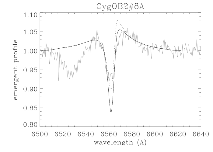
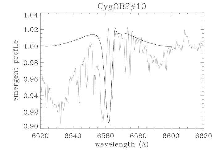
Figure 15: As Fig. 13, but for objects with “intermediate” H_α-profile type.

In the following, we will give, where necessary, some comments on the fits for the invidual objects. All results have been summarized in Table 7. The fits for objects with H_α in emission are displayed in Figs. 13 and 14, for objects with “intermediate” H_α profile types in Fig. 15, and for objects with H_α in absorption in Figs. 16 and 17.

B.1 Objects with H_α in emission

Cyg OB2#7.

For the hottest object in our sample, only upper limits for the radio fluxes are available. The derived mass-loss rate is consequently an upper limit as well (and the clumping factors corresponding lower limits), and based on the assumption that this star is a thermal emitter. By means of our regression (Eq. 4), helium is predicted to remain doubly ionized throughout the entire wind (this is the only object in our sample for which this is so), whereas specific models within our grid (located in the relevant parameter range) indicate that helium might still recombine in the outermost, radio-emitting region. Thus we have derived two solutions for this object, both for an ionized and a recombined radio regime.

For the doubly ionized solution, we derive a (maximum) mass-loss rate of 2.8$\cdot 10^{-6}\,{\rm M_{\odot}/yr}$. The lower wind is strongly clumped to a similar degree in regions 2 and 3 ($f_{\rm cl}^{\rm in}=10$ and $f_{\rm cl}^{\rm mid}=8{\ldots}12$, respectively. The lower value for $f_{\rm cl}^{\rm mid}$ results in a good fit of the 10 $\mu{\rm m}$ flux, but slightly too narrow wings of H_α, whereas with $f_{\rm cl}^{\rm mid}=12$ we can fit these wings perfectly, but somewhat overestimate the 10 $\mu{\rm m}$ flux. As for the unclumped models (Mokiem et al. 2005), the absorption trough cannot be fitted well by models with $\beta\leq 0.9$ (nebular emission?), though the wings are nicely matched. If we assume, on the other hand, that the trough is refilled by the wind alone, the complete profile can be reproduced with $\beta\approx 1$ and $f_{\rm cl}^{\rm in}=8,f_{\rm cl}^{\rm mid}=10{\ldots}12$, respectively. From the shape of the trough we derive $r_{\rm in}\la 1.1$, otherwise it becomes too narrow or too deep.

The alternative solution with helium recombined in the radio region yields a considerable larger mass-loss rate, ${\dot{M}}$= 4$\cdot 10^{-6}\,{\rm M_{\odot}/yr}$, since we have adopted a large helium content, $Y_{\rm He}$=0.21 (compare with the case of $\zeta$ Pup; see Sect. 4.1). All clumping properties scale accordingly, and the best solution (for $\beta$=0.9) is obtained with $f_{\rm cl}^{\rm in}=5$ and $f_{\rm cl}^{\rm mid}=4{\ldots}6$. Since the 10 $\mu{\rm m}$ flux indicates that helium is not completely ionized, even in the outermost IR photosphere (otherwise it would lie somewhat higher), we prefer the recombined model for our final solution (see Table 7). In the corresponding fit diagram, we have indicated both possibilities though (solid: recombined; dotted: ionized).

HD 190429A.

For this object, there are two measurements at 3.5 cm which are considerably different, namely 200 $\mu$J (our observations) and 280 $\mu$J from Scuderi et al. (1998). As is obvious from the fit diagram, the 6 cm flux (our measurement) is consistent with the unpublished 3.5 cm value provided by Scuderi et al., whereas it lies too high with respect to our 3.5 cm measurements. Thus, either the star is strongly variable, or a non-thermal emitter, or the errors estimated for our observations are too optimistic. Note that the 0.7 cm measurement (upper limit) is consistent with our 3.5 cm flux. A “wrong” assumption concerning the He recombination cannot explain this dilemma: if the ionization degree was higher than predicted, the 0.7 cm flux would be most affected and would lie at a level higher than actually observed.

On the assumption that we see thermal emission and that the discrepancy is due to measurement problems, the maximum mass-loss rate is constrained to lie between 7.5 (dotted) and 9.5$\cdot 10^{-6}\,{\rm M_{\odot}/yr}$ (solid), and both limits have been indicated in Table 7. By adjustment of the clumping factors, we obtain a perfect fit for H_α. If the 0.7 cm flux is not much lower than its upper limit, $f_{\rm cl}^{\rm out}$ must be lower than, or equal to, 2. The only other discrepancy found for this object concerns the 4.63 $\mu$m measurement from Castor & Simon (1983), which cannot be matched by any of our models.

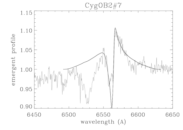
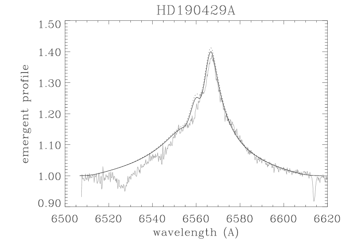
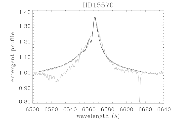
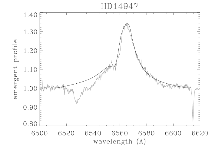
Figure 13: Fit diagrams (left: H_α profile; right: IR/radio continua) for objects with H_α in emission. Arrows indicate upper limits. For parameters, see Table 7. Alternative solutions (dotted, dashed) are discussed in the comments on individual objects in Appendix B.

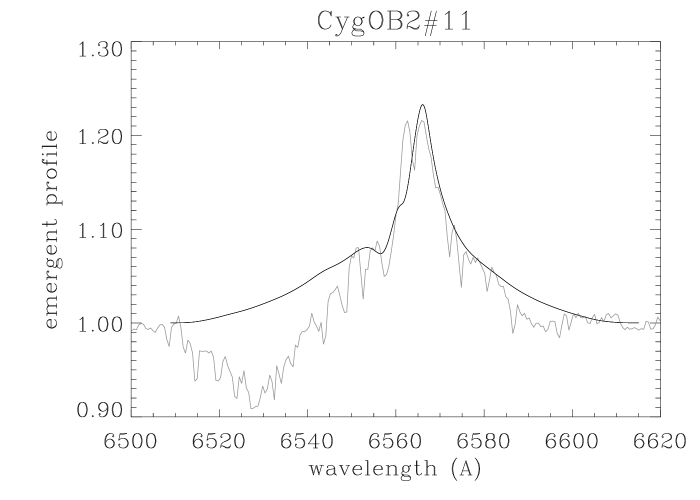
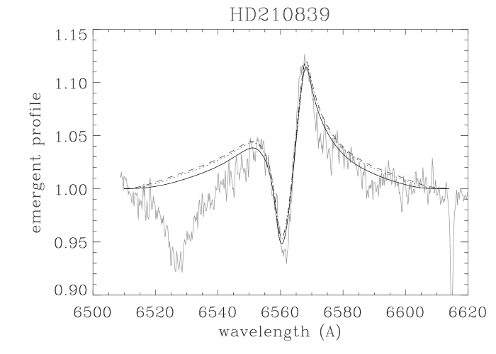
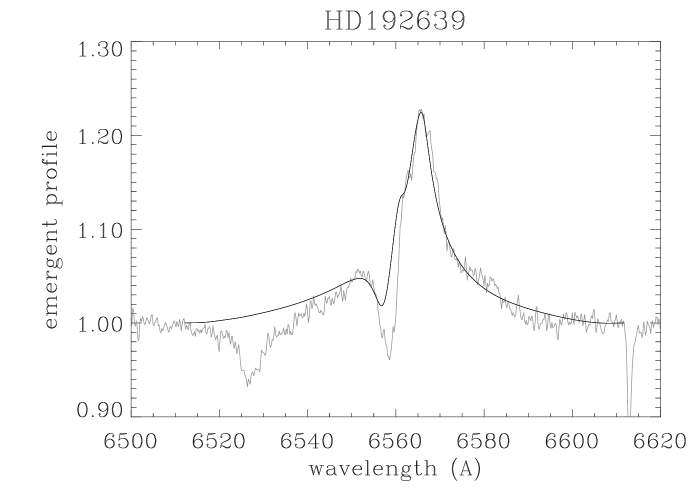
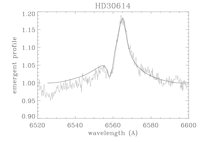
Figure 14: As Fig. 13.

HD 15570

can be fitted without any problems, and the only complication arises because of the large error bars attributed to the scuba fluxes. Since, for the corresponding wavelength, it is not completely clear whether He is already recombined or not, we have investigated both possibilities. In the recombined case (which is consistent with our predictions: recombination at 6.3 $R_{\ast}$, 1.3mm radiation becoming optically thick at 9.5 $R_{\ast}$), the wind must be significantly clumped in region 4 ($f_{\rm cl}^{\rm out}=5{\ldots}20$); larger values can be excluded from the H_α wings. If, on the other hand, the wind is not recombined in the 1.3 mm-forming region, a value of $f_{\rm cl}^{\rm out}=1$ is still consistent with the limit of the scuba data. The clumping in region 3 ($f_{\rm cl}^{\rm mid}=6$) is well-constrained from the H_α line wings, though a lower value, $f_{\rm cl}^{\rm mid}=4$, results when we force the 10 $\mu$m flux to be matched. In the latter case then, H_α becomes a bit too narrow.

Note that the two measurements at 3.5 cm almost overlap (but not completely, indicating a certain variability), and we have forced our solution to comply with their average value. In the fit diagram, we have plotted three solutions which are consistent with the error bars for the scuba measurements: $f_{\rm cl}^{\rm out}=5$ (dotted), $f_{\rm cl}^{\rm out}=13$ (solid) and $f_{\rm cl}^{\rm out}=20$ (dashed). To find even closer constraints on the outer wind clumping requires lower error bars. Additional far-IR observations (though being important as consistency checks) will not help to improve this uncertainty, since the far-IR is insensitive to any reasonable variation of $f_{\rm cl}^{\rm out}$ for this object.

HD 66811

has been already discussed in some detail; see Sect. 4.1.

HD 14947.

The 3.5 cm flux is well determined (with some variability), whereas only upper limits are available at 2 and 6 cm. The resulting mass-loss rate is ${\dot{M}}$ = 8…12 $\cdot 10^{-6}\,{\rm M_{\odot}/yr}$, and H_α can be perfectly fitted, with rather low clumping factors in the lower wind. In the fit diagram and Table 7, we have indicated the intermediate solution with ${\dot{M}}$ = 10$\cdot 10^{-6}\,{\rm M_{\odot}/yr}$ and clumping factors $f_{\rm cl}^{\rm in}$ = 3.1 and $f_{\rm cl}^{\rm mid}$ = 2.5.

Cyg OB2#11

has similar clumping properties to HD 14947, and the maximum mass-loss rate can be derived to within small errors: ${\dot{M}}$ = 5 $\pm$ 0.5 $\cdot 10^{-6}\,{\rm M_{\odot}/yr}$. From H_α, the potentially unclumped region must be located within $r_{\rm in}\la 1.2$. From the line wings, $f_{\rm cl}^{\rm mid}$ is somewhat larger than $f_{\rm cl}^{\rm in}$, and $f_{\rm cl}^{\rm out}$ might be tightly constrained if far-IR observations were available. Problems for this object concern the blue side of the H_α emission being predicted as too narrow, and the 10.9 $\mu$m flux (Leitherer et al. 1982), which cannot be matched by any of our models.

HD 210839.

Though the error bars for the scuba fluxes are smaller than for HD 15570, two different, barely overlapping fluxes have been measured, which might introduce a twofold solution for region 4, though the maximum mass-loss rate is well defined.

A first solution (solid) can be derived for the lower scuba measurement, with constant clumping in the lower wind, $f_{\rm cl}^{\rm in}$ = $f_{\rm cl}^{\rm mid}$ = 6.5 until $r_{\rm out}$ = 10, and no clumping in the outer part. The upper scuba measurement can be fitted by additional clumping in region 4, with $f_{\rm cl}^{\rm out}$ = 5…20, but in this case the 0.7 cm flux appears as too large.

A second, slightly better solution (which is indicated in Table 7) can be found if one assumes constant clumping (again with $f_{\rm cl}=6.5$) until $r<4$, and a larger clumping factor of $f_{\rm cl}=10$ until $r<15$. With $f_{\rm cl}^{\rm out}$ = 1, the lower 1.3 mm flux is matched (dotted), whereas with $f_{\rm cl}^{\rm out}$ = 8 the upper one can be fitted (dashed). As before, however, the 0.7 cm flux is then predicted as too large. For all solutions, H_α is perfectly reproduced, and a value of $r_{\rm in}\la 1.2$ can be constrained from its trough.

HD 192639.

Only one radio measurement is available, and only as an upper limit. Adopting this value and assuming thermal emission, the maximum mass-loss rate can be restricted to ${\dot{M}}$ $\la$ 3$\cdot 10^{-6}\,{\rm M_{\odot}/yr}$, with constant clumping factors, $f_{\rm cl}^{\rm in}=f_{\rm cl}^{\rm mid}=3.5$, in the lower wind, and $r_{\rm in}\la 1.1$. For all our simulations, the observed 4.63 $\mu$m flux (taken from Castor & Simon 1983) is smaller than synthesized, though better reproduced than for HD 190420A, and independent of the ionization equilibrium for helium.

HD 30614

is perfectly matched, both in the radio and in H_α, with a moderate degree of clumping in the inner and intermediate wind.

B.2 Objects with “intermediate” H_α profile type

Cyg OB2#8A

is a confirmed non-thermal radio emitter (Bieging et al. 1989). In order to obtain at least an estimate, as low a maximum mass-loss rate as possible has been adopted (from the 2 cm flux), although this might still be even smaller, of course. With $\beta$ = 0.74 (taken from the optical analysis using homogeneous models, Mokiem et al. 2005), the wings of H_α are fitted best, whereas the absorption becomes too deep. A value of $\beta$ = 0.85 (dotted) improves the trough, but the emission then becomes too large. The 20 $\mu$m flux indicates that our prediction for the recombination radius of helium might be erroneous, and a completely recombined model (which at these temperatures is rather improbable) can indeed fit this measurement. Only low clumping factors are required to fit H_α, though higher values would be necessary if the mass-loss rate were lower. Note that with $f_{\rm cl}^{\rm mid}=2.0$ the wings of H_α are nicely matched, but the 10 $\mu$m flux is slightly overestimated. With $f_{\rm cl}^{\rm mid}=1$, on the other hand, the latter problem can be cured, at the expense of H_α.

Cyg OB2#10

can be fitted accounting for weak clumping in the lower wind ($f_{\rm cl}^{\rm in}=1.4$, $f_{\rm cl}^{\rm mid}=1.8$) if $\beta$ is left at its nominal value of 1.05. $r_{\rm in}$ must be $\la 1.2$, and clumping effects are seen only in the inner wind. The observed 10 $\mu$m flux is larger than predicted, which cannot be corrected for by a non-recombined wind, as the temperature is too low for such a scenario.

B.3 Objects with H_α in absorption

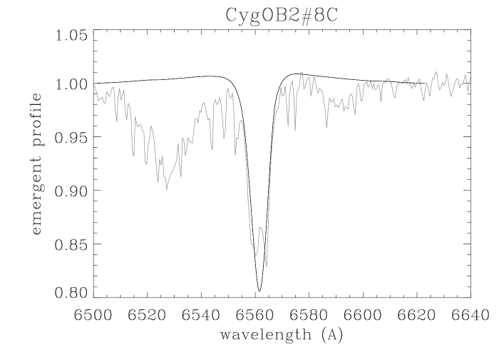
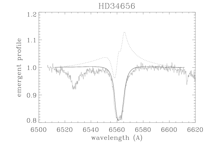
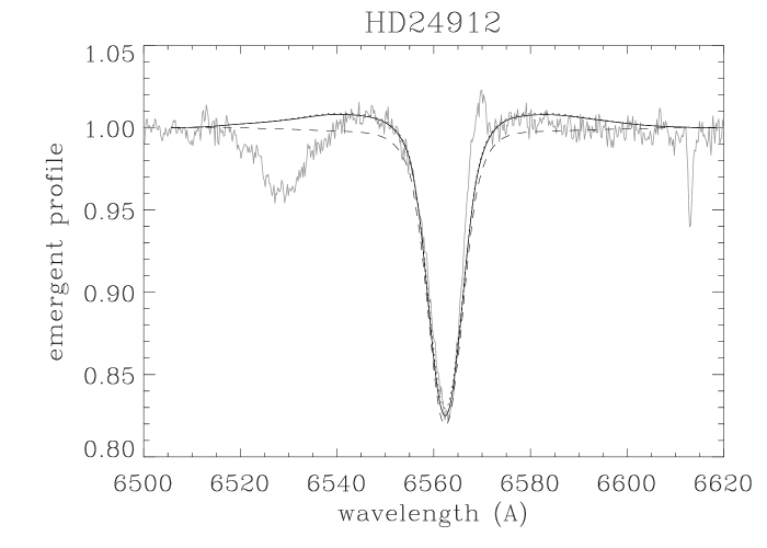
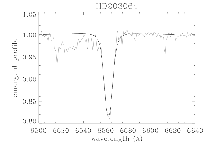
Figure 16: As Fig. 13, but for objects with H_α in absorption.

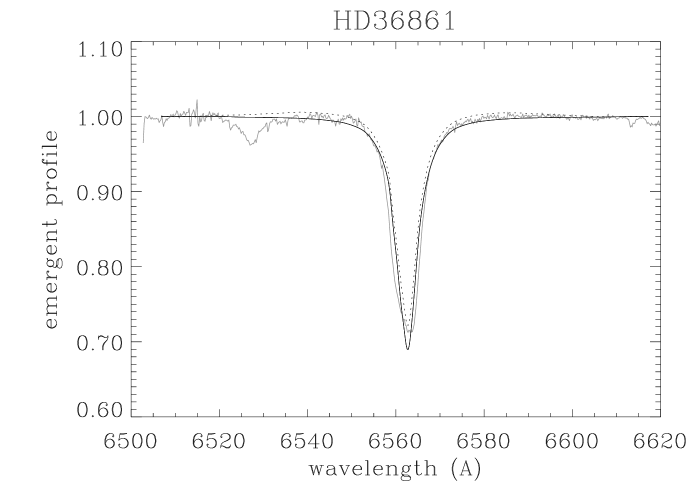
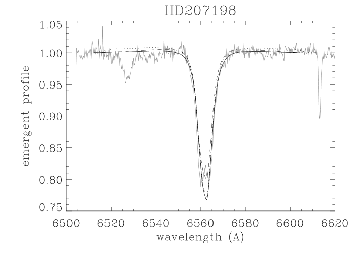
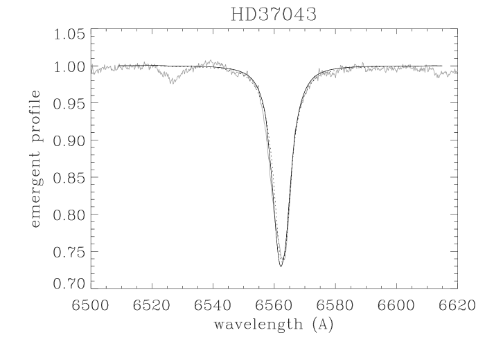
Figure 17: As Fig. 16.

For all objects with H_α in absorption, we have used $r_{\rm out}=10$, since due to the lower wind density, the IR and radio emission is formed at smaller distances from the star (cf. Sect. 4.1). E.g., for HD 36861, the wind becomes optically thick at 2 cm only for $r\la 10R_{\star}$.

Cyg OB2#8C

remains rather unconstrained by our analysis, since only one upper limit in the radio range is available (at 6 cm), and this upper limit yields a mass-loss rate larger than the one derived from H_α (${\dot{M}}$= 3.5$\cdot 10^{-6}\,{\rm M_{\odot}/yr}$ for $\beta=1$). Thus, the largest possible mass-loss rate has been adopted from this value, and the only definite statement concerns $f_{\rm cl}^{\rm mid}$ being similar to $f_{\rm cl}^{\rm in}$.

HD 34656

is the only object within our sample where the radio mass-loss rate (if thermal emission) is definitely larger than the H_α mass-loss rate. Unfortunately, only one measurement (at 3.5 cm) provides a hard number, whereas the 2 and 6 cm measurements yield upper limits only. Thus, non-thermal emission cannot be excluded, at least to some extent, if one compares the 3.5 and 6 cm fluxes (Fig. 16). Besides being a non-thermal emitter, there are two other possibilities: either the 3.5 cm measurements are somewhat corrupted (i.e., can be regarded as upper limits only), or the outer wind is more heavily clumped than the inner one. In the latter case, the maximum mass-loss rate results from H_α instead of from the radio, and corresponds to 3$\cdot 10^{-6}\,{\rm M_{\odot}/yr}$ for $\beta=1$, which is the lowest possible value such that $\beta$ remains consistent with our data (wings of H_α). Note that a value of $\beta=1.1$ and ${\dot{M}}$ = 2.6$\cdot 10^{-6}\,{\rm M_{\odot}/yr}$, as derived in Paper I, gives a slightly better solution. Since the (thermal) radio mass-loss rate corresponds to a value of 7$\cdot 10^{-6}\,{\rm M_{\odot}/yr}$ (and would result in an emission profile for H_α; cf. the dotted solution), clumping factors of $f_{\rm cl}^{\rm far}=(\dot{M}_{\rm radio}/\dot{M}_{\rm H\alpha})^{2}\approx 6$ are necessary to obtain a simultaneous fit, with $f_{\rm cl}^{\rm mid}$ = $f_{\rm cl}^{\rm in}$ being well-constrained.

HD 24912.

All radio fluxes measured for $\xi$ Per are upper limits. Our fit diagram shows that the 0.7, 2 and 6 cm limits, if taken at face value, are consistent with thermal emission and a maximum mass-loss rate of 2.3$\cdot 10^{-6}\,{\rm M_{\odot}/yr}$, which is very close to the value provided by Repolust et al. (2004), using unclumped models. When accounting additionally for the 3.5 cm flux, one derives a maximum mass-loss rate of 1.2$\cdot 10^{-6}\,{\rm M_{\odot}/yr}$. In the following we will consider both possibilities.

The solution with larger ${\dot{M}}$ requires weak clumping in the lowermost wind ($f_{\rm cl}^{\rm in}=2.1$), and additional clumping in region 3 ($f_{\rm cl}^{\rm mid}$ = 5), if the small emission humps on the red and blue side of the H_α absorption are due to clumping and not to other processes (see below). The maximum value of $f_{\rm cl}^{\rm out}$ is restricted by $f_{\rm cl}^{\rm out}\la 2$, otherwise the radio band becomes affected and the maximum mass-loss rate must be decreased.

The lower ${\dot{M}}$ solution (which is consistent with all radio measurements) requires considerable clumping in the lower wind. Assuming a “standard value” of $\beta=0.9$ (which has been used for most of the following objects as well, but see Sect. 4.3), $f_{\rm cl}^{\rm in}=8$ and $f_{\rm cl}^{\rm mid}\la 20..25$, the humps can be explained by clumping. Furthermore, the unclumped region (if any) can be constrained by $r_{\rm in}\la 1.1$. For this solution, $f_{\rm cl}^{\rm out}\la 3$, otherwise ${\dot{M}}$ is even lower. In our fit diagrams, we have plotted the high ${\dot{M}}$ solution (solid), the low ${\dot{M}}$ solution (dotted) and the low ${\dot{M}}$ solution with $f_{\rm cl}^{\rm mid}=1$, which does not fit the emission humps in H_α. At least this uncertainty might be resolved if future far-IR measurements become available.

Let us comment finally on the strong excess measured in the mid-IR, between 8.7 to 11.4 $\mu$m (taken from Gehrz et al. 1974), which is in stark contrast to the 12 $\mu$m IRAS data from Beichman et al. (1988). This discrepancy (see also Sect. 6) cannot be due to a wrong flux calibration, since measurements from the same source have been used also for HD 30614 and HD 36861, without any apparent problems. Thus, $\xi$ Per is either strongly variable in the mid-IR, or the mid-IR excess is due to another physical process (e.g., co-rotating interaction zones, see de Jong et al. 2001, or a wind compressed equatorial region). The latter interpretation in particular is consistent with the red and blue emission humps observed in H_α, which have also been seen in Heii 4686 (Herrero et al. 1992, Fig. 4).

HD 203064.

For the standard value of $\beta=0.9$, a model with all clumping factors being unity is consistent with the observations. Values for $f_{\rm cl}^{\rm mid}\ga 2$ can be excluded.

HD 36861.

All radio measurements provide only upper limits, and we have indicated a model with a consistent maximum mass-loss rate, ${\dot{M}}$ = 0.4$\cdot 10^{-6}\,{\rm M_{\odot}/yr}$. For this value and $\beta$ = 0.9, the innermost clumping is weak again, $f_{\rm cl}^{\rm in}$ = 2…4, and $f_{\rm cl}^{\rm mid}$ must be lower than 20 (from the wings of H_α). Solutions with $f_{\rm cl}^{\rm out}>2$ are no longer consistent with the adopted mass-loss rate. In Fig. 17, we have indicated the solutions with minimum ($f_{\rm cl}^{\rm in}=2,f_{\rm cl}^{\rm mid}=1$, solid) and maximum ($f_{\rm cl}^{\rm in}=4,f_{\rm cl}^{\rm mid}=20$, dotted) clumping. Note that only far-IR or mm observations will help to disentangle this uncertainty.

HD 207198

has well-defined radio measurements, and an unclumped wind with ${\dot{M}}$ = 1.0…1.2$\cdot 10^{-6}\,{\rm M_{\odot}/yr}$ (for $\beta=0.9$) matches all observational constraints ($f_{\rm cl}^{\rm mid}\la 2$). The 2 cm flux can be reproduced with $f_{\rm cl}^{\rm out}=10$ (and $<$15); larger values are excluded by the H_α wings. Displayed are the solutions for an unclumped wind at ${\dot{M}}$ = 1.0$\cdot 10^{-6}\,{\rm M_{\odot}/yr}$ (solid), a wind with additional clumping in the outer region ($f_{\rm cl}^{\rm out}=10$, dotted) and a homogeneous wind with ${\dot{M}}$ = 1.2$\cdot 10^{-6}\,{\rm M_{\odot}/yr}$ (dashed).

HD 37043.

By inspection of the measured radio fluxes, this star is either a non-thermal emitter (SB2!), or the 6 cm flux is erroneous. At 3.5 cm, we have two measurements which are consistent. To obtain more conclusive results, one needs to re-observe this star in the radio range.

Nevertheless, we present two solutions: an upper one discarding the 3.5 cm data and being consistent with the upper limit at 2 cm, and a lower, more likely one (which would also be an upper limit if the object were a non-thermal emitter), discarding the 6 cm measurement.

In the first case, ${\dot{M}}$ = 0.8$\cdot 10^{-6}\,{\rm M_{\odot}/yr}$, and a smooth wind is consistent with the observations. In the second case, ${\dot{M}}$ = 0.25$\cdot 10^{-6}\,{\rm M_{\odot}/yr}$, and the wind is strongly clumped at least in the lowermost wind, with $f_{\rm cl}^{\rm in}=12$ for $r_{\rm in}=1{\ldots}1.05$ to $r_{\rm mid}\la 1.3$. Due to the low density, clumping in other regions has a very low impact on the model fluxes, and we can exclude only values $f_{\rm cl}^{\rm mid}>20$ and $f_{\rm cl}^{\rm out}>10$ (otherwise the maximum mass-loss rate must be lower). Plotted are the “smooth” solution with the upper value for ${\dot{M}}$ (solid), and the lower ${\dot{M}}$ solution, which is strongly clumped (dotted).

HD 209975

has already been discussed in Sect. 4.1.