A Time-Symmetric Block Time-Step Algorithm for N-Body Simulations

Abstract

The method of choice for integrating the equations of motion of the general N-body problem has been to use an individual time step scheme. For the sake of efficiency, block time steps have been the most popular, where all time step sizes are smaller than a maximum time step size by an integer power of two. We present the first successful attempt to construct a time-symmetric integration scheme, based on block time steps. We demonstrate how our scheme shows a vastly better long-time behavior of energy errors, in the form of a random walk rather than a linear drift. Increasing the number of particles makes the improvement even more pronounced.

1 Introduction

For long-term N-body simulations, it is essential that the drift in the values of conserved quantities is kept to a minimum. The total energy is often used as an indicator of such a drift. During the last fifteen years, two approaches have been put forward to improve numerical conservation of energy and other theoretically conserved quantities: symplectic integration schemes, where the simulated system is guaranteed to follow a slightly perturbed Hamiltonian system, and time-symmetric integration schemes, where the simulated system follows the same trajectory in phase space, when run backward or forward

In both cases, for symplectic as well as for time-symmetric schemes, the introduction of adaptive time steps tends to destroy the desired properties. Symplectic schemes are perturbed to different Hamiltonians at different choices of time step length, and therefore lose their global symplecticity. Time-symmetric schemes typically determine their time step length at the beginning of a step, which implies that running a step backward gives a slightly different length for that step. See Leimkuhler & Reich (2005) for a recent review of various attempts to remedy this situation.

In practice, many large-scale simulations in stellar dynamics use a block time-step approach, where the only allowed values for the time step length are powers of two (Aarseth, 2003). The name derives from the fact that, with this recipe, many particles will share the same step size, which implies that their orbit integration can be performed in parallel. An added benefit, in the case of individual time steps, is the fact that block time steps allow one to predict the positions of all particles only once per block time step, rather than separately for each particle that needs to be moved forward. Since parallelization is rapidly becoming essential for any major simulation, we explore in this paper the possibility to extend time symmetry to the use of block time steps.

In Section 2, we analyze some of the problems that occur when applying existing methods to the case of block time steps, and we offer a novel solution, with a truly time symmetric choice of time step, with the restriction that we only allow changes of a factor two in the direction of increasing and decreasing the time step. In Section 3, we present numerical tests of our new scheme in the simplest case of the 2-body problem, which already shows the superiority of our approach over various alternatives. In Section 4, we demonstrate that the advantage carries over to the general N-body problem. Section 5 sums up.

2 Block Time Steps

2.1 Implicit Iterative Time Symmetrization

It is surprisingly easy to introduce a time-symmetric version for any adaptive self-starting integration scheme. Let $\xi=(r,v)$ be the $2N$-dimensional phase space vector for a system with $N$ degrees of freedom, and let $f(\xi_{i},\delta t_{i})$ be the operator that maps the phase space vector of the system at time $t_{i}$ to a new phase space vector at time $t_{i+1}=t_{i}+\delta t_{i}$. Any choice of self-starting integration scheme, together with a recipe to determine the next time step $\delta t_{i}$, at time $t_{i}$ and phase space value $\xi_{i}(t_{i})$, defines the precise form of $f(\xi_{i},\delta t_{i})$.

The recipe for making any such scheme time-symmetric was given by Hut, Makino & McMillan (1995), as:

$$\left\{\begin{array}[]{lcl}\xi_{i+1}&=&f(\xi_{i},\delta t_{i}),\\ \phantom{1}&\phantom{1}&\phantom{1}\\ \delta t_{i}&=&{\displaystyle\frac{h(\xi_{i})+h(\xi_{i+1})}{2}}\end{array}\right.$$ (1)

where $h(\xi)$ can be any time step criterion. Note that this recipe leads to an implicit integration scheme, which can be solved most easily through iteration. In practice, one or two iterations suffice to get excellent accuracy, but at the cost of doubling or tripling the number of force calculations that need to be performed. Extensions of this implicit symmetrization idea have been presented by Funato et al. (1996) and Hut et al. (1997).

Since we will need to inspect the idea of iteration below in more detail, let us write out the process here explicitly. We start with the given state $\xi_{i}$ and the implicit equation for $\xi_{i+1}$ of the form

$$\xi_{i+1}=f(\xi_{i},\delta t_{i}(\xi_{i},\xi_{i+1}))$$ (2)

The first guess for $\xi_{i+1}$ is

$$\xi_{i+1}^{(0)}=f(\xi_{i},\delta t_{i}(\xi_{i},\xi_{i}))$$ (3)

and we can consider this as our zeroth-order iteration. With this guess in hand, we can now start to iterate, finding

$$\xi_{i+1}^{(1)}=f(\xi_{i},\delta t_{i}(\xi_{i},\xi_{i+1}^{(0)}))$$ (4)

as our first-order iteration. This will already be much closer to the final value, as long as the time steps are small enough and the function $\delta t_{i}$ does not fluctuate too rapidly. In general, the $k^{th}$ iteration will yield a value for $\xi_{i+1}$ of

$$\xi_{i+1}^{(k)}=f(\xi_{i},\delta t_{i}(\xi_{i},\xi_{i+1}^{(k-1)}))$$ (5)

We will now consider the application of these techniques to block time steps. For the purpose of illustrating the use of block time steps, it will suffice to use the leapfrog scheme (also known as the Verlet-Störmer-Delambre scheme, according to the authors who rediscovered this scheme at roughly century-long intervals), which we present here in a self-starting, but still time-symmetric form:

$$r_{i+1} = r_{i}+v_{i}\delta t+a_{i}(\delta t)^{2}/2$$

$$v_{i+1} = v_{i}+(a_{i}+a_{i+1})\delta t/2$$ (6)

All our considerations carry over to higher-order schemes, as long as the base scheme can be made time-symmetric when iterated to convergence. An example of such a scheme is the widely used Hermite scheme(Makino, 1991).

2.2 Flip-Flop Problem

To start with, we apply the recipe of Hut, Makino & McMillan (1995) to block time steps. Let us define a block time step at level $n$ as having a length:

$$\Delta t_{n}=\frac{\Delta t_{1}}{2^{n-1}}.$$ (7)

where $\Delta t_{1}$ is the maximum time step length. Starting with the continuum choice of

$$\delta t_{c,i}=\frac{h(\xi_{i})+h(\xi_{i+1})}{2}$$ (8)

we now force each time step to take on the block value $\delta t_{i}=\Delta t_{n}$ for the smallest $n$ value that obeys the condition $\Delta t_{n}\leq\delta t_{c,i}$. In more formal terms, $\delta t_{i}=\delta t_{i}(\delta t_{c,i})=\Delta t_{n}$ for the unique $n$ value for which

$$n=\min_{k\geq 1}\left\{k\ \Big{|}\ \frac{1}{2^{k-1}}\leq\frac{h(\xi_{i})+h(\xi_{i+1})}{2}\right\}$$ (9)

The problem with this approach is that we are no longer guaranteed to find convergence for our iteration process, as can be seen from the following example. Let $h(\xi_{i})=0.502$ and let the time derivative of $h(\xi_{i}(t))$ along the orbit be $(d/dt)h(\xi_{i}(t))=-0.01$. We then get the following results for our attempt at iteration.

$$\xi_{i+1}^{(0)} = f(\xi_{i},\delta t_{i}(\xi_{i},\xi_{i}))=f(\xi_{i},\delta t_{i}(h(\xi_{i})))$$ (10)

$$= f(\xi_{i},\delta t_{i}(0.502))=f(\xi_{i},0.5)$$

$$\xi_{i+1}^{(1)} = f(\xi_{i},\delta t_{i}(\xi_{i},\xi_{i+1}^{0}))=f(\xi_{i},\delta t_{i}([h(\xi_{i})+h(\xi_{i+1}^{0})]/2))$$ (11)

$$= f(\xi_{i},\delta t_{i}([0.502+(0.502+0.5*(-0.01))]/2))$$

$$= f(\xi_{i},\delta t_{i}([0.502+0.497]/2))$$

$$= f(\xi_{i},\delta t_{i}(0.4995))=f(\xi_{i},0.25)$$

$$\xi_{i+1}^{(2)} = f(\xi_{i},\delta t_{i}(\xi_{i},\xi_{i+1}^{1}))=f(\xi_{i},\delta t_{i}([h(\xi_{i})+h(\xi_{i+1}^{1})]/2))$$ (12)

$$= f(\xi_{i},\delta t_{i}([0.502+(0.502+0.25*(-0.01))]/2))$$

$$= f(\xi_{i},\delta t_{i}([0.502+0.4995]/2))$$

$$= f(\xi_{i},\delta t_{i}(0.50075))=f(\xi_{i},0.5)$$

And from here on, $\xi_{i+1}^{(k)}=f(\xi_{i},0.25)$ for every odd value of $k$ and $\xi_{i+1}^{(k)}=f(\xi_{i},0.5)$ for every even value of $k$: the process of iteration will never converge.

Under realistic conditions, for slowly varying $h$ functions and small time steps, this flip-flop behavior will not occur often, but it will occur sometimes, for a non-negligible fraction of the time. We can see this already from the above example: for a linear decrease in the $h$ function of $(d/dt)h(\xi_{i}(t))=-0.01$, we will get flip-flopping not only for $h(\xi_{i})=0.502$ but for any value in the finite range $0.50125<h(\xi_{i})<0.5025$.

Since iteration converges correctly over the rest of the interval $0.5<h(\xi_{i})<1$, we conclude that in this particular case flip-flopping occurs about one quarter of one percent of the time, over this interval. This is far too frequent to be negligible in a realistic situation.

Clearly, a straightforward extension of the implicit iterative time symmetrization approach does not work for block time steps, because iteration does not converge. We have to add some feature, in some way. Our first attempt at a solution is to take the smallest of the two values in a flip-flop situation.

2.3 Flip-Flop Resolution

The most straightforward solution of the flip-flop dilemma is like cutting the Gordian knot: we just take the lowest value of the two alternate states. The drawback of this solution is that in general we need at least two iterations for each time step, to make sure that we have spotted, and then correctly treated, all flip-flop situation. In general, it is only at the third iteration that it becomes obvious that a flip-flop is occurring. To see this, consider the previous example with a starting value of $h(\xi_{i})=0.501$. In that case we will get $\xi_{i+1}^{(0)}=f(\xi_{i},0.5)$ and $\xi_{i+1}^{(1)}=f(\xi_{i},0.25)$, just as when we started with $h(\xi_{i})=0.502$. The difference shows up only at the second iteration, where we now find $\xi_{i+1}^{(2)}=f(\xi_{i},0.25)$, a value that will hold for all higher iterations as well.

The original iterative approach to time symmetry in practice already gives good results when we use only one iteration. This implies a penalty, in terms of force calculations per time steps, of a factor two compared to non-time-symmetric explicit integration. Now the use of flip-flop resolution will force us to always take at least two iterations per step, raising the penalty to become at least a factor of three.

However, there is a more serious problem: there is still no guarantee that taking the lowest value in a flip-flop situation leads to a time-symmetric recipe. In fact, what is even more important, we have not yet checked whether our symmetric block time-step scheme is really time symmetric, in the absence of flip-flop complications.

In order to investigate these questions, let us return to the example we used above, but instead of a linear time derivative, let us now use a quadratic time derivative for the $h$ function that gives the estimate for the time step size. Rather than writing a formal definition, let us just state the values, while shifting the time scale so that $t=0$ coincides with the particle position being $\xi_{i}$:

$$h(0.00) = 0.502$$

$$h(0.25) = 0.499$$

$$h(0.50) = 0.499$$ (13)

When we start at time $t=0$, and we integrate forward, we find:

$$\xi_{i+1}^{(0)} = f(\xi_{i},\delta t_{i}(\xi_{i},\xi_{i}))=f(\xi_{i},\delta t_{i}(h(\xi_{i})))$$ (14)

$$= f(\xi_{i},\delta t_{i}(0.502))=f(\xi_{i},0.5)$$

$$\xi_{i+1}^{(1)} = f(\xi_{i},\delta t_{i}(\xi_{i},\xi_{i+1}^{0}))=f(\xi_{i},\delta t_{i}([h(\xi_{i})+h(\xi_{i+1}^{0})]/2))$$ (15)

$$= f(\xi_{i},\delta t_{i}([0.502+0.499]/2))$$

$$= f(\xi_{i},\delta t_{i}(0.5005))=f(\xi_{i},0.5)$$

and so on: all further $k$th iterations will result in $\xi_{i+k}^{(1)}=f(\xi_{i},0.5)$. There is no flip-flop situation, when moving forward in time.

However, when we now turn the clock backward, after taking this step of half a time unit, we start with the value $h(0.50)=0.499$, which leads to a first step back of $\delta t=0.25$. The end point of the first step back is $t=0.25$ with $h(0.25)=0.499$. Therefore, also here there is no flip-flop situation: all iterations, while going backward, result in a time step size of $\delta t=0.25$.

We have thus constructed a counter example, where forward integration would proceed with time step $\delta t=0.5$ and subsequent backward integration would proceed with time step $\delta t=0.25$. Clearly, our scheme is not yet time symmetric, even in the absence of a flip-flop case.

2.4 A First Attempt at a Solution

Let us rethink the whole procedure. The basic problem has been that the very first step in any of our algorithms proposed so far has not been time symmetric. The very first step moves forward, and leads to a newly evolved system at the end of the first step. Only after making such a trial integration, do we look back, and try to restore symmetry. However, as we have seen, the danger is large that this trial integration is not exhaustive: it may already go too far, or not far enough, and thereby it may simply overlook a type of move that the same algorithm would make if we would start out in the time-reversed direction.

Formulating the problem in this way, immediately suggests a solution. At any point in time, let us first try to make the largest step that is allowed. If that step turns out to be too large for our algorithm, we try a step that is half that size. if that step is too large still, we again half the size, and so on, until we find a step size that agrees with our algorithm, when evaluated in both time directions. A similar treatment has been described by Quin et al (1997).

This type of approach is clearly more symmetric than what we have attempted so far. Instead of using information of the physical system at the starting point of the next integration step, we only use a mathematical criterion to find the largest time step size allowed at that point, and we then apply the physical criteria symmetrically in both directions.

Let us give an example. If the largest time step size is chosen to be unity, then at time $t=0$ we start by considering this time step. We try, in this order $\delta t=1$, $\delta t=0.5$, $\delta t=0.25$, and so on, until we find a time step for which integration starting in the forward direction, and integration starting in the backward direction, both result in the new time step being acceptable. Let us say that this is the case for $\delta t=0.125$.

After taking this step, we are at time $t=0.125$. The largest time step allowed at that point, forward or backward, is $\delta t=0.125$. Any larger time step would result in non-alignment of the block time steps: in the backward direction it would jump over $t=0$. So at this point we start by considering once more $\delta t=0.125$. If that time step is too large, we try half that time step, halving it successively until we find a satisfactory time step size.

Imagine that the second time step size is also $\delta t=0.125$. In that case, we land at $t=0.25$. From there on, the maximum allowed time step size is $\delta t=0.25$, so the first try should be that size.

In principle, this approach seems to be really time symmetric. However, there is a huge problem with this type of scheme, as we have just formulated it. Imagine the system to crawl along with time steps of, say $\delta t=1/1024$, and reaching time $t=1$. Our new recipe then suggests to start by trying $\delta t=1$, a 1024-fold increase in time step! Whatever subtle physical effect it was that forced us to take such small time steps, is completely ignored by the mathematical recipe that forces us to look at such a ridiculously large time step.

For example, in the case of stellar dynamics, a double star may force the stars that orbit each other to take time steps that are necessarily far shorter than the orbital period. Starting out with a trial step size that is far larger than an orbital period may or may not give spuriously safe-looking results. Clearly, we have to exclude such enormous jumps in time step.

2.5 A Second Attempt at a Solution

The simplest solution to taming sudden unphysical increases in time steps is to allow at most an increase of a factor two, in either the forward or the backward direction. This then implies that we can only allow decreases of a factor two, and not more than two, in either direction. The reason is that a decrease of a factor four in one direction in time would automatically translate into an increase of a factor four in the other direction.

Note that we have to be careful with our time step criterion. If we allow time steps that are too large, we may encounter situations where our time step criterion would suggest us to shrink time steps by a factor of four, from one step to the other. Since our algorithm does not allow this, we can at most shrink by a factor of two, which may imply an unacceptably large step. However, if our time step criterion is sufficiently strict, allowing only reasonably small time steps too start with, it will be able to resolve the gradients in the criterion in such as way as to handle all changes gracefully through halving and doubling.

When we apply this restriction to the scheme outlined in the previous subsection, we arrive at the following compact algorithm.

First a matter of notation. Any block time step, of size $\delta t=1/2^{k}$, connects two points in time, only one of which can be written at $t=Z/2^{(k-1)}$, with $Z$ an integer. Let us call that time value an even time, from the point of view of the given time step size, and let us call that other time value an odd time. To give an example, if $\delta t=0.125$, than $t=0,0.25,0.5,0.75,1$ are all even times, while $t=0.125,0.375,0.625,0.875$ are all odd times.

Here is our algorithm:

• When we start in a given direction direction in time, at a given point in time, we should determine the time step size of the last step made by the system. In that way, we can determine whether the current time is even or odd, with respect to that last time step.

• If the current time is odd, our one and only choice is: to continue with the same size time step, or to halve the time step. First, we try to continue with the same time step. If, upon iteration, that time step qualifies according to the time-symmetry criterion used before, Eq. 9, we continue to use the same time step size as was used in the previous time step. If not, we use half of the previous time step.

• If the current time step is even, we have a choice between three options for the new time step size: doubling the previous time step size, keeping it the same, or halving it. We first try the largest value, given by doubling. If Eq.9 shows us that this larger time step is not too large, we accept it, otherwise we consider keeping the time step size the same. If Eq.9 shows us that keeping the time step size the same is okay, we accept that choice, otherwise we just halve the time step, in which case no further testing is needed.

Note that in this scheme, we always start with the largest possible candidate value for the time step size. Subsequently, we may consider smaller values, but the direction of consideration is always from larger to smaller, never from smaller to larger. This guarantees that we do not run into the flip-flop problem mentioned above.

3 Numerical Tests for the 2-Body Problem

Figure 1: Relative energy errors for a two-body integration of a bound orbit with eccentricity $e=0.99$. The top line with highest slope corresponds to algorithm 1, the line with intermediate slope corresponds to algorithm 2, and below those the two lines for algorithms 0 and 3 are indistinguishable in this figure.

Figure 2: Relative energy errors at apocenter. The four lines, from top to bottom, correspond to algorithms 1, 2, 3, and 0.

Figure 3: Same as Fig. 2, but for a duration that is ten times longer.

We present here the results for a gravitational two-body integration. The relative orbit of the two point masses forms an ellipse with an eccentricity of $e=0.99$. We have chosen a time unit such that the period of the orbit is $T=2\pi$.

We have implemented four different integration schemes:

0) the original time-symmetric integration scheme described by Hut, Makino & McMillan (1995), where there is a continuous choice of time step size. This is the approach described in section 2.1. We have used five iterations for each step.

1) a block-time-step generalization, with a fixed number of iterations. This is the approach analyzed in section 2.2. Here, too, we chose five iterations for each step.

2) a block time step generalization, with a variable number of iterations. If after five iterations, the fourth and the fifth iterations still give a different block time step size, then we choose the smallest of the two. This recipe avoids flip-flop situations. It is the approach described in section 2.3.

The algorithm described in the next section, 2.4, we have not implemented here, because it is guaranteed to lead to large errors in those cases where a new large time step is allowed again just before pericenter passage. We therefore switched directly to the following section:

3) the implementation of our favorite algorithm, where we start with a truly time symmetric choice of time step, with the restrictions that we only allow changes of a factor two in the direction of increasing and decreasing the time step, and that we only allow an increase of time step on the so-called even time boundaries. This is the approach given in section 2.5.

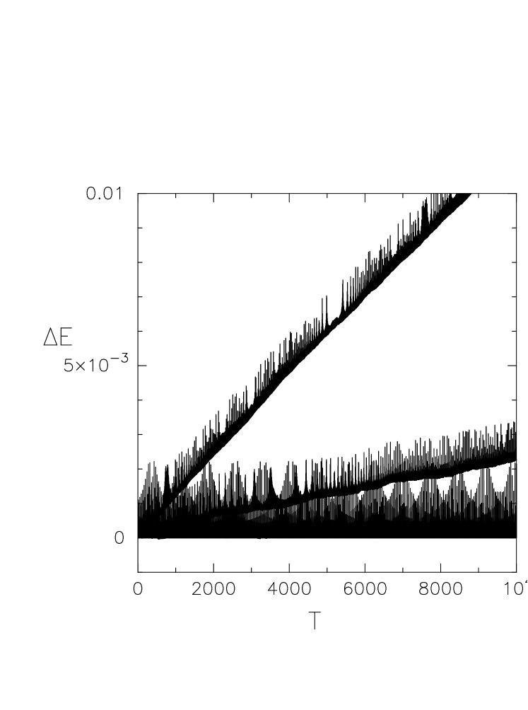
In figures 1 and 2 we show the results of integrating our highly eccentric binary with these four integration schemes. In each case, the largest errors are produced by algorithm 1), smaller errors are produced by algorithm 2), and even smaller errors appear with algorithm 3). Finally, algorithm 0) gives the smallest errors.

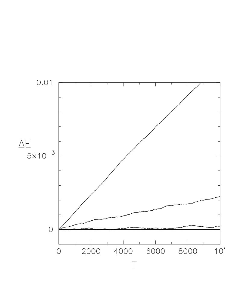
Figure 1 shows the energy error in the two-body integration as a function of time. As is generally the case for time-symmetric integration, the errors that occur during one orbit are far larger than the systematic error that is generated during a full orbit. To bring this out more clearly, figure 2 shows the error only one time per orbit, at apocenter, the point in the orbit where the two particles are separated furthest from each other, and the error is the smallest.

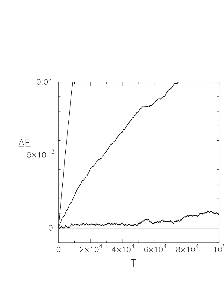
Finally, figure 3 shows the same data as figure 2, but for a period of time that is ten times longer. In both figures 2 and 3, it is clear that the first two block time steps algorithms, 1) and 2), both show a linear drift in energy. This is a clear sign of the fact that they violate time symmetry. Note that in both figures algorithm 3) gives rise to a time dependency that looks like a random walk. This may well be the best that can be done with block time steps, when we require time symmetry.

4 N-body implementation

So far, we have discussed the implementation of our block-symmetric algorithm for individual time steps in the case of the two-body problem. Of course, for $N=2$, it is not really necessary to use block time steps, nor is it useful to introduce individual time steps. The reason we made both of these extensions was to implement and test our basic ideas in the simplest case. In this section, we describe and test our algorithm for the general $N$-body problem.

4.1 Divide and Conquer: the Concept of an Era

The major conceptual difficulty in designing a time-symmetric block step scheme is the global context information that is needed, with extensions toward the future as well as the past. In order to determine the time step for particle $i$ at time $t$, we need the information of all other particles $j$ at that time. In general, there will be at least some $j$ values for which the position and velocity of particle $j$ are not given at time $t$, because particle $j$ has a time step larger than particle $i$ and time $t$ happens to fall within the duration of one time step for particle $j$.

In such a case, the time step of particle $i$ at time $t$ depends on the positions and velocities of other particles $j$, that can only be determined from time symmetric interpolation between the positions and velocities of each particle $j$ at times earlier and later than $t$. However, the future $j$ positions and velocities depend in turn on the orbit of particle $i$, and thus on the time step of particle $i$ at time $t$. In other words, there is a circular dependence between the future positions and velocities of particles $j$ and the time step of particle $i$.

To make things worse, each of the future positions and velocities of any of the particles in turn will depend on information that is given even further in the future. If we continue this logic, we would have to know the complete future of a whole simulation, before we could attempt to time symmetrize that whole history. And while any simulation will stop at a finite time, so the number of time steps for each particle will be a finite number, it is clearly unpractical to let the very first time step depends on the positions and velocities of the particles at the very end of simulation.

A more practical solution is to impose a maximum size for any time step, as $\Delta t_{max}$. If we start the simulation at time $t_{0}$, we know that all particles will reach time $t_{1}=t_{0}+\Delta t_{max}$, by making one or more steps. At that time, all particles will be synchronized. This means that we can focus on time symmetric orbit integration for all particles during the interval $[t_{0},t_{1}]$, without the need for any information about any particle at any time $t>t_{1}$.

In other words, we divide and conquer: we split the total history of our simulation into a number of smaller periods, which we call eras. Each era extends a period in time equal to the largest allowed time step $\Delta t_{max}$, or to an integer multiple of $\Delta t_{max}$, whatever turns out to be the most convenient.

4.2 Era-Based Iteration

Let the beginning of a single era be $t_{0}$ and the end $t_{1}$. As we saw above, in order to obtain the time step size for particle $i$ at time $t$ within our era, we typically need to know the positions and velocities of some other particles at times larger than $t$. The simplest way to provide this future information is through iteration.

First we just perform standard forward integration, with the usual kind of non-time-symmetric block step algorithm, for the complete duration of our era ($t_{0}<t<t_{1}$). While simultaneously integrating the orbits of all particles, we store the positions and velocities (and if necessary higher order time derivatives) for all time steps for all particles during our era. This will then allow us to obtain the position and velocity of any particle at any arbitrary time through interpolation, to the accuracy given by this first try, which will function as our zeroth iteration.

Next we make our first iteration. We again perform orbit integration for our complete $N$-body system, during $t_{0}<t<t_{1}$. However, there are two differences with respect to the first try. First of all, in order to calculate the force from particle $j$ on particle $i$, we no longer extrapolate the orbit of particle $j$ to the time requested by $i$, but instead we interpolate the position and velocity of particle $j$ to the requested time, using stored positions and velocities of particle $j$ at slightly earlier and later times, using a time symmetric interpolation scheme. Secondly, we can now begin to symmetrize the time step for particle $i$, in the same way as we did it for the two-body problem in the previous section, with one exception: we now obtain the estimated time step size at the beginning of the time step from the current iteration, and we obtain the estimated time step size at the end of the time step from the previous iteration (in the two-body case the iteration was done separately for each step).

Subsequent attempts, as second and higher iterations, repeat the same steps as the first iteration.

As before, we have implemented our iteratively time symmetric block step algorithm using the leapfrog algorithm as our basic integrator. Generalizations to higher-order schemes are somewhat more complex, but follow the same basic logic we are outlining in the current paper. We have adopted the following time step criterion for particle $i$:

$$\delta t_{i}=\eta\ {\rm min}_{j}\frac{|r_{ij}|}{|v_{ij}|},$$ (16)

where $\eta$ is a constant parameter and $r_{ij}$ and $v_{ij}$ are the relative position and velocity between particles $i$ and $j$. To symmetrize the time step, we simply require that the step sizes that would be determined by the above criterion at both ends of the time step are not smaller than the actual time step used. In other words, we take the minimum of the two time step values that our criterion gives us at the beginning and at the end of the time step; this minimum is our symmetrized time step. We could have taken the average, but here we have used the minimum value, for simplicity.

4.3 Numerical Results for $N=100$ and $N=512$

Figure 4: Growth of the relative energy error for 100-body runs, starting from twenty different sets of initial conditions. For each set of initial conditions, two integrations have been performed, one without and one with time-symmetrization (in the latter case, using six iterations). The twenty lines with time symmetrization form the horizontal bundle which is slowly spreading in square-root-of-time fashion like a random walk; the twenty lines without time symmetrization all show a systematic, near-linear decrease in energy.

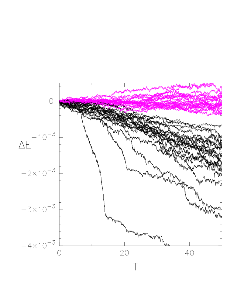
Figure 4 show how the energy errors grow in the 100-body problem. In each case, we started with random realizations of a Plummer model, where we used standard $N$-body units, in which the gravitational constant $G=1$, the total mass $M=1$ and the total energy is $E_{tot}=-1/4$. We have integrated each system for 50 time units, with a maximum time step of $1/64$ and $\eta=0.1$ (see Eq. 16). We have used standard Plummer type softening with softening length $\epsilon=0.01$. We have carried out forty time integrations, starting from twenty different realizations of the Plummer model. For each realization, we have integrated the system once without any time symmetrization and once with time symmetrization using six iterations to guarantee sufficient convergence. In our experience, at least three iterations were necessary to achieve high accuracy.

It is clear that all runs without time symmetry show a systematic drift in energy, while no such systematic tendency is visible for time symmetrized runs. Among the twenty non-symmetrized runs, even the best result came out worse than the worst result among the symmetrized runs. We conclude that time symmetrization can significantly improve the long-term accuracy of $N$-body simulations.

Figure 5: Growth of the relative energy error for 512-body runs, starting from a single set of initial conditions, but using a different number of iterations. The lowest curve presents an integration without time symmetrization. The curve above that presents the result of time symmetrization using only one iteration. The next two curves show the results of using three and two iterations, respectively; initially, the third iteration curve rises a bit above the second iteration curve.

Figure 6: Growth of the relative energy error for 512-body runs, like figure 5, but starting from a different set of initial conditions. As before, the lowest curve presents an integration without time symmetrization, and the curve above that presents the result of time symmetrization using only one iteration. The second iteration curve is the one that stays above the third iteration curve for most of the run depicted here.

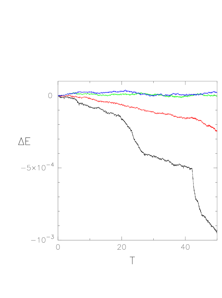
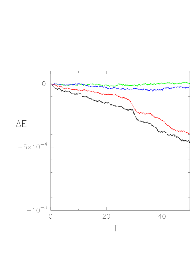
Figure 5 shows similar results for 512-body runs. Here we have started from a single Plummer model realization, and the curves show the effect of varying the number of iterations. In this case, the second and third iteration already show a dramatic improvement in the long-time behavior of the total energy of the system. The softening used here is $\epsilon=1/512$. All other parameters are the same as for the 100-body runs. For the 512-body case, the improvement is significantly better than it was in the 100-body runs. Finally, figure 6 shows that the results depicted in figure 5 are generic: starting from a different set of initial conditions changes the details but not the overall picture, and again the second and third iterations show dramatic improvements over the original run and the first iteration.

We offer the following explanation for the increase in accuracy of the time-symmetric scheme as a function of particle number. In these runs, contributions to the error are largely generated by close encounters between two particles, since the softening we used is relatively small. These error contributions are dominated by weak encounters, since the softening, while small, is not small enough to make gravitational focusing significant. The number of weak encounters that take place during one time unit, within a particle-particle distance that is less than the inter-particle distance (of order $N^{1/3}$) is of order $O(N^{4/3})$. If our time symmetrization succeeds in replacing the systematic effects of all these encounters by a random effect, the result will be a shift from a linear to a square root drift, effectively replacing the $O(N^{4/3})$ dependence by a $O(N^{2/3})$ dependence. We conclude that the relative reduction in the total energy error, due to time symmetrization, grows with $N$, as $N^{2/3}$.

Whether or not time-symmetric integration is to be preferred, depends on the number of particles and the duration of the integration. In the example case shown in figure 4, the energy error is about a factor of 10 smaller for time-symmetric integration, but the same effect could be achieved in a computationally cheaper way by reducing the step size by a factor of $\sqrt{10}$. For large $N$, however, as shown already in figure 5, the effect of time symmetry is more pronounced.

For very long integrations, time-symmetric integration is clearly better, since in that case the error grows in random-walk fashion, as $\sqrt{t}$, while for any non-time-symmetric scheme scheme the error grows linearly, proportional to $t$. In the case of a star-cluster simulation which covers many relaxation timescales, the particles in the core can go through a very large number of crossing times. For example, a simulation of a globular cluster with $10^{6}$ stars would need to cover at least $10^{5}$ half-mass crossing times. The crossing timescale in the core is at least a factor of 100 shorter than that of the half-mass crossing time. Therefore, particles in the core need to be followed for as many as $10^{7}$ local crossing times. The difference between the scaling of $\sqrt{t}$ and $t$ produces a improvement of a factor of roughly $10^{3.5}$ in the energy error, in the case of time-symmetric integration. With a second-order scheme, this translates into a factor of 100 difference in the necessary step size. Even with a fourth-order scheme, it would imply a difference of a factor of ten in the time step. Clearly, even applying five iterations will produce a gain of a factor two with respect to the alternative of having to decrease the time step by a factor of ten.

4.4 Description of the Algorithm

Here we describe the algorithm in some more detail. To enable the reader to check the precise implementation of our algorithm, we have made available the computer code used to generate figures 4, 5, and 6, on our Art of Computational Science web site

Consider the integration of the system from time $t_{0}$ to $t_{1}$. We can assume for simplicity that the zero point in time has been chosen in such a way as to be compatible with the era size, so that both $t_{0}$ and $t_{1}$ are integer multiples of the time interval $t_{1}-t_{0}$.

In the first pass through this era, we integrate all particles with the standard block step scheme, without any intention to make the scheme time symmetric. In the calculations reported in this paper, we have used the same predictor-corrector form of the leapfrog algorithm as mentioned earlier in Eq. 6:

$$r_{new} = r_{old}+v_{old}\Delta t+\frac{1}{2}a_{old}\Delta t^{2},$$

$$v_{new} = v_{old}+\frac{1}{2}(a_{old}+a_{new})\Delta t.$$ (17)

As we discussed before, if one particle $i$ wants to step forward in time, we need to know the positions of all particles $j$ in order to compute the force that each particle $j$ exerts on particle $i$. Among the particles $j$, many may have a larger time step than particle $i$, so we may have to predict the position for such a particle, for the time at which particle $i$ wants to make a step. In addition, we need to predict the velocity of particle $j$, because the velocity difference between particles $i$ and $j$ are used in determining the time step size, according to Eq. 16.

The predicted position $r_{p,\;j}$ for particle $j$ is obtained with a second-order Taylor expansion, while for the predicted velocity $v_{p,\;j}$ a first-order expansion suffices:

$$r_{p,\;j} = r_{j}+v_{j}(t-t_{j})+\frac{1}{2}a_{j}(t-t_{j})^{2},$$

$$v_{p,\;j} = v_{j}+a_{j}(t-t_{j}),$$ (18)

The integrated positions and velocities for each particle $i$ at each time step, $r_{new}$ and $v_{new}$ in Eq. 17, are all stored.

In the next iteration, we proceed in the same way, but the time step is calculated differently. At time $t$ for particle $i$, let the time step calculated according to the criterion (16) be $\delta t$, and the time step not exceeding this $\delta t$ and compatible with the block step criterion be $\Delta t_{p}$. But now we would like to know the time step size that would be required at the end of this step, at time $t^{\prime}=t+\Delta t_{p}$.

There are two possibilities. If particle $i$ ended a time step at time $t^{\prime}$ in the previous iteration, we are in luck, and we can use the same procedure we used in the two-body case. To be specific, we test if the time step according to criterion (16) is smaller than $\Delta t_{p}$; if so, we halve the value of $\Delta t_{p}$. However, if we are not in luck, and we do not have time $t^{\prime}$ in the list of times for which particle $i$ was integrated in the previous iteration, we simply adopt the time step that we obtained looking in the forward direction. In that case, we have to wait till a next iteration, to apply the time symmetrization procedure. This occasional miss explains why the iteration procedure often requires several iterations before accurate time symmetry can be obtained.

To calculate the force at the new time for particle $i$, we use the positions of the other particles $j$ calculated by interpolation, based on the previous iteration, in the following way. The interpolation itself is done in a straightforward, linear way. However, since we have a more accurate position at hand for at least the starting point of each orbit segment, for particle $j$, we may as well correct the old orbit segment by shifting it rigidly by an amount equal to the difference between the starting point of the current and the previous iteration.

To be specific, the interpolated position at time $t$ for particle $j$ is given by

$$r_{p}=(1-f)r_{s}+fr_{e}+\Delta r_{s},$$ (19)

where $f=(t-t_{s})/(t_{e}-t_{s})$, $t_{s}$ is the largest time in the list of times for particle $j$ not exceeding $t$ and $t_{e}$ is the next time in that list, immediately following $t_{s}$. Here both $r_{s}$ and $r_{e}$ are obtained from the stored results from the previous iteration. The correction term $\Delta r_{s}$ is defined as

$$\Delta r_{s}=r_{s,new}-r_{s},$$ (20)

where $r_{s,new}$ is the position of particle $j$ at time $t_{s}$ in the current iteration. As in the case described above, sometimes we are unlucky, and $r_{s,new}$ is not available. In that case we just set $\Delta r_{s}$ to be zero, postponing further accuracy improvement until the next iteration.

To make our predictor-corrector form of the leapfrog integration scheme consistent, we use the same interpolation scheme for the predictor part, for the particles to be integrated. For the corrector part, we used the trapezoidal scheme, as follows:

$$v_{c,new} = v_{old}+\frac{1}{2}\Delta t(a_{old}+a_{new}),$$ (21)

$$r_{c,new} = r_{old}+\frac{1}{2}\Delta t(v_{old}+v_{c,new}).$$ (22)

Here, the subscript old refers to the value at the previous time, the subscript c,new refers to the corrected value at the new time, $a_{old}$ is calculated with the old values for the positions, and $a_{new}$ is calculated with the predicted values of the positions. Note that the first corrected quantity that can be computed is $v_{c,new}$, based on the old and predicted quantities. After that, we can also compute the corrected quantity $r_{c,new}$, based on the old quantities and $v_{c,new}$.

5 Discussion

We have succeeded in constructing an algorithm for time symmetrizing block time steps that does not show a linear growth of energy errors. As far as we know, this is the first such algorithm that has been discovered. We expect this algorithm to have practical value for a wide range of large-scale parallel N-body simulations. While we have illustrated our approach for simplicity with the leapfrog scheme, all our considerations carry over to higher-order schemes, as long as the base scheme can be made time-symmetric when iterated to convergence. An example of such a scheme is the widely used Hermite scheme(Makino, 1991). We plan to discuss such applications in a future paper.

A major novelty in our scheme has been the introduction of a time period, which we can an era, during which all positions and velocities of all particles are stored in memory. These values are retained from one iteration to the next. We expect that this procedure will have other advantages as well, in that it prevents sudden surprises to occur. For example, if a particle will suddenly require a very high speed, it may approach another particle with a long time step without any warning. As another example, a star may undergo a supernova explosion, something that other particles will normally only notice when there current time step has finished. In both cases, after the first iteration all particles will have access to full knowledge about these unexpected events, and during the iteration procedure, they can automatically adapt to the new situation.

Our new scheme promises to be competitive with traditional non-symmetrized schemes, especially for very long integration times, in that the same error bounds may be reached using less computer time. To prove that this will be the case for realistic applications clearly requires further detailed investigations, beyond the scope of the current paper. The memory use of our scheme may seem formidable, and indeed, when a large value for the era size is chosen, memory use is increased significantly over traditional schemes. For those N-body calculations that are CPU time limited, this may not be much of a concern. However, for large-scale cosmological simulations and other applications for which memory is important, it is possible to choose an era size in such a way that the memory requirement of the new scheme is less than twice the memory requirement of non-symmetric schemes, at a CPU performance penalty of less than a factor two. Here the trick is to take an era size close to the harmonic mean of the time steps of all particles. In that way, half the computing cost of the non-symmetric scheme is associated with particles that have time steps shorter than this era size. Those particles with natural time steps longer than this era choice will see their step size shortened to the era size, but the total increase in time steps will be less than a factor two.

The reason that our scheme shows a dramatic improvement in accuracy is time symmetry, which suppresses linear error growth. The reason that our scheme is somewhat complicated is purely empirical: all else failed, in our attempts to try simpler schemes. Whether our procedure is the simplest scheme that actually can produce time symmetric versions of block time step codes is an open question. It may well be, but we certainly have no mathematical proof. This is an interesting question to be pursued further, for theoretical as well as practical reasons.

We acknowledge conversations with Joachim Stadel at the IPAM workshop on N-Body Problems in Astrophysics, in April 2005, where he presented a time symmetric version of the preprint by Quinn et al. (1997) which is similar to our first attempt at a solution, described in section 2.4. We thank Sverre Aarseth, Mehmet Atakan Gürkan, and an anonymous referee for their comments on the manuscript. M.K. and H.S. acknowledge research support from ITU-Sun CEAET grant 5009-2003-03. P.H. thanks Prof. Ninomiya for his kind hospitality at the Yukawa Institute at Kyoto University, through the Grants-in-Aid for Scientific Research on Priority Areas, number 763, ”Dynamics of Strings and Fields”, from the Ministry of Education, Culture, Sports, Science and Technology, Japan.

References

- (1)
- Aarseth (2003) Aarseth, J., S., 2003, Gravitational N-Body Simulations, Cambridge University Press.
- Hut et al. (1997) Hut, P., Funato, Y., Kokubo, E., Makino, J. & McMillan, S., 1997, Time Symmetrization Meta-Algorithms, in Computational Astrophysics, eds. D. A. Clarke and M. J. West, ASP Conference Series, Vol. 123 (San Francisco: ASP), pp. 26-31.
- Funato et al. (1996) Funato, Y., Hut, P., McMillan, S. & Makino, J., 1996, Time-Symmetrized Kustaanheimo-Stiefel Regularization, Astron. J. 112, 1697-1708.
- Hut, Makino & McMillan (1995) Hut, P., Makino, J. & McMillan, S., 1995, Building A Better Leapfrog, Astrophysical Journal 443, L93-L96.
- Leimkuhler & Reich (2005) Leimkuhler, B. & Reich, S., 2005, Simulating Hamiltonian Dynamics, Cambridge University Press.
- Makino (1991) Makino, J., 1991, Optimal Order and Time-Step Criterion for Aarseth-Type N-body Integrations, Astrophysical Journal 369, 200-212.
- Quinn et al. (1997) Quinn, T., Katz, N., Stadel, J. & Lake, G., 1997, Time stepping N-body simulations, preprint, archived on http://arxiv.org/ps/astro-ph/9710043.