McScatter: a Simple Three-Body Scattering Package with Stellar Evolution

Abstract

We describe a simple computer package which illustrates a method of combining stellar dynamics with stellar evolution. Though the method is intended for elaborate applications (especially the dynamical evolution of rich star clusters) it is illustrated here in the context of three-body scattering, i.e. interactions between a binary star and a field of single stars. We describe the interface between the dynamics and the two independent packages which describe the internal evolution of single stars and binaries. We also give an example application, and introduce a stand alone utility for the visual presentation of simulation results.

1 Introduction

Many methods exist for modelling the dynamical evolution of rich star clusters (see Heggie & Hut 2003, ch.9), but very few include anything other than the crudest model of stellar evolution. Indeed realistic evolution of single and binary stars is confined to the $N$-body codes developed by Aarseth and colleagues (Aarseth 2004) and those included in the starlab package (Portegies Zwart et al 2001, Appendix B). For the efficient modelling of globular star clusters, faster methods are desirable, but none yet incorporates stellar and binary evolution of any sophistication (see however Portegies Zwart et al. 1997; Ivanova et al.  2004). Our aim in this paper is to facilitate this development, by showing how the stellar evolution modules in $N$-body codes can be incorporated into other codes. For this purpose we have developed a very simple package, called McScatter, which simulates the evolution of a single binary in dynamical interactions with a field of single stars. Exchanges are allowed, and therefore all essential aspects of dynamics which affect binaries in star cluster simulations are incorporated. We begin with a description of the dynamics, and then proceed to those aspects of the stellar and binary evolution modules which have to be understood for our purposes. The code we are describing is publicly available at http://manybody.org/manybody/McScatter.html .

2 Description of McScatter

The main purpose of McScatter is to illustrate how stellar evolution is to be interfaced with stellar dynamics. We describe the dynamical part in outline only (in the following subsection). Subsequent subsections describe the interface with the stellar evolution packages in somewhat greater detail.

The essential structure of the code is a loop (Table 1) in which it is decided whether or not a significant scattering event occurs within a timestep. The timestep size is selected based on the encounter rate and the evolutionary state of the binary. If no scattering event occurs during the selected timestep the binary is evolved to the current time and the new timestep is determined. On the other hand, if a scattering event occurs with a single star of some mass selected from the initial mass function, this star is then evolved to the time of the encounter, as explained in § 2.1.

Note that, if a binary is affected (e.g. by exchange) in any encounter, the updating of the binary takes place during the following pass through the main loop. This is done only in order to keep the updating of the binary parameters in one place in the code.

Table 1: Flow-Chart

Initialize binary with primary mass, secondary mass,
                       semi-major axis and eccentricity.
compute maximum encounter rate

loop for a Hubble time
BEGIN
  determine time step (dt)
  check whether encounter occurs in this timestep with third body of
ΨZAMS mass (m): set flag SCATTER and encounter time
  update binary parameters for previous encounter (if flagged)
  evolve binary to time (t+dt) or time of encounter

  if(SCATTER == TRUE)
  BEGIN
    evolve encountering star to moment of encounter
          (note that the mass that was set was the ZAMS mass; it
           may be affected by stellar evolution.)
    perform scatter between binary and third star
    print intermediate result
  END
  print final result
END

2.1 Dynamics

We adopt a very simple scattering cross section $\Sigma$, based on the geometrical cross section of the binary and gravitational focusing, and normalised to give the correct result in the well studied case of equal masses, i.e.

$$\Sigma=\frac{5\pi}{16}\sqrt{\frac{\pi}{3}}\frac{AGM_{123}a}{V^{2}},$$ (1)

where $A=21$ (Spitzer 1987, Sec.6.1b), $G$ is the constant of gravitation, $M_{123}$ is the sum of the masses of the stars participating in the 3-body encounter, $a$ is the semi-major axis of the binary, and $V$ is the relative speed (at infinity) of the third star and the centre of mass of the binary.

For the single stars we assume a power law initial mass function

$$f(m)dm\propto m^{-\alpha}dm$$

between some minimum $m_{-}$ and upper limit $m_{+}$, and a space number density $n$. We suppose that $V$ has a Maxwellian distribution in equipartition, in the sense that, if $\sigma$ is the one-dimensional velocity dispersion of stars of average mass ${\langle m\rangle}$, the mean square value of $V$ is

$$\langle V^{2}\rangle=\frac{3\mbox{${\langle m\rangle}$}M_{123}}{M_{12}m_{3}}\sigma^{2},$$

where $M_{12},m_{3}$ are the total mass of the binary and the mass of the single star, respectively.

From these formulae the code estimates an upper bound on the rate of encounters, and we choose the time step $\delta t$ so that the corresponding average number of encounters is less than $0.1$. The following simple rejection method then determines simultaneously, for the current time step, whether an encounter occurs, and the value of $m_{3}$. The procedure uses the fact that the probability of occurrence of an encounter is

$$P=\delta t\int_{m_{-}}^{m_{+}}\langle\Sigma V\rangle nf(m_{3})dm_{3},$$ (2)

where the average is taken over the distribution of $V$. Two random numbers $X,Y$ are chosen independently from uniform distributions on the ranges $(m_{-},m_{+})$ and $(0,1)$, respectively, and an encounter with $m_{3}=X$ is deemed to occur if $Y$ is smaller than the integrand in eq.(2)

If an encounter occurs, the time of the encounter is chosen randomly within the time step, and the evolution of the binary and the encountering star are updated. (An error is committed here, because the evolution will change the assumed mass of the encountering star and possibly the orbital parameters of the binary.) The manner in which the stellar evolution is implemented is discussed in subsequent sections. Here we mention the remaining steps of the dynamical evolution.

The adopted probability of an exchange is based on results of Heggie, Hut & McMillan (1996). For simplicity we ignore the exponential correction term in their eq.(17). This then gives an approximation for the cross section for exchanging the first component, normalised by an expression proportional to the right side of our eq.(1). Therefore it can be interpreted as being proportional to the probability of exchange, given that an encounter has occurred. We normalise this expression so that the probability of exchange of one specific component is $1/3$ for equal masses. The sum of the resulting probabilities of exchanging either component may exceed unity (if $m_{3}$ is very large) and in such a case we reduce both probabilities so that their sum is unity.

If an exchange has occurred the total mass of the binary tends to increase. In this case we keep $a$ unchanged, and the increase in mass hardens the binary. If there is no exchange the binding energy of the binary is increased in accordance with the differential cross section given by Spitzer (1987, eq.[6-27]). The new eccentricity is chosen randomly from the thermal distribution.

2.2 Stellar Evolution

Before any encounter takes place the evolution of the binary has to be initialised and the first single star given a unique identifier. Whenever an encounter is scheduled to take place, the evolution of both the binary and the single star are updated to the time of the encounter. If, during this evolution step, the binary is dissociated by a supernova or if the two stars coalesce, we stop the simulation. Otherwise, after the evolution step the orbital parameters of the binary ($a$ and $e$) and the masses ($m_{1}$ and $m_{2}$) of the two stars are returned to the dynamical part of the code.

Then the stellar evolution of the new third body is initialised. It is evolved to the moment the encounter is scheduled and the stellar parameters are computed. Then we continue by implementing the encounter, as described in the previous section.

We consider two distinct stellar/binary evolution modules. The first is SeBa  (Portegies Zwart et al. 2001) which is part of the starlab package and provides stellar and binary evolution for the kira $N$-body code. The second is BSE (Hurley, Tout & Pols 2002) which provides the same function for the NBODY4 code (Aarseth 2004). Both of these modules also work as stand-alone binary population synthesis packages. In each case the binary evolution is prescription based – in order to facilitate the rapid computation of many binaries – although there are differences in the implementation (see references and Section 3.1). For SeBa  the underlying stellar evolution is provided by the evolution formulae presented by Eggleton, Fitchett & Tout (1989) while BSE uses the SSE stellar evolution package (Hurley, Pols & Tout 2000).

2.3 The Interface

The interface between the dynamics and the stellar evolution is separated from both program parts. Though written in C++ (SeBa) or Fortran (BSE) it can be linked-in to either FORTRAN, C, C++, etc.  code. The interface is limited to specific operations which are generally required for the communication. These include routines to pass or request information, force an update and request for update times. See the Appendix for details.

3 Application

3.1 The evolution of a single binary in a dense star cluster

McScatter is meant merely to illustrate how to construct an interface between a dynamical code and SeBa  or BSE. It is not intended for dynamical investigations, for which a much more carefully constructed code would be needed (cf. Ivanova et al 2004). Nevertheless the following exercise illustrates in a qualitative way some of the interactions between dynamics and stellar evolution

We use the code which has been presented in this paper to model a particular binary in the core of a large star cluster, in a similar environment as is presented in Portegies Zwart et al. (1997), where binary-binary encounters are ignored. For initial binary parameters we select the semi-major axis $a=4000$ ${\rm R}_{\odot}$  eccentricity $e=0.6$, primary and secondary masses $M=2$ ${\rm M}_{\odot}$, and $m=1$ ${\rm M}_{\odot}$, respectively. In isolation this binary evolves in about 9.8 Gyr (11.2 Gyr) to a pair of carbon-oxygen white dwarfs with masses 0.64 ${\rm M}_{\odot}$  (0.64 ${\rm M}_{\odot}$) and 0.54 ${\rm M}_{\odot}$  (0.52 ${\rm M}_{\odot}$) with semi-major axis $a\simeq 10,200$ ${\rm R}_{\odot}$(8600 ${\rm R}_{\odot}$). Interestingly enough the simulation with BSE (in brackets) resulted in a slightly reduced eccentricity of 0.55, whereas SeBa  reported no change. This change is mainly caused by differences in the treatment of tidal circularization, and also largely explains the difference in the final semi-major axes. (See fig. 4 for a graphic presentation of the binary evolution for SeBa). The evolution timescales also differ and this is directly related to the distinct nature of the evolution prescriptions. For example, the SSE package used in BSE was constructed from stellar models that included convective overshooting and updated opacity tables in comparison to the Eggleton, Fitchett & Tout (1989) models used by SeBa. We note that solar metalicity is assumed for the stars in our chosen binary.

Now we evolve this binary with McScatter with a stellar density of the background population ranging from $n=100$pc^-3 to $n\simeq 10^{5}$pc^-3, and velocity dispersion $\sigma=10$ km s^-1. For each selected density we initialize the binary $10^{3}$ times and evolve it against a background of single stars, which are taken from a Salpeter initial mass function between 0.1 ${\rm M}_{\odot}$  and 100 ${\rm M}_{\odot}$. In figure 1 we show the mean of the final orbital separation of the binary after a 12 Gyr evolution in a cluster as a function of the background density. Each simulation takes less than 2 seconds with either code for the above mentioned initial conditions with $n=2000$ stars/pc³ on a 3.2GHz P4 pc.

Figure 1: Distribution of semi major axes of the binary at an age of 12 Gyr as a function of the stellar number density in the simulated environment. The semi-major axes are normalized to $a_{\rm final}$, the value resulting from a zero-density environment. The $\bullet$ symbols indicate the average semi-major axis resulting from the SeBa  implementation, and the bars indicate the dispersion in the distribution. The circles give the average result of the BSE implementation.

The normalised final semi-major axis in the SeBa  implementation is on average considerably smaller than for the BSE implementation, as is evident in figure 1. This shows clearly the cascading effect of a larger final semi-major axis for SeBa  in the absence of dynamical encounters. This gives a larger scattering cross-section (see Eq. 1) and tends to harden the binaries in the SeBa  runs more efficiently than in the BSE simulations. In addition, the average black hole mass in the BSE runs is about 8 ${\rm M}_{\odot}$  with a maximum of 11 ${\rm M}_{\odot}$, whereas in SeBa  they have a much broader distribution ranging from about 5 ${\rm M}_{\odot}$  to well over 30 ${\rm M}_{\odot}$. Relatively massive black holes tend to effectively harden binaries for the entire duration of the evolution, and this effect also causes the SeBa  final semi-major axes to be considerably smaller than in the BSE runs, in particular for the higher density environments.

Figures  2 and 3 show distributions of the system parameters at an age of 12 Gyr for environments with a constant density of $n=2000$ pc^-3 and $n=20000$ pc^-3, using SeBa. These distributions can be understood quite easily. The larger scatter in the plot from the denser system is a direct result of the higher encounter rate. The apparent lines of preferred solutions are somewhat curious at first, but the trends become clear if one imagines that a limited number of solutions are preferred after each encounter. For example; the concentration of primary masses around a mass of 0.64 ${\rm M}_{\odot}$  ($\log M/\mbox{${\rm M}_{\odot}$}\simeq-0.19$) in both panels of Figure  2 are the result of encounters where the primary star is preserved but subsequent encounters led to variations in the orbital separation. The clump of stars with $\log M/\mbox{${\rm M}_{\odot}$}\ {\raise-2.15277pt\hbox{$\buildrel>\over{\sim}$}}\ 0.5$ are binaries in which the primary is replaced by a black hole.

Also figure  3 shows interesting correlations. Here of course, the primary and secondary stars both have a finite probability to remain in the binary, giving rise to two horizontal as well as two vertical correlations near $\log M/\mbox{${\rm M}_{\odot}$}=-0.19$ and $-0.27$.

Figure 2: Distribution of semi-major axis and primary mass at an age of 12 Gyr for the standard binary of $a=4000$ ${\rm R}_{\odot}$ , $M=2$ ${\rm M}_{\odot}$  and $m=1\,\mbox{${\rm M}_{\odot}$}$, using SeBa. Top panel for a cluster density of 2000pc^-3, bottom panel for a density of 20,000pc^-3.

Figure 3: Distribution of primary and secondary masses at an age of 12 Gyr for the standard binary, using SeBa. Top panel for a cluster density of 2,000pc^-3, bottom panel for a density of 20,000 stars/pc^-3.

3.2 The Roche visualization tool

The output of McScatter can be read directly by Roche, a visualization and analysis tool for drawing Roche lobes of evolving binaries . Roche can be used as a stand alone program reading data from the command line or from a file which is generated by the SeBa  binary evolution package and the BSE interface for McScatter. An example of the initial and final states of the binary from § 3.1 is illustrated in fig. 4. Clearly, this binary has a rather unremarkable evolution, as both stars evolve without perturbing each other significantly.

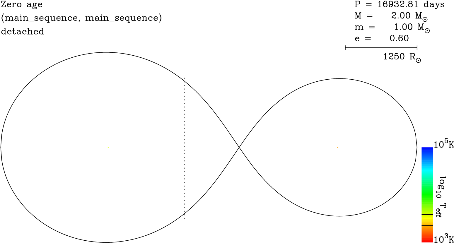
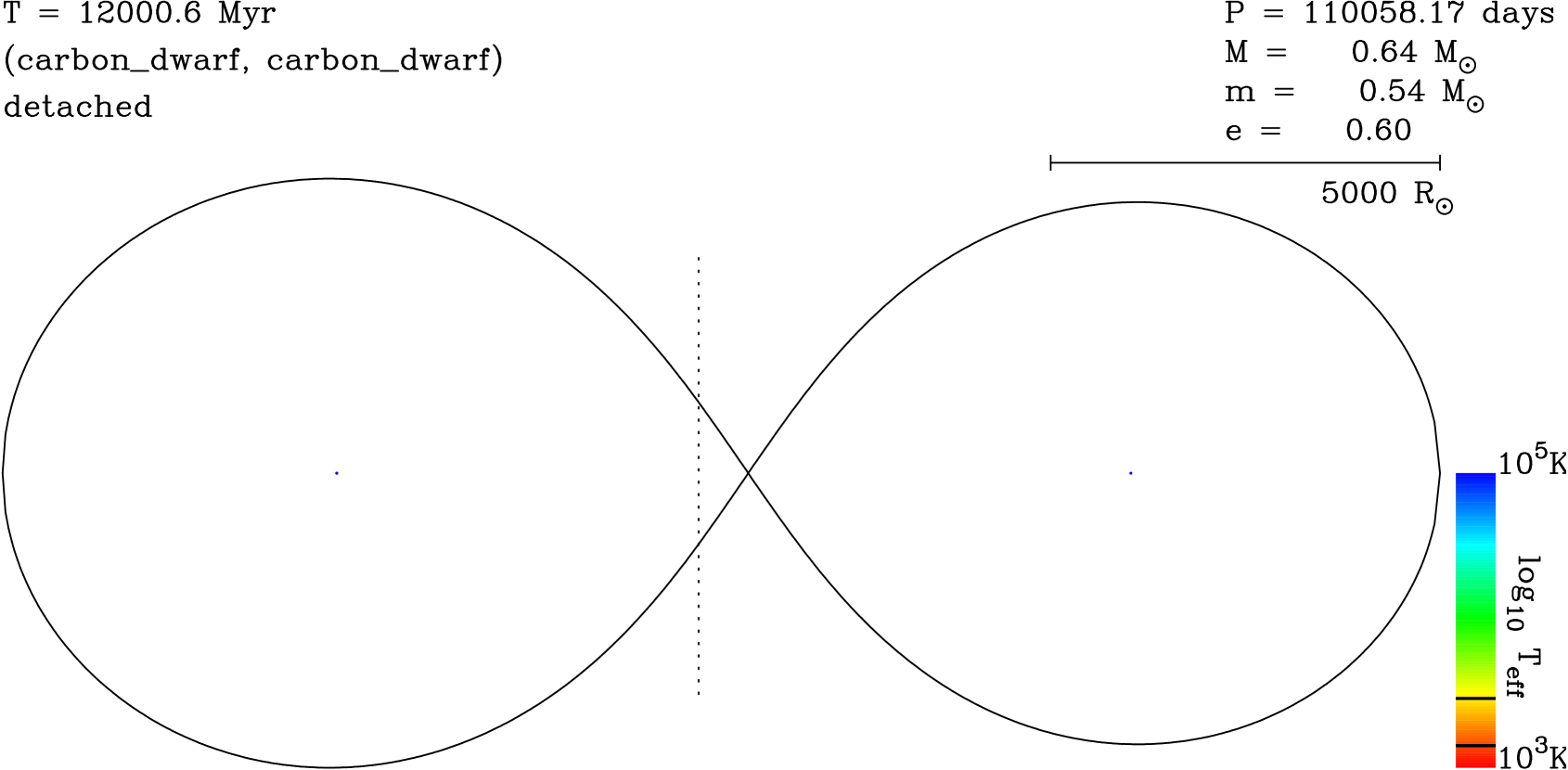
Figure 4: First and and last instance of the binary as it would evolve in isolation. Roche-lobe overflow does not occur because the binary is far too wide. Most of the legend is self-explanatory. The centre of mass lies on the vertical line. The stars in their Roche-lobes are printed to scale, rendering the main-sequence stars and white dwarfs hardly visible. The vertical shaded bar to the lower right gives an indication of the effective temperature of the stars.

The possibility of dynamical encounters makes the output considerably more interesting and also more complicated. The output of McScatter can be read by Roche, and an example is presented in fig. 5.

McScatter does not compute the orbits of 3-body encounters, and Roche is therefore not able to draw interesting spaghetti diagrams as presented in Fig.19.2 of Heggie & Hut (2003). Instead of this Roche reports strong encounters as text, as in fig. 5.

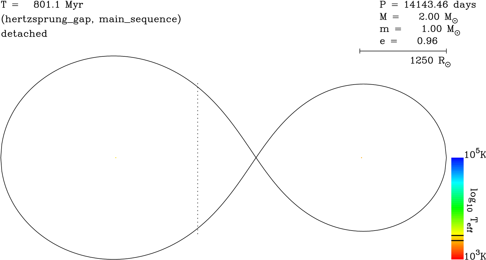
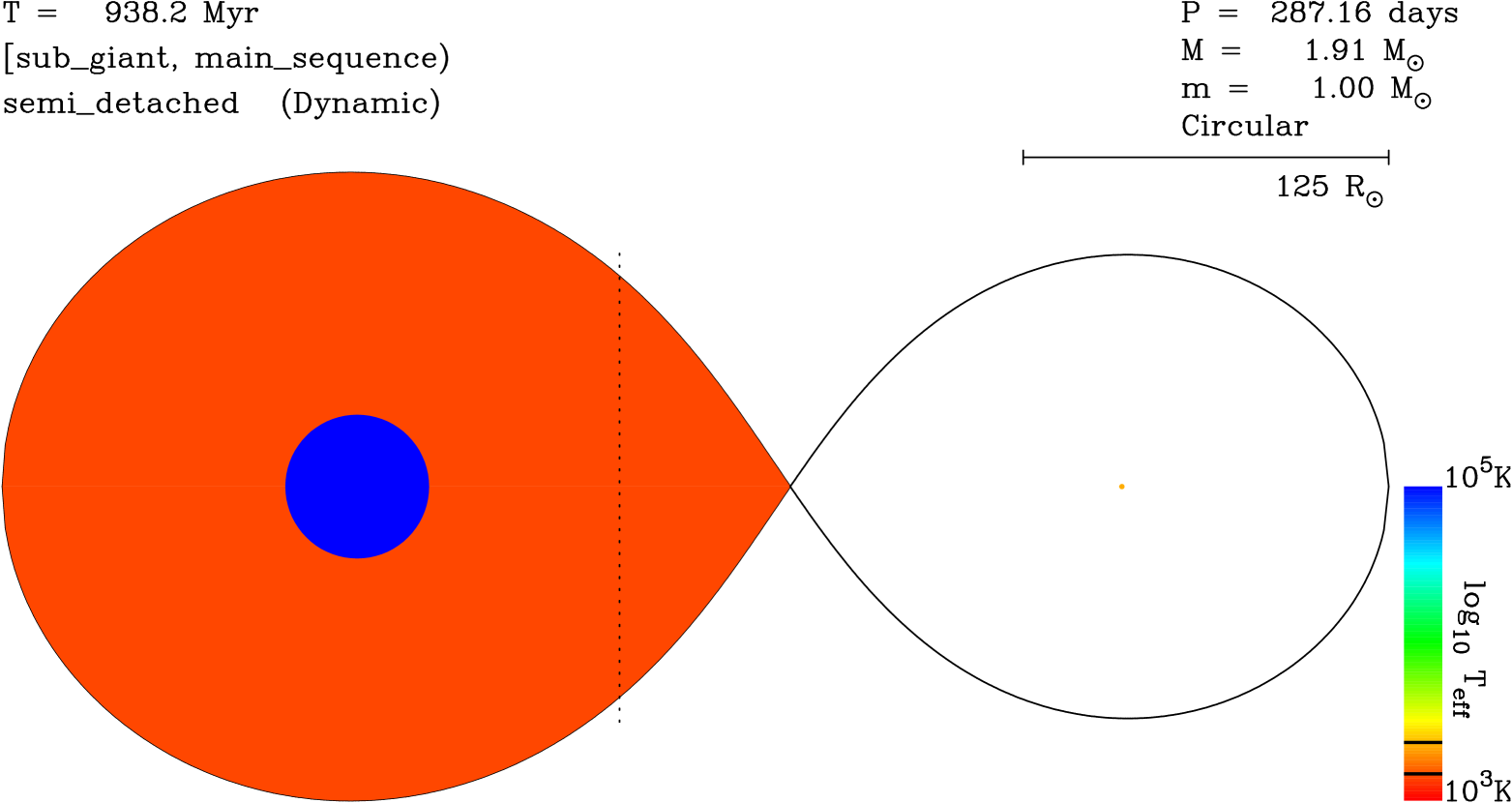
Figure 5: Evolution of the same binary is in fig. 4 in a stellar system with a density of $n=2000$ stars pc^-3. The following sequence of events occurs. Here Roche-lobe overflow occurs because the encounter with a low mass star at $t\sim 571$ Myr induces a high eccentricity on the binary. Subsequent tidal interactions circularize the binary and the orbit shrinks. The first phase of mass transfer occurs at $t\sim 938$ Myr, followed by a second phase of mass transfer at $t\sim 9.7$ Gyr (continued on the next page).

4 Conclusions

This paper presents an interface between stellar dynamics and stellar evolution which is intended for use in the context of dense stellar systems. For purposes of illustration, however, we have presented it in a situation where the dynamics is as simple as possible, i.e. a simplified model for three-body scattering between a binary and a single star. In particular, this illustrates how the interface operates even in situations where exchanges take place. The resulting toy code is called McScatter, for Monte Carlo Scattering.

To illustrate the power of our interface, we have implemented it for two independent models for the internal evolution of binary and single stars. These are SeBa, the stellar evolution package within starlab (see Portegies Zwart et al 2001), and BSE (Hurley, Tout & Pols 2002), which is usually used in conjunction with Aarseth’s N-body codes (Aarseth, 2004). These codes as they stand are not able to model such rich systems as massive globular clusters or galactic nuclei, but it is intended that our interface will be employed in other stellar dynamics codes (such as Monte Carlo codes) which can.

To highlight the differences which can arise, we have considered the scattering of a binary within a field of single stars. We have shown that the different treatment of tidal effects in the two stellar evolution packages can lead to substantial differences in the dynamical evolution of a binary. While our application is highly simplified, there is no doubt that comparable differences would arise in realistic situations.

Appendix

Here we list the basic interface routines for stellar evolution and stellar dynamics.

A     SeBa

As in starlab the stellar dynamics is supposedly the driver for the slaved stellar evolution. To assure two-way communication there is a separate set of routines to force the dynamics to update the stellar evolution, or to inform the dynamics of the state of a star or binary.

There are five families of routines, initialization, get- and set- operators, the core evolution routines, I/O routines and a miscellaneous group. The routine names start with a few characters which identify the class to which the routine belongs. These classes are: init_, get_, set_, ev_ and put_.

List of routines

• init: Initialization routines
  void init_stars(int *n, int id[], real mass[])
  void init_binaries(int *n, int id[], real sma[], real ecc[], real mprim[], real msec[])
  initialization of a list of n stars or binaries identified with arrays of length $n$ for the identity id and zero age mass mass, or in the case of a binary with primary mass mprim, secondary mass msec, the semi-major axis sma and the eccentricity ecc.

• get/set: operators to initialize and inquire the value which is identified in the second part of the function name. These routines are called for each individual star or binary separately.
  void get_mass(int *id, real *mass)
  function reads the mass from the stellar evolution package to be used in the dynamics code.
  void set_sma(int *id, real *sma)
  function initializes the orbital separation of a binary after it was affected by a strong encounter.
  Other available functions are: set/get_sma(...), set/get_ecc(...), get_radius(...), get_ss_type(...), get_bs_type(...), get_loid(...), get_hiid(...), get_loid_mass(...), get_hiid_mass(...), get_ss_updatetime(...), get_bsi_updatetime(...).
  For some parameters set_ operations are not externally available. Note that get_loid/_hiid are available to prevent confusion of the identity of the primary and secondary stars (which may or may not be the stars of lower or higher id).

• ev: routines to force evolution
  void ev_stars(int *n, int *id, real *time)
  void ev_binaries(int *n, int *id, real *time)
  Forces a list of $n$ _stars/_binaries to evolve to time *time.
  

• put: input/output routines.
  The current implementation contains only output routines:
  void out_star(int *id),
  void out_binary(int *id) and
  void out_scatter(int *idb, int *idt, real *time, bool *write_text)

• other] non-classified routines.
  void binary_exists(int *id, int *exit)
  void morph_binary(int *idb, int *idt, real *a_factor, real *ecc, int *outcome)
  function to reinitialise the binary after an exchange.

Some routines are available in plural form by adding a s to the end of the function name, these operate on arrays of stars of binaries rather than on an individual object.

B.      BSE

The routines for single- and binary-star evolution are contained in a precompiled library of Fortran subroutines and functions: libstr.a . At present versions are available for OSX, Linux PC and alpha. These are accessed through an interface, which replaces the SeBa  interface described in the previous subsection.

List of subroutines

• evStar, evBinary: These subroutines provide the link between the main program and the SSE/BSE library (or module). These routines evolve the star (or binary) forward by a user specified interval. The library routines return a recommended update timestep based on the evolution stage of the star, and the parameters dmmax (maximum allowed change in mass) and drmax (maximum allowed change in radius). The main program may or may not utilise this timestep. (This routine also produces some of the output which can be read directly by Roche.)

• initPar: Input options for the SSE/BSE library are set in this subroutine, and these may be modified by the user (see the routine for an explanation of these options). The common blocks that convey these options to the library are declared in const_bse.h.

• initStar, initBinary: These are used to initialise single stars and binaries (respectively). initBinary in turn initializes two single stars.

• ssupdatetime: Provides next update time for star i

• bsupdatetime: Calls ssupdatetime using index of primary star

• binaryexists: Determines if binary remains bound based on the index of binary type

• getLabel: Text label associated with index of stellar type

• getLabelb: Text label associated with index of binary type

• printstar: Formatted output for a single star

• printbinary: Formatted output for a binary

• print_roche_data: Primary output for the Roche package

The quantities and units used in BSE are explained in the preamble of the file interface_bse.f. In summary there are, as in SeBa, routines for setting and fetching such variable as the mass and radii of the stars and other parameters for the binary. The arrays that store these quantities are declared in interface_bse.h (where the user may choose to alter the size of these arrays, i.e. nmax). An additional file const_bse.h contains parameters needed by the BSE subroutine library.

References

Aarseth S.J., 2004. Gravitational $N$-Body Simulations. Tools and Algorithms (CUP, Cambridge)

Eggleton P.P., Fitchett M., Tout C.A., 1989, ApJ, 347, 998

Heggie D.C., Hut P., 2003. The Gravitational Million-Body Problem (CUP, Cambridge)

Heggie D.C., Hut P., McMillan S.L., 1996, ApJ, 467, 359

Hurley J. R., Pols O.R., Tout C. A., 2000, MNRAS, 315, 543

Hurley J. R., Tout C. A., Pols,O.R., 2002, MNRAS, 329, 897

Ivanova N.S., Belczynski K., Fregeau J.M., Rasio F.A., 2004, MNRAS, 358, 572

Portegies Zwart S.F., Hut, P., McMillan S.L.W., Verbunt, F., 1997, A&A, 328, 143

Portegies Zwart S.F., McMillan S.L.W., Hut P., Makino J., 2001, MNRAS, 321, 199

Spitzer L., Jr., 1987. Dynamical Evolution of Globular Clusters (PUP, Princeton)