The properties of the “standard” type Ic supernova 1994I from spectral models

Abstract

The properties of the type Ic supernova SN 1994I are re-investigated. This object is often referred to as a “standard SN Ic” although it exhibited an extremely fast light curve and unusually blue early-time spectra. In addition, the observations were affected by significant dust extinction. A series of spectral models are computed based on the explosion model CO21 (Iwamoto et al. 1994) using a Monte Carlo transport spectral synthesis code. Overall the density structure and abundances of the explosion model are able to reproduce the photospheric spectra well. Reddening is estimated to be $E(B\!-\!V)=0.30\,$mag, a lower value than previously proposed. A model of the nebular spectrum of SN 1994I points toward a slightly larger ejecta mass than that of CO21. The photospheric spectra show a large abundance of iron-group elements at early epochs, indicating that mixing within the ejecta must have been significant. We present an improved light curve model which also requires the presence of ${}^{56}\rm{Ni}$ in the outer layers of the ejecta.

1 Introduction

With the proposed connection between core-collapse supernovae of type Ic (SNe Ic) and long-duration gamma-ray bursts (GRBs; see Piran 1999 for a review), interest in SNe Ic has recently increased. The proposed picture of SNe Ic is the collapse of the core of a massive star which shed its hydrogen and helium envelope prior to the explosion. In contrast to type Ia supernovae, core-collapse supernovae exhibit a very diverse appearance. The sub-class of type Ic supernovae which have been occasionally connected to GRBs are characterised by large kinetic energies in their ejecta and are often referred to as “hypernovae” or broad-lined supernovae. The progenitors of this class of objects are proposed to be very massive stars with masses above $25M_{\odot}$ and are likely to form black holes after their collapse, while SNe Ic originating from lower mass stars probably leave a neutron star behind (e.g., Nomoto & Umeda, 2002).

In order to understand the properties of SNe Ic in general and how “normal” SNe Ic relate to the class of “hypernovae,” a systematic analysis of well-observed objects is needed. SN 1994I is regarded as a prototypical SN Ic. It has extensive observational coverage (Yokoo et al., 1994; Filippenko et al., 1995; Richmond et al., 1996; Clocchiatti et al., 1996), and it has been the subject of various theoretical studies. Both synthetic light curves and spectra have been published previously (Nomoto et al., 1994; Iwamoto et al., 1994; Baron et al., 1996; Millard et al., 1999; Baron et al., 1999); however, so far no consistent picture of the properties of this object has emerged.

SN 1994I is also important because it seems to represent the branching point of the model sequence of core-collapse supernovae proposed by Nomoto et al. (2003). Therefore, it could provide the key for a more systematic understanding of the evolution of the progenitors of the various flavours of core-collapse supernovae.

Iwamoto et al. (1994) used a low-mass model (CO21) to fit the light curve of SN 1994I. Their model has only $\sim\!1M_{\odot}$ of CO-rich ejecta, suggesting that SN 1994I was the stripped C-O core with a mass of $\sim\!2.1M_{\odot}$ originating from a $\sim\!4M_{\odot}$ He-core. This corresponds to a star with a main sequence mass of $\sim\!15M_{\odot}$. To achieve such a thorough stripping, repeated interaction with a binary companion must be envisaged.

In this work we present a series of spectral models for the early-time spectra of SN 1994I based on the explosion model CO21 by Iwamoto et al. (1994); see also Nomoto et al. (1994). This explosion model provided an excellent fit to the light curves of SN 1994I. However, light curve models alone are not able to constrain the explosion parameters uniquely because the light curve shape depends on a combination of kinetic energy and ejecta mass. The peak luminosity is constrained by the amount of ${}^{56}\rm{Ni}$ synthesised during the explosion. To determine the total luminosity, it is necessary to have reliable values for parameters such as reddening and distance. In addition, the bolometric correction used to infer the luminosity has to be derived from the shape of the spectral energy distribution. Using the highly parametrized spectral code SYNOW (Fisher et al., 1999, and references therein), Millard et al. (1999) provided line identifications for some of the spectra of SN 1994I. Baron et al. (1999) have calculated non-local-thermodynamic equilibrium (non-LTE) models for a few spectra based on the outcome of CO21 and concluded that this model is not able to reproduce the observed spectra in detail. They suggested that a higher mass model would be required to match the line features better.

2 Spectral models

We used the observed spectra published by Filippenko et al. (1995) which have been flux calibrated against the photometry of Richmond et al. (1996). Our series of photospheric models covers the observations from April 4 to May 4, 1994. (UT dates are used throughout this paper.) For all models the explosion date was set to be March 27, 1994 (JD 2 449 439), corresponding to a rise time to $B$-band maximum of $12\,$d (Iwamoto et al., 1994). In what follows the epochs are given in days relative to this date. The $B$-band maximum of SN 1994I occurred on April 7 (JD 2 449 450) (Richmond et al., 1996). We have excluded the first spectrum (April 2) in Filippenko et al. (1995) because the wavelength coverage of this observation is too narrow for a conclusive model. Spectra later than May 5 already show too much nebular emission to be treated with a photospheric approach. In addition, we used a spectrum from April 3 that was taken at the Multiple Mirror Telescope (MMT) by Schmidt et al. (1994, priv. comm.).

The early-time spectral models have been computed employing the method which was first proposed by Abbott & Lucy (1985) and further developed by Mazzali & Lucy (1993), Lucy (1999), and Mazzali (2000). The method employs a Monte Carlo simulation of the line transfer based on the Sobolev approximation and includes a line-branching scheme. At the end of the Monte Carlo calculation the emergent spectrum is derived from a formal integral solution on the basis of the source functions that can be extracted from the Monte Carlo simulation (see Lucy, 1999).

For the model computation the ejected material is divided into an outer region, where the true continuum opacity is assumed to be negligible, and an inner region which is not treated explicitly. At the dividing boundary of the computational area a thermal blackbody continuum is imposed with a temperature that is adjusted according to the luminosity of the emergent radiation at the outer boundary. Note that this temperature has to be determined in an iterative process because it is a priory not clear what fraction of the radiation is scattered back into the core region. This constitutes the effect of line blanketing where the back-scattered radiation causes the matter to heat up. The ejecta are treated in spherical symmetry. At this stage we assume a homogenised composition for the entire computational volume.

To fit the early-time spectra we used the density structure from the CO21 explosion model (Nomoto et al., 1994; Iwamoto et al., 1994). The model is expanded homologously to match the desired epoch. The composition was adjusted in order to obtain a good fit to the observed spectrum. The abundance distribution from the nucleosynthetic yields of the CO21 model averaged over velocity space above each epoch’s photosphere served as a guideline. We adopt a distance to the host galaxy of $8.4\,$Mpc, corresponding to a distance modulus of $\mu=29.6\,$mag (Feldmeier et al., 1997).

2.1 Reddening

The amount of extinction by dust has a significant impact on the estimate of the total luminosity of the object and, therefore, the amount of synthesised ${}^{56}\rm{Ni}$ derived from models. The extinction toward SN 1994I has been a controversial topic (Baron et al., 1996; Richmond et al., 1996) and could not be firmly established. The presence of a strong, narrow Na i D line in the spectra, as well as the colours, suggest that the object was significantly reddened, but the exact amount is subject to large uncertainty. While the analysis of the Na i D line implies a very large extinction of $E(B\!-\!V)\approx 1$ (Ho & Filippenko, 1995), spectral models by Baron et al. (1996) suggest a value for $E(B\!-\!V)$ between $0.30$ and $0.45\,$mag.

The amount of reddening affects the model spectra because the luminosity affects the temperature and hence the properties of the spectrum (given a fixed distance and density structure). The temperature structure determines the overall shape of the spectrum and, via the ionisation balance, the strengths of characteristic line features. A test series of different values for $E(B\!-\!V)$ between $0.15$ and $0.50\,$mag showed a preferred range between $0.25$ and $0.35\,$mag. For larger reddening the ionisation tends to be too high to reproduce the characteristic lines of singly ionised species (Millard et al., 1999). A value of $E(B\!-\!V)$ near the lower end results in temperatures that shift the line ratios, in particular those of Ca ii, too much toward the transitions with low excitation energies. For our full series we chose $E(B\!-\!V)=0.30\,$mag, however note that the uncertainty for this value may be as large as $\pm 0.05\,$mag. For models with larger reddening the composition required to fit a spectrum contains more iron-group elements at the expense of lighter elements because a larger reddening requires a larger temperature, shifting the spectrum to the blue. This blue-shift has to be counterbalanced by stronger line blocking, which is efficiently provided only by iron-group elements having a large number of lines.

In the following the properties of each model are briefly discussed.

2.2 Model series for the photospheric epoch

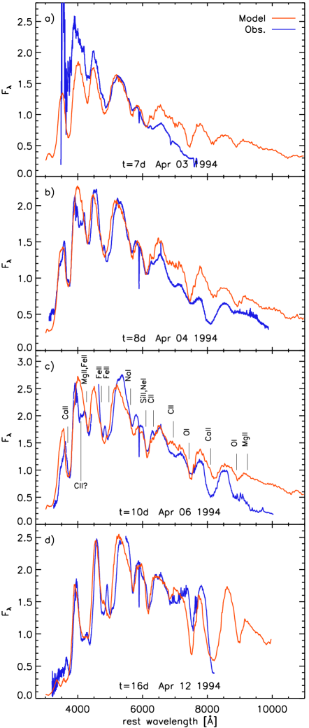
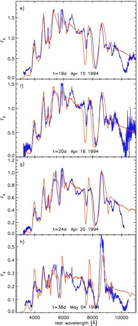
Figure 1: Synthetic spectra of SN 1994I in comparison with the observed spectra. The observations are from Filippenko et al. (1995), except for the spectrum of April 3, which was taken at the MMT (Schmidt et al. 1994, priv. comm.). For each spectrum the epoch in days after the assumed explosion date (March 27, 1994) is indicated. The flux $F_{\lambda}$ is given in units of $10^{-14}\,$erg cm^-2 s^-1 Ź. In panel c the ions that form the major contribution to the observed features are indicated. The identifications do not change significantly at different epochs.

2.2.1 $t=7\,$d, April 3, 1994

For this spectrum the calibration against the corresponding photometry required a correction of $0.17\,$mag to match the $R$ and $V$ bands reasonably well. However, with this correction the $U$ and $B$ bands are still too bright by $0.67$ and $0.30\,$mag, respectively. This deviation is too large to apply a single averaged value. Therefore we re-calibrated the spectrum to match only the $V$ and $R$ bands, which represent the majority of the flux. Keeping this inconsistency in mind, we did not try to match the observations exactly but rather adjusted the model to obtain the basic features and reach agreement with the $U$, $B$, $V$ and $R$ photometric points for this epoch. Consequently, the fit does not look too good at all wavelengths (see Fig. 1a), but the main features are reproduced, except for the O i $\lambda 7774$ line, which is significantly weaker in the observed spectrum. This line tends to be too strong in all our models. It is a highly saturated line that is fairly insensitive to changes in the oxygen abundance, within reasonable limits.

Apart from the inconsistency in the data, part of the problems to fit the overall slope of the observed spectrum could also arise from the model assumption of a thermal lower boundary which may not sufficiently represent the physical conditions in the ejecta. We discuss this possibility in Sec. 3.2.

2.2.2 $t=8\,$d, April 4, 1994

The total luminosity required for this model is $L=1.89\times 10^{42}\,$$\rm{erg\,s}^{-1}$. With a photospheric velocity of $v_{\rm ph}=11\,600\,$$\rm{km\,s}^{-1}$ this results in a temperature of the underlying blackbody of $T_{\rm BB}=9679\,$K. In the blue and visible wavelength bands the fit is reasonable, while the slope of the pseudo-continuum of the model does not match that observed in the redder parts of the spectrum. The spectrum shows various strong absorption features which can be attributed to the ions indicated in Fig.1c. Interestingly, the absorption at $\sim\!6100\,$Å is only partially produced by Si ii; it also contains a significant contribution from various Ne i lines, most important Ne i $6402$. As before, the absorption feature of the O i $\lambda 7774$ line appears too deep.

The model also does not reproduce the spectral slope of the observation redward of about $6500\,$Å. Part of this problem may, as in the previous spectrum, be due to a calibration problem in the data. The correction that was applied to match the $V$ and $R$ photometry results in an offset of $0.14\,$mag in the $I$ band. Therefore, the $I$-band magnitude of the model is actually in closer agreement with the photometry than the integrated magnitude of the spectrum in that bandpass filter. Nevertheless, also for this case the possibility of a physical effect that is not correctly represented in the model should be kept in mind (see Sec. 3.2).

Another interesting feature of this spectrum is the absorption structure between $4000\,$Å and $4200\,$Å which Millard et al. (1999) attribute to Sc ii. In our models we can reproduce that feature using significant amounts of Sc, but this also causes a variety of other Sc lines to show up elsewhere in the spectrum. In the later spectra the observed absorption seems to grow into a distinct feature which is mostly caused by Ti ii and Fe ii lines, while there is no clear indication for Sc lines anymore. Therefore we suggest that even in the early spectrum the main components of this feature are Fe lines that are not correctly reproduced by our model. In addition, other ions such as C ii and Si ii contribute to this feature to some extent.

2.2.3 $t=10\,$d, April 6, 1994

This spectrum (Fig. 1c) represents the observation closest to the $B$-band maximum, which occurred on April 7 (Richmond et al., 1996). In this model, the continuum slope is already better reproduced than in the first spectra although there is still an offset redward of $\sim\!7000\,$Å. We used a photospheric velocity of $v_{\rm ph}=10\,800\,$$\rm{km\,s}^{-1}$. The total luminosity increased to $L=2.31\times 10^{42}\,$$\rm{erg\,s}^{-1}$, and the temperature of the incident radiation was $T_{\rm BB}=9230\,$K. With the exception of the “Sc” feature and red continuum slope, the fit is reasonably good. The observation starts to show the separation of the Fe ii feature at $4900\,$Å which is reproduced by the model at this epoch. Also, the depth of the Ca ii infrared lines is not sufficient in the model while the Ca ii H&K absorption is fitted well.

2.2.4 $t=16\,$d, April 12, 1994

This spectrum (Fig. 1d), $16\,$d after explosion (corresponding to $5\,$d after $B$-maximum), exhibits clear differences compared to the pre-maximum spectra, and it is significantly redder. The parameters that have been used for this fit are $L=2.10\times 10^{42}\,$$\rm{erg\,s}^{-1}$ for the total luminosity and a photospheric velocity of $v_{\rm ph}=8800\,$$\rm{km\,s}^{-1}$. The resulting temperature at the inner boundary was $T_{\rm BB}=7690\,$K. The double structure between $4500\,$ and $5000\,$Å is more pronounced, and our model mostly fails to reproduce it. The feature is mainly formed by Fe ii lines that are all part of the same multiplet (Fe ii $\lambda\lambda 4923,5018,5169$). The fact that we see the lines separated in the observation indicates that either the density or at least the ionisation fraction of Fe ii must have a steep gradient in the velocity region just above the photosphere, which is not reproduced by our models of the earlier epochs. At later epochs the models resolve this structure better.

Apart from that, most of the features in the model are systematically blue-shifted compared to the observation. Even with a drastic change of parameters this problem remained, suggesting that the density structure is too flat within the velocity range where most lines form at this epoch.

2.2.5 $t=19\,$d, April 15, 1994

The luminosity used for this model (see Fig. 1e) decreased further to $L=1.46\times 10^{42}\,$$\rm{erg\,s}^{-1}$ at a photosphere located at $v_{\rm ph}=7200\,$$\rm{km\,s}^{-1}$ with a temperature of $T_{\rm BB}=6999\,$K. In this spectrum the double feature of Fe lines below $5000\,$Å also starts to show in the synthetic spectrum.

Starting from this epoch the slope of the near-IR flux is well reproduced by the model. This may be surprising because at later epochs the approximation of a photosphere becomes less accurate. Given the compactness of model CO21, it may be that the photospheric approximation holds reasonably well even at epochs well after maximum (see §3.2).

The model does not provide clear evidence for the origin of the deep absorption observed at $10\,500\,$Å. In previous work (Filippenko et al., 1995; Clocchiatti et al., 1996; Millard et al., 1999; Baron et al., 1999), various suggestions for the origin of this feature have been discussed, but no conclusive answer could be reached. We will investigate this feature in §3.3

2.2.6 $t=20\,$d, April 16, 1994

This spectrum (Fig. 1f) is just a day after the previous one and therefore fairly similar. A model with $L=1.30\times 10^{42}\,$$\rm{erg\,s}^{-1}$, $v_{\rm ph}=6800\,$$\rm{km\,s}^{-1}$, and $T_{\rm BB}=6774\,$K reproduces most features quite well, except that some of the peaks tend to be somewhat low.

The narrow peak at $6560\,$Å, which is not reproduced by our model, could to some extent be due to emission of H$\alpha$ by a surrounding shell. To test this possibility, however, is beyond the scope of this work.

2.2.7 $t=24\,$d, April 20, 1994

The $t=24\,$d epoch represents the last of the early spectral series. Overall this spectrum is still similar to the one taken $4\,$ days earlier, except that the Fe ii and Na i lines become deeper. For the model in Fig. 1g we used $L=9.18\times 10^{41}\,$$\rm{erg\,s}^{-1}$ and a photospheric velocity of $v_{\rm ph}=5400\,$$\rm{km\,s}^{-1}$. The temperature of the photosphere was derived to be $T_{\rm BB}=6383\,$K.

2.2.8 $t=38\,$d, May 4, 1994

This spectrum, $38$ days after explosion, is already quite late to be treated with a photospheric code because it may contain a significant fraction of nebular-line emission mixed into the emission components of the P-Cygni profiles. Therefore, it is not surprising that some of the emission features cannot be reproduced by this approach (e.g., the Ca ii IR triplet). Nevertheless, the fit is reasonable (see Fig. 1h). The luminosity used was $L=3.49\times 10^{41}\,$$\rm{erg\,s}^{-1}$; the photosphere was set to $v_{\rm ph}=2100\,$$\rm{km\,s}^{-1}$. These values are not strongly constrained because a clear definition of a photosphere is not possible at such late epochs. Rather, the velocity sets the radius which is required to obtain the correct temperature structure to reproduce the correct ionisation ratios given the chosen luminosity. The temperature at the photosphere was $T_{\rm BB}=6129\,$K.

2.3 Nebular Spectrum, $\mn@boldsymbol{t=159}\,$d

As is typical for SNe Ic, the nebular phase develops early because of the small ejecta mass. To test the inner part of the ejecta we also modelled the nebular spectrum taken on September 2 using a non-LTE nebular code (Mazzali et al., 2001) which assumes a constant density, one-zone model inside a given velocity.

Figure 2: Nebular model for the nebular spectrum $159\,$d after explosion compared to the observation assuming a reddening of $E(B\!-\!V)=0.30\,$mag. $F_{\lambda}$ is in units of $10^{-15}\,$erg cm^-2 s^-1 Ź

The spectrum has an epoch of $159\,$d after the proposed explosion date. It was corrected based on the photometric data of Richmond et al. (1996) but in the blue part the correction is somewhat uncertain because of the presence of an underlying galaxy continuum. However, this uncertainty does not significantly affect the conclusions in this section.

For the model shown in Fig. 2 we assumed an expansion velocity of $v_{\rm exp}=5500\,$$\rm{km\,s}^{-1}$ at an epoch of $t=159\,$d. The model has a mass of $M=0.43{M_{\odot}}$ below this velocity. To reproduce the correct line strengths using the same distance and reddening values as for the photospheric spectral series, $0.07M_{\odot}$ of ${}^{56}\rm{Ni}$ are required. This generates a luminosity of the nebula of $L=2.22\times 10^{40}\,$$\rm{erg\,s}^{-1}$ with a faction of $\sim\!10\,$per cent of the $\gamma$-rays depositing their energy in the gas. The remaining composition needed to reproduce the spectrum includes $0.22M_{\odot}$ oxygen, $0.09\,M_{\odot}$ carbon, $0.02M_{\odot}$ silicon, and $0.02M_{\odot}$ sulphur.

Table 1: Nebular models for different values of reddening.

$E(B\!-\!V)$ [mag]	$0.15$	$0.30$	$0.45$
$M_{\rm total}$ [$M_{\sun}$]	$0.36$	$0.43$	$0.54$
$M(^{56}\rm{Ni})$ [$M_{\sun}$]	$0.05$	$0.07$	$0.09$
$M({\rm O})$ [$M_{\sun}$]	$0.18$	$0.22$	$0.28$
$L_{\rm dep}$ [$10^{40}\,$$\rm{erg\,s}^{-1}$]	$1.42$	$2.22$	$3.31$

To test the impact of reddening we calculated a series of models with different values for $E(B\!-\!V)$: $0.15$, $0.30$, and $0.45\,$mag. Within this range of $E(B\!-\!V)$ it is possible to find a set of parameters that fit the observed spectrum well, but the masses of the various models are different. The resulting parameters for these models are summarised in Table 1.

The mass enclosed within $5500\,\rm{km\,s}^{-1}$ is larger than the corresponding mass of CO21, which is only $0.1M_{\odot}$. Also, the line profiles do not suggest the presence of a mass cut at a velocity of $\sim\!2000\,\rm{km\,s}^{-1}$ but indicate the presence of material at lower velocities.

3 Discussion

3.1 Composition and derived magnitudes

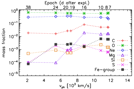
Figure 3: Mass fraction of the various elements versus the velocity of the photosphere ($v_{\rm ph}$) that was used for the respective model. At each epoch the models are calculated assuming a homogeneous distribution of the elements.

Fig. 3 shows a plot of the mass fraction for some elements used for the respective models versus the photospheric velocity, $v_{\rm ph}$. Note that we assume a homogeneous composition for each model; hence, this plot will only roughly represent a slice of the ejecta composition. In particular, for features that form significantly above the photosphere, the velocity may not be representative. Also, for elements that do not contribute any distinct line features, the abundance is not strongly constrained.

An interesting aspect of this plot is that the abundance of iron-group elements (Ti, Cr, Fe, Co, and Ni) decreases toward lower photospheric velocities. This is a feature which is seen in hypernovae that exhibit strong jet-like asymmetries. The fact that we find a higher concentration of heavier elements in the outer part of SN 1994I may suggest that the explosion of this object also showed asymmetry to some extent, although the nebular spectra do not show a strong indication for that.

In comparison to the original CO21 model, we get a significantly larger mass fraction of oxygen at low velocities at the expense of iron-group elements. The high abundance of iron-group elements at velocities above $\sim\!7000\,\rm{km\,s}^{-1}$ is also not predicted by CO21 even if we assume some contribution of primordial material with solar composition added into the outer part of the explosion model. The abundance of Si is significantly lower than predicted by CO21, while C and Ne seem to be more abundant. On the basis of the spectral models it is not possible to put strong constraints on the detailed composition structure; in particular, for elements that do not have many spectral lines, the error bars may be quite large. Nevertheless, there is strong indication that the composition is more strongly mixed than in the theoretical ejecta model.

Fig. 4 shows the magnitudes derived from the models in comparison to the “observed” magnitudes. The data points for $B$, $V$, and $R$ have been obtained by interpolating the original points of Richmond et al. (1996) to the epochs of the corresponding spectral observations. The $U$-band points are taken from Schmidt, et al. (1994, priv. comm.) and are shown at the original epochs because there is insufficient spectral coverage of this wavelength band. Since the models resemble the observed spectral shapes reasonably well, the magnitudes from the models are overall in good agreement with the observed ones. Only at the later epochs the $U$-band magnitudes are underestimated by the models.

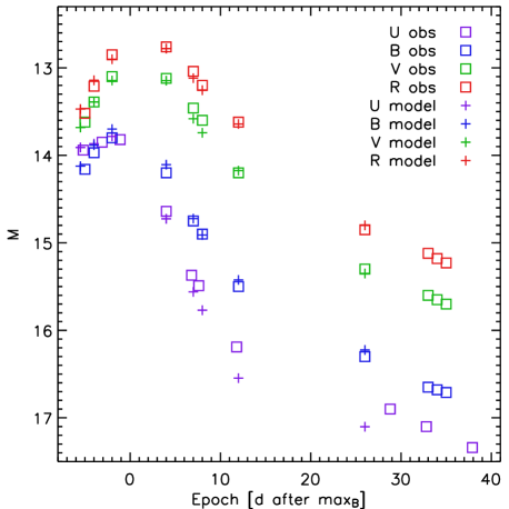
Figure 4: Comparison of observed (squares) and model (crosses) magnitudes in different wavelength bands. The observed magnitudes for $B$, $V$, and $R$ have been obtained by interpolating the photometry points from Richmond et al. (1996) to the observation dates of the spectra. The $U$-band points are from Schmidt, et al. (1994, priv. comm.).

3.2 The location of the “photosphere”

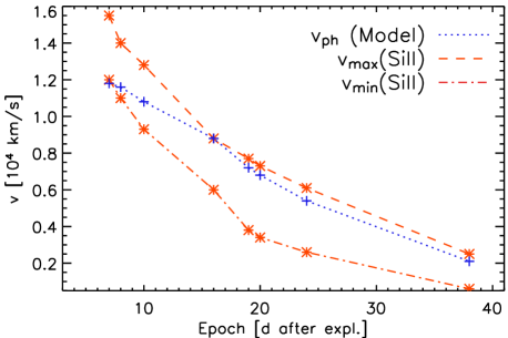
Figure 5: Photospheric velocities of the models as a function of epoch in comparison to the velocities measured from the “Si ii” feature at $6100\,$Å (see text).

Fig. 5 shows the photospheric velocities ($v_{\rm ph}$) derived from the models as a function of epoch. Also indicated are the measurements of the line velocity from the observed spectra assuming that the $\lambda 6100$ feature is due to Si ii$\,6347,6372$. Our models suggest that there may be a significant contribution from Ne i $6402$. This would result in an underestimate of the “real” velocity because the Ne i line has a slightly redder rest wavelength. The upper and lower limits correspond to different assumptions on the blend of lines that makes this feature. The lower dotted curve corresponds to a fit to the feature with a single Gaussian profile, while the upper dotted curve represents the estimate from a fit with two Gaussian profiles assuming that the bluer one is Si ii. At the early epochs the photospheric velocities of the models clearly exhibit a different trend. Therefore, the absolute velocities deduced in this way may not be a good representation of the photospheric velocities and should not be over-interpreted.

Because the photospheric velocity of the models are primarily constrained by the temperature that is needed to match the shape of the spectrum and the degree of ionisation, this different behaviour of the Si ii velocities may result from the failure of the approximation to describe the shape of the early-time spectra with a thermal blackbody continuum. The mismatch between the observed and model red continua give another indication that this description is not appropriate for those epochs. Generally, in hydrogen-deficient supernovae the assumption of a thermal continuum photosphere is questionable because the physical conditions present in the ejecta do not result in sufficient true continuum opacity to achieve thermalization (e.g., Sauer, 2005, Sauer et al, in prep.). Imposing this thermal continuum in the models generally leads to an offset of the model flux in the red and infrared wavelength bands.

This problem is less severe in SNe Ic than in SNe Ia because the composition by mass fraction is dominated by the lighter species (oxygen and neon) while in SNe Ia the iron-group elements make the largest contribution. This means that even for the same mass density, the number density in SNe Ic is larger by a factor of up to $2$. Since the true processes (bound-free and free-free transitions) that are needed to thermalize photons scale with the number density of the ions and free electrons, the processes are more effective in SNe Ic. In addition, the stronger influence of Thomson scattering (which is also proportional to $n_{e}$) will result in a larger number of scattering events for each photon before it can escape the ejecta. This effectively increases the volume in which the photons have a chance of being thermalized. This may explain why the spectral shape of SN1c spectra can be described fairly well with a thermal continuum to later times whereas in SNe Ia, the approximation to assume a blackbody continuum at the photosphere becomes increasingly worse for later times.

The early-time spectra of SN 1994I are very blue suggesting that they may have a stronger component of non-thermalized radiation than the later ones. This may be due to a steep gradient in the density in the outer parts of the ejecta. If a substantial quantity of $\gamma$-ray photons is generated in the outer, thinner layers of the ejecta, the effective path lengths of the photons may become too short to allow the photons to be thermalized. A prerequisite for the presence of a non-thermalized radiation field at early times is, however, a significant amount of radioactive ${}^{56}\rm{Ni}$ located in the outermost layers of the ejecta. This outer layer of Ni would not strongly contribute to the later light curve, as a large fraction of the $\gamma$-ray photons would escape without depositing their energy in the ejecta. Some ${}^{56}\rm{Ni}$ is indeed needed in the outer part of the ejecta to reproduce the early light curve rise (see §4)

For a more consistent investigation of this phenomenon a better description that includes the non-thermal formation of the pseudo-continuum is needed.

3.3 The infrared feature at 10 300 Å

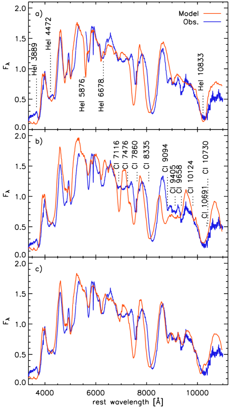
Figure 6: Models for the $t=19\,$d spectrum. In the upper panel (a) the strength of the helium lines was artificially enhanced above $v\approx 16\,000\,\rm{km\,s}^{-1}$ by factors between $10^{8}$ and $10^{12}$ to mimic non-thermal excitation in an outer helium-rich shell (assuming a homogeneous mass fraction of $10.5$ per cent for helium). It is not possible to reproduce the broad absorption feature at $10\,300\,$Å in this way without also increasing the strength of the He i $\lambda 5876$ line to a level that is not observed. The labels in Panel a indicate the positions of the strongest He i lines at a velocity of $v_{\rm He}=17\,000\,$$\rm{km\,s}^{-1}$. The middle panel (b) shows a model obtained by increasing the optical depth in the C i line by factors of $10^{3}$ to $2\times 10^{3}$ above $14\,000\,$$\rm{km\,s}^{-1}$ to fit the $10\,300\,$Å absorption. The mass fraction of carbon was $21.7$ per cent. This model shows a variety of C i lines in other places that are not observed. The positions of the C i lines correspond to a velocity of $v_{\rm C}=9000\,\rm{km\,s}^{-1}$. The lower panel (c) shows a model with both He i and C i enhanced. The enhancement factor for He i above $16\,600\,$$\rm{km\,s}^{-1}$ reaches from $10^{9}$ to $10^{12}$, for C i we applied a factor of $50$ in the entire ejecta. This leads to an acceptable fit of not only the IR-absorption but also various other lines at $\sim\!9000\,$Å, which are not reproduced by the original model (Fig. 1e). The flux is given in units of $10^{-14}\,$erg cm^-2 s^-1 Ź.

Spectra that extend into the near infrared (Fig. 1e-h) show a distinct and broad absorption feature around $10\,300\,$Å. Originally, this feature was attributed to He i $\lambda 10\,830$ (Filippenko et al., 1995; Clocchiatti et al., 1996). However, as pointed out by Baron et al. (1999), this identification would require a detection of at least He i $\lambda 5876$ at similar velocities ($\sim\!15\,000\,$$\rm{km\,s}^{-1}$) in the observed spectrum. To model the He i lines correctly it is necessary to consider the non-thermal excitations by fast electrons caused by Compton scattering of $\gamma$-photons from the ⁵⁶Co decay. Without those processes the excitation of He i at the temperatures present in the ejecta is too low to cause any significant absorption (Lucy, 1991).

Since our code does not treat non-thermal processes we cannot address this problem in a self-consistent way. To nevertheless test the possibility that He i causes the $10\,300\,$Å absorption we enhanced the optical depth in the He i lines introducing by hand a “non-thermal factor” that mimics the effects of departure from LTE caused by the fast electrons produced by the deposition of $\gamma$-photons (see Harkness et al., 1987; Tominaga et al., 2005). We allowed this factor to vary with velocity to obtain a good fit of the $10\,300\,$$\rm{km\,s}^{-1}$ absorption. Although some lines arise from the singlet system and others from the triplet system, such as $\lambda 6678$, we applied a single enhancement factor to all He i lines. The studies of Lucy (1991) and Mazzali & Lucy (1998) find that the departure from LTE is comparable for both states. We chose the observed spectrum of $t=19\,$d (cf. Fig. 1e) for this study because that is the earliest observation that extends far enough to the IR to show this feature. In the first model shown in Fig. 6a we enhanced the optical depth in all He i by a factor that varied from $10^{8}$ at $16\,000\,$$\rm{km\,s}^{-1}$ to $10^{12}$ in the outermost shells above $30\,000\,$$\rm{km\,s}^{-1}$. The abundance of helium was uniformly set to $10.5$ per cent by mass. Most of the strong He i lines that also show up in the model spectrum blend in with other features in the spectrum, however the model inevitably shows a clear absorption at $\sim\!5500\,$Å. $\lambda 10\,833$ is the strongest He i line in our model and thus may show up before any other lines can be clearly identified. Unfortunately, the observed spectra that cover the infrared wavelengths have a gap in the region where the He i $\lambda 5876$ lines would be expected. The observed spectra of the later epochs that do cover this wavelength range show a small absorption dip in the peak around $5450\,$Å, which could be identified with the He i $\lambda 5876$ lines, but the feature is not clearly present in the early epoch spectra. Apart from this, the observed absorption is much weaker than what the model spectrum would suggest for this line. Also, the corresponding velocity for He i would be $26\,000\,$$\rm{km\,s}^{-1}$, which is inconsistent with the identification of He i $\lambda 10\,833$ for the $\lambda 10\,300$ absorption. Of course, the method adds more free parameters and therefore the abundance of He i cannot be constrained but depends on the choice of the enhancement factor (for a given density of the explosion model). The very large enhancement factors needed to obtain a reasonable fit, however, indicate that an unreasonably large amount of several solar masses of helium would have to be present at the high velocities to obtain this absorption considering that to account for the non-thermal excitation alone should not require a factor of more than a few $10^{5}$ (Lucy, 1991; Mazzali & Lucy, 1998).

Millard et al. (1999) argue from their highly parametrized line fits with SYNOW that the $10\,300\,$Å feature could originate from a blend of He i, Si i, and C i lines. In our models of these epochs the ionisation equilibrium is generally such that Si ii is more abundant than Si i by several orders of magnitude. Therefore, the mass in Si needed to obtain considerable absorption in Si i is very high and leads to a significant overestimate of the Si ii lines in the spectra. The strongest line of Si i in the observed wavelength range is Si i $\lambda 10\,790$. If we assume that this line is primarily responsible for the observed IR absorption, it follows that the velocity of this Si i layer should be around $15\,500\,$$\rm{km\,s}^{-1}$. In that case one would also expect the presence of absorption features by the much stronger Si ii $\lambda\lambda 6241,6349$ lines but none of the spectra suggest the presence of such a high-velocity silicon layer. Given those indications, we regard the identification with Si i as unlikely.

The presence of carbon at velocities below $11\,000\,$$\rm{km\,s}^{-1}$ at day $19$ is consistent with the earlier spectra at $t=8\,$d and $10\,$d: The small features in the peak around $4100\,$Å in those early spectra (see line label in Fig. 1c) can be partially attributed to C ii $\lambda 4267$ at a velocity around $11\,000\,$$\rm{km\,s}^{-1}$, although our models do not reproduce the details of the spectrum in that region The smaller absorption features between the Ca ii IR-triplet and the deep absorption at $10\,300\,$Å in the later spectra can be identified with C i lines. These lines are indicated in Fig. 6b, which shows a model in which the optical depth in C i was enhanced above $14\,000\,\rm{km\,s}^{-1}$ by factors between $10^{3}$ and $2\times 10^{3}$ to fit the $10\,300\,$Å absorption. The mass fraction of carbon in this model is $21.7$ per cent. The positions of those lines correspond to a velocity of around $9500\,$$\rm{km\,s}^{-1}$, which also agrees with the velocity of the O i lines near $7500\,$Å. The enhancement factors needed for C i are significantly lower than for helium. In addition, the observed spectra of earlier epochs are consistent with the presence of C ii lines at similar velocities. Nevertheless, the model shown in Fig. 6b does also not provide a reasonable fit to other spectral regions. That suggests that carbon alone may also not be the cause of the $10\,300\,$Å absorption.

The lower panel in Fig. 6 shows a model with different factors mimicking non-thermal excitations in both He i and C i. This combination gives a good fit not only to the IR-absorption but also to the C i-lines shown in Fig. 6b. In addition, the amount of He i needed is low enough not to cause strong absorptions elsewhere in the spectrum. For this model the optical depth in He i was enhanced by factors between $10^{9}$ to $10^{12}$ above $16\,600\,\rm{km\,s}^{-1}$. For C i a uniform factor of $50$ was applied in the entire ejecta. The relatively small enhancement-factors needed for C i and the fact that one would not expect that non-thermal effects are significant for this ion, suggest that a slightly different composition and ionization structure at larger velocities may be responsible for the formation of the C i lines.

For a more conclusive determination the effect of varying composition as well as a more physical description of the non-thermal excitations has to be considered. Also, as pointed out by e.g. Przybilla (2005), in full non-LTE calculations of early type stars the strength of the IR-He i line sensitively depends on the correct treatment of line blocking as well as the details of the chosen model atom. Therefore, fully consistent non-LTE models will be necessary to model the formation of this line.

3.4 Oxygen abundance and total mass

Common to all synthetic fits of the photospheric epochs presented in §2is the fact that the predicted O i $\lambda 7774$ line that is too strong. This line is highly saturated and does not depend sensitively on the abundance assumed for oxygen. Therefore, one has to adopt a very low oxygen abundance to fit the observed depth of the O i line. In the $t=19\,$d spectrum, for example, the oxygen mass fraction has to be reduced to $\sim\!4$ per cent. At the same time, however, a significant oxygen mass of $0.22M_{\odot}$ is needed in the innermost region to reproduce the nebular spectrum (see §2.3).

Another possibility is that the total oxygen mass fraction is indeed larger, but that, owing to non-thermal ionisation processes the ionisation of O i is actually higher than derived by our models. O ii does not have many lines from low-lying levels in the observed wavelength bands. The presence of unexplained absorption dips in the spectra around $7000\,$Å could hint at forbidden O ii lines, which have also been suggested by Millard et al. (1999). Non-thermal ionisation can be induced by some amount of mixing of ${}^{56}\rm{Ni}$-rich material into the oxygen layers. The larger amount of oxygen in the inner region seen in the nebular phase supports this scenario.

The obvious contradiction in this picture, however, lies in the identification of C i lines in the infrared as discussed in the previous section. If C i is seen at velocities similar to that of the O i line, it is not clear why non-thermal ionisation processes should affect oxygen but not carbon.

3.5 Bolometric light curve

The bolometric light curve is one of the common ways to constrain a theoretical model. Ideally, to obtain a bolometric light curve from observed data one uses a set of well-calibrated spectra from UV through IR wavelengths. The available data for SN 1994I does not cover the $J\!H\!K$ bands in the infrared. We computed the bolometric light curve of SN 1994I using the photometric data in $U\!BV\!R\!I$ (Richmond et al. 1996 and B. Schmidt, priv. comm.). This $U\!BV\!R\!I$ integrated light curve from SN 1994I data (open squares in Fig. 7) alone represents a lower limit to the bolometric light curve since the IR contribution is not taken into account.

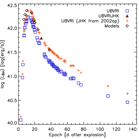
Figure 7: Bolometric light curves for SN 1994I. The squares denote the bolometric light curve obtained from $U\!BV\!R\!I$ observations of SN 1994I without correction for the unobserved $J\!H\!K$ bands. The filled triangle indicates the point for which $J\!H\!K$ is also known. The crosses are the data points obtained by correcting the SN 1994I points for the unobserved $J\!H\!K$ bands by assuming the same contribution as in SN 2002ap. The results of the spectral models are shown as diamonds.

In addition, we derived an upper limit estimate by adding the IR-contribution of SN 2002ap (Yoshii et al., 2003), which is the most similar object for which infrared data have been published. For this addition we assume that the relative contribution of the infrared bands in SN 1994I was the same as for SN 2002ap after the data points of SN 2002ap have been rescaled to the appropriate extinction. The upper limits are shown as crosses in Fig. 7. For SN 1994I additionally one point in each of $J$ and $H$ and two in the $K$ band are available from Rudy et al. (1994). This allows us to compute a single bolometric point for the epoch $t=28\,$d after explosion which is indicated by the filled triangle in Fig. 7. This single point agrees nicely with the upper limit light curve which justifies the choice of the SN 2002ap data to derive the upper limit light curve for SN 1994I. It also shows that the IR contribution to the bolometric flux is not negligible. Generally, for a SN Ic the contribution of the IR-wavelength bands ranges from about $20$ per cent before $B$ maximum, to roughly $40$ per cent near $K$ maximum. In the late phase the IR-bands contribute about $30$ per cent (Yoshii et al., 2003; Patat et al., 2001).

To compute the bolometric light curves, we converted the magnitudes into fluxes using the standard $U\!BV\!R\!I$ Johnson-Cousin system (Buser & Kurucz, 1978; Bessell, 1983). Using $V$ epochs for reference, we then interpolated to these epochs the flux in other bands. The monochromatic fluxes were used as low-resolution spectra and transformed to luminosities adopting a distance modulus of $m-M=29.6\,$mag, an extinction of $E(B\!-\!V)=0.3\,$mag (see §2.1), and the extinction law of Savage & Mathis (1979).

The luminosities used in our spectral models are shown as diamonds in Fig. 7. They are in good overall agreement with the estimate from the observations corrected for the infrared contribution.

4 Light curve models

Figure 8: Synthetic light curve for the modified CO21 ejecta model (solid line) in comparison with the light curve obtained from the original CO21 model (dashed line). The filled circles show the bolometric light curve from the observations (see §3.5).

Fig. 8 shows the synthetic light curve of the ejecta model that we built, as suggested by the nebular-spectrum model, by adding a low-velocity dense core to the density structure of CO21 (solid line), compared with the light curve of the original CO21 (dashed line) and with the bolometric light curve of SN 1994I (circles). We used the one-dimensional supernova light curve synthesis code developed by Iwamoto et al. (2000). The code solves the energy and momentum equations of the radiation plus gas in the co-moving frame and the gray $\gamma$-ray transfer simultaneously; see Mazzali et al. (2002), Deng et al. (2005), and Mazzali (2006) for our approximations on optical line opacities and Eddington factors. The ⁵⁶Ni mass and its distribution were adjusted to optimise the fit. For the relative abundances of other elements, we used the results of our spectral modelling.

Our ejecta model has a total mass of $\sim\!1.2M_{\odot}$, of which $\sim\!0.4M_{\odot}$ is distributed below $5500\,\rm{km\,s}^{-1}$ as required in the nebular spectrum modelling (see § 2.3). For comparison, CO21 has in total $\sim\!0.9M_{\odot}$ with only $\sim\!0.1M_{\odot}$ below $5500\,\rm{km\,s}^{-1}$. The total kinetic energy, $\sim\!1\times 10^{51}\,$erg, is barely changed by the addition of the low-velocity dense core. The best light curve fitting ⁵⁶Ni mass is $\sim\!0.07M_{\odot}$ for both ejecta models, although the distribution of ⁵⁶Ni is different. For CO21, we filled its low-velocity region with as much ⁵⁶Ni as possible without spoiling the fit to the peak to increase the energy deposition rate at late times. This results in $\sim\!0.04$–$0.05M_{\odot}$ of ⁵⁶Ni in the inner $\sim\!0.1M_{\odot}$ ejecta at $v<5500\,\rm{km\,s}^{-1}$. For our ejecta model, which has a core as massive as $\sim\!0.4M_{\odot}$, a ⁵⁶Ni abundance of $\sim\!10$ per cent in that core is enough to reproduce the slow decline of the late-time light curve of SN 1994I, all of which is distributed above $3,000\,\rm{km\,s}^{-1}$ to avoid overestimating the flux around day $\sim\!40$. Both models need a substantial amount of ⁵⁶Ni between $8000$ and $10\,000\,\rm{km\,s}^{-1}$ to reproduce the fast-rising early light curve ($\sim\!0.008M_{\odot}$ for CO21 and $\sim\!0.003M_{\odot}$ for our model). This is consistent with the blue nature of the early spectra, which indicates substantial $\gamma$-ray heating and ${}^{56}\rm{Ni}$ mixing in the outer part of the ejecta (see §3.2).

The light curve of our ejecta model reproduces the observed light curve of SN 1994I well, both in the peak phase (before day $\sim\!30$) and in the tail phase (after day $\sim\!50$). By contrast, the light curve of CO21 declines too fast to follow the observations after day $\sim\!50$ and the discrepancy increases to $\sim\!50$ per cent in flux by day $\sim\!100$. This confirms the results of our nebular spectrum modelling that, compared to CO21, more low-velocity mass is needed to generate the observed line luminosity in the day $159$ spectrum. The low-velocity dense core may suggest that the explosion of SN 1994I was actually aspherical. Spherical explosion models can not produce this dense inner core because they exhibit a cutoff velocity below which material falls back to form the compact object in the center of the explosion. In contrast, models of aspherical explosions generally show a higher density in the inner, low-velocity core because the fall-back region is distorted (e.g., Khokhlov et al., 1999; Maeda et al., 2002, 2003; Mazzali et al., 2004; Tomita et al., 2006). Our model light curve overestimates the flux by $<\!20$ per cent at the transition phase between day $\sim\!30$ and day $\sim\!50$. Further tuning the ⁵⁶Ni distribution and the ejecta density structure in the low-velocity core could solve this discrepancy, which is, however, not significant. On the other hand, this may also be a multi-dimensional effect, the modelling of which is then beyond the scope of this paper.

5 Conclusions

We have re-investigated the properties of the Type Ic supernova SN 1994I because this object is among the best observed “normal” SNe Ic and possibly represents a link between different branches of core-collapse supernovae. The study was based on the density structure of the explosion model CO21 by Iwamoto et al. (1994) although we allowed the composition to deviate from the prediction of this model. Overall the explosion model seems to give a reasonable representation in the outer parts of the ejecta, although the mismatch of the velocities of some features in the early phase may suggest that a density structure with a steeper gradient in the intermediate-velocity range could be more suitable. The nebular-phase models, in contrast, require a significantly larger mass at low velocities than predicted by the model. Our estimate for the ejecta mass inside a radius corresponding to $v=5500\,\rm{km\,s}^{-1}$ is at least $0.4M_{\odot}$. From the photospheric model at $t=24\,$d, which has a photospheric velocity of $5400\,\rm{km\,s}^{-1}$, one can estimate the mass above the outer velocity of the nebular spectrum to be about $0.6M_{\odot}$. This adds up to a value that is larger than the total ejected mass of $0.9M_{\odot}$ of model CO21.

The spectral models also give some indication that the explosion of SN 1994I exhibited some extent of asymmetry or at least inhomogeneity which was able to mix ${}^{56}\rm{Ni}$ out into the oxygen-rich layers. This is also supported by the trend that the abundance of Fe-group elements actually seems to decrease toward the centre of the ejecta. In turn, oxygen-rich material appears to be present at very low velocities as can be seen in the nebular spectrum. In comparison model CO21 does not show much mixing. Recent hydrodynamical simulations (Burrows & Hayes, 1996; Lai & Goldreich, 2000; Scheck et al., 2004) and spectropolarimetric observations (Wang et al., 2001, 2003; Leonard et al., 2002; Leonard et al., 2006) of core-collapse supernova explosions suggest the presence of global asymmetries which could induce large mixing of the ejecta. The overall picture for SN 1994I is that it probably originated from the explosion of a low-mass core that stripped its envelope possibly by binary interaction. The peculiar shape of the early-time spectra, as well as the very fast decline of the light curve show that this object was by no means a “typical” SN Ic. This should be kept in mind when comparisons to other objects are made.

The amount of extinction of SN 1994I by dust is subject to large uncertainties. Our models suggest that the value of $E(B\!-\!V)=0.45\,$mag used by Iwamoto et al. (1994) to model the light curves is probably significantly too large. A value of at most $0.30\,$mag seems more suitable to fit the observed spectra.

Given the constraints on the ejecta mass and reddening from the spectral models, we recalculated the theoretical light curve for the CO21 model with a more massive low-velocity core region. This new model still fits the observed bolometric light curve that we constructed from the spectra well (including a correction for the unobserved infrared bands). To obtain this fit it was necessary to place a substantial amount of ⁵⁶Ni at velocities between $8000$ and $10\,000\,\rm{km\,s}^{-1}$. This supports the corresponding conclusion from the spectral fits. The total amount of ⁵⁶Ni was $\sim\!0.07M_{\odot}$ and did not change compared to the original CO21 model. (The effect of the lower reddening than assumed by Iwamoto et al. (1994) is balanced by a larger distance.)

The nature of the IR-absorption around $10\,300\,$Å cannot be revealed unambiguously on the basis of the methods chosen here. The most likely identification seems to be C i at intermediate velocities with a contribution of He i at high velocities. Neither ion seems to be able to account for the entire absorption without causing unseen features in other parts of the spectrum. C i can also account for other line features which are not reproduced by our models otherwise. A more in depth analysis using a consistent non-LTE treatment of all important processes including non-thermal excitation of He i is needed to provide a more conclusive picture.

References

- Abbott & Lucy (1985) Abbott D. C., Lucy L. B., 1985, ApJ, 288, 679
- Baron et al. (1999) Baron E., Branch D., Hauschildt P. H., Filippenko A. V., Kirshner R. P., 1999, ApJ, 527, 739
- Baron et al. (1996) Baron E., Hauschildt P., Mezzacappa A., 1996, MNRAS, 278, 763
- Bessell (1983) Bessell M. S., 1983, PASP, 95, 480
- Burrows & Hayes (1996) Burrows A., Hayes J., 1996, Physical Review Letters, 76, 352
- Buser & Kurucz (1978) Buser R., Kurucz R. L., 1978, A&A, 70, 555
- Clocchiatti et al. (1996) Clocchiatti A., Wheeler J. C., Brotherton M. S., Cochran A. L., Wills D., Barker E. S., Turatto M., 1996, ApJ, 462, 462
- Deng et al. (2005) Deng J., Tominaga N., Mazzali P. A., Maeda K., Nomoto K., 2005, ApJ, 624, 898
- Feldmeier et al. (1997) Feldmeier J. J., Ciardullo R., Jacoby G. H., 1997, ApJ, 479, 231
- Filippenko et al. (1995) Filippenko A. V. et al. , 1995, ApJ, 450, L11
- Fisher et al. (1999) Fisher A., Branch D., Hatano K., Baron E., 1999, MNRAS, 304, 67
- Harkness et al. (1987) Harkness R. P. et al., 1987, ApJ, 317, 355
- Ho & Filippenko (1995) Ho L. C., Filippenko A. V., 1995, ApJ, 444, 165 [Erratum: 463, 818 (1996).]
- Iwamoto et al. (2000) Iwamoto K. et al., 2000, ApJ, 534, 660
- Iwamoto et al. (1994) Iwamoto K., Nomoto K., Höflich P., Yamaoka H., Kumagai S., Shigeyama T., 1994, ApJ, 437, L115
- Khokhlov et al. (1999) Khokhlov A. M., Höflich P. A., Oran E. S., Wheeler J. C., Wang L., Chtchelkanova A. Y., 1999, ApJ, 524, L107
- Lai & Goldreich (2000) Lai D., Goldreich P., 2000, ApJ, 535, 402
- Leonard et al. (2006) Leonard D. C. et al., 2006, Nat, 440, 505
- Leonard et al. (2002) Leonard D. C. et al., 2002, PASP, 114, 35
- Lucy (1991) Lucy L. B., 1991, ApJ, 383, 308
- Lucy (1999) Lucy L. B., 1999, A&A, 345, 211
- Maeda et al. (2003) Maeda K., Mazzali P. A., Deng J., Nomoto K., Yoshii Y., Tomita H., Kobayashi Y., 2003, ApJ, 593, 931
- Maeda et al. (2002) Maeda K., Nakamura T., Nomoto K., Mazzali P. A., Patat F., Hachisu I., 2002, ApJ, 565, 405
- Mazzali (2006) Mazzali P. A. et al., 2006, ApJ in press (astro-ph/0603516)
- Mazzali (2000) Mazzali P. A., 2000, A&A, 363, 705
- Mazzali et al. (2004) Mazzali P. A., Deng J., Maeda K., Nomoto K., Filippenko A. V., Matheson T., 2004, ApJ, 614, 858
- Mazzali et al. (2002) Mazzali P. A. et al., 2002, ApJ, 572, L61
- Mazzali & Lucy (1993) Mazzali P. A., Lucy L. B., 1993, A&A, 279, 447
- Mazzali & Lucy (1998) Mazzali P. A., Lucy L. B., 1998, MNRAS, 295, 428
- Mazzali et al. (2001) Mazzali P., Nomoto K., Patat F., Maeda K., 2001, ApJ, 559, 1047
- Millard et al. (1999) Millard J. et al., 1999, ApJ, 527, 746
- Nomoto et al. (2003) Nomoto K., Maeda K., Umeda H., Ohkubo T., Deng J., Mazzali P., 2003, in Hucht K. v. d., Herrero A., Esteban C., eds, Proc. IAU Symp. 212, Astron. Soc. Pac., San Francisco, p. 395
- Nomoto & Umeda (2002) Nomoto K., Umeda H., 2002, ASP Conf. Ser. Vol 253, p. 221
- Nomoto et al. (1994) Nomoto K., Yamaoka H., Pols O. R., van den Heuvel E. P. J., Iwamoto K., Kumagai S., Shigeyama T., 1994, Nat, 371, 227
- Patat et al. (2001) Patat F. et al., 2001, ApJ, 555, 900
- Piran (1999) Piran T., 1999, Phys. Rep., 314, 575
- Przybilla (2005) Przybilla N., 2005, A&A, 443, 293
- Richmond et al. (1996) Richmond M. W. et al. 1996, AJ, 111, 327
- Rudy et al. (1994) Rudy R., Dotan Y., Woodward C., Cole J., Hodge T., 1994, IAU Circ., 5991, 3
- Sauer (2005) Sauer D. N., 2005, PhD thesis, Technische Universität München
- Savage & Mathis (1979) Savage B. D., Mathis J. S., 1979, ARA&A, 17, 73
- Scheck et al. (2004) Scheck L., Plewa T., Janka H.-T., Kifonidis K., Müller E., 2004, Phys. Rev. Lett., 92, 11103
- Tominaga et al. (2005) Tominaga N. et al., 2005, ApJ, 633, L97
- Tomita et al. (2006) Tomita H. et al., 2006, ApJ in press (astro-ph/0601465)
- Wang et al. (2003) Wang L., Baade D., Höflich P., Wheeler J. C., 2003, ApJ, 592, 457
- Wang et al. (2001) Wang L., Howell D., Höflich P., Wheeler J., 2001, ApJ, 550, 1030
- Yokoo et al. (1994) Yokoo T., Arimoto J., Matsumoto K., Takahashi A., Sadakane K., 1994, PASJ, 46, L191
- Yoshii et al. (2003) Yoshii Y. et al., 2003, ApJ, 592, 467