Biased Cosmology: Pivots, Parameters, and Figures of Merit

Abstract

In the quest for precision cosmology, one must ensure that the cosmology is accurate as well. We discuss figures of merit for determining from observations whether the dark energy is a cosmological constant or dynamical, with special attention to the best determined equation of state value, at the “pivot” or decorrelation redshift. We show this is not necessarily the best lever on testing consistency with the cosmological constant, and moreover is subject to bias. The standard parametrization of $w(a)=w_{0}+w_{a}(1-a)$ by contrast is quite robust, as tested by extensions to higher order parametrizations and modified gravity. Combination of complementary probes gives strong immunization against inaccurate, but precise, cosmology.

I Introduction

Discovery of the acceleration of the cosmic expansion has precipitated widespread activity and plans to uncover its nature. A significant first question to answer is whether the responsible physics is consistent with a cosmological constant in Einstein’s field equations. Beyond this, we seek to know the dynamics of the dark energy, for example through the value and variation of the equation of state, or pressure to energy density ratio.

In evaluating the leverage of experiments one needs to put forth either a set of benchmark models to distinguish or a model independent parametrization that places a measure or distance in model space. Given the lack of well motivated benchmarks other than the cosmological constant, the second approach is favored in the literature. The ability of an experiment can then be quantified by a figure of merit, ideally rooted in distinctions in the fundamental physics. Recently, the DOE-NASA-NSF Dark Energy Task Force (DETF: detf ) proposed one possible figure of merit, involving the area of the equation of state uncertainty contour.

We examine to what extent this suggestion gets to the heart of the physics, in §II. Moreover, apart from the theoretical precision of a parameter constraint, we must be concerned with the accuracy of the parametrization – the possibility of observational and interpretational bias of the parameters and the cosmology. We consider this from several angles in §III, treating issues of decorrelated parameters, astrophysical evolution and dark energy time variation, and beyond Einstein gravity. In §IV we return to the question of figure of merit and discuss the role of joint confidence contours.

II Figure of merit

How to robustly quantify knowledge of the nature of dark energy is not clear in general. For example, a cosmological constant has a particular value of the equation of state $w=-1$ and lacks any variation, $w^{\prime}\equiv dw/d\ln a=0$. But in the phase plane $w^{\prime}$–$w$ is the optimum measure the area of a likelihood confidence level contour, the volume of the overall N-dimensional (equation of state plus matter density etc. parameters) confidence surface, the largest eigenvalue (shortest dimension of the ellipse defined near the likelihood maximum), etc. (see hutturaip for an early discussion of some of these)?

This difficulty persists even if we restrict to the narrow question of whether the dark energy is a cosmological constant $\Lambda$ or not. If we strive to optimize the determination of the value $w$ at some redshift, obtaining a so-called sweet spot or pivot value $w_{p}$, we can be misled. Even if we determine the value $w_{p}$ is -1 the variation $w^{\prime}$ is still important since models distinct from $\Lambda$ exist where $w_{p}=-1$, $w^{\prime}\neq 0$. Indeed in §III.5 we will show that biased parametrization can lead to exactly this situation.

In a completely blank phase space, minimizing the area of the equation of state contour, as proposed by the DETF in the gaussian approximation, is a good strategy. However, we are not completely blind to the structure of the physics; Fig. 1 shows distinct, physically motivated regions identified by caldlin due to the overall dynamics of scalar fields and further generalizations including modified gravity paths . Thawing models evolve away from the cosmological constant state and possess $1+w<w^{\prime}<3(1+w)$, while freezing models move toward the cosmological constant and today lie in $0.5w(1+w)\gtrsim w^{\prime}>3w(1+w)$. (In the figure we translate to $w_{a}=-2w^{\prime}|_{z=1}$ to fit the standard parametrization used in the rest of the paper.) This physical structure suggests specific strategies for optimizing our knowledge of dark energy.

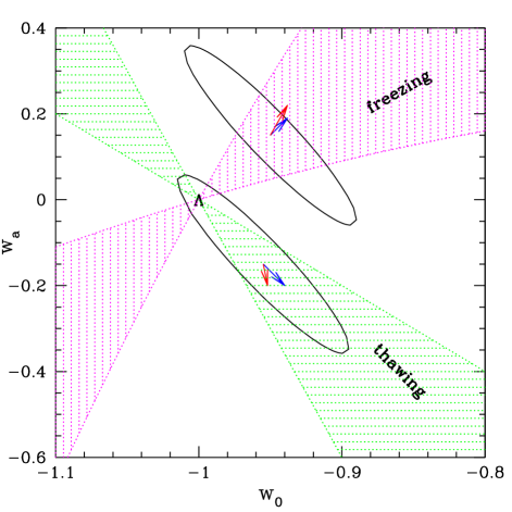
Figure 1: By using the physical structure of the dark energy phase plane, we find optimal quantities for figures of merit for different regions. The shaded areas show the freezing and thawing classes caldlin ; they intersect at the cosmological constant $\Lambda$. Confidence contours from next generation cosmological observations are shown for two dark energy models, one in each class, pointing up very different criteria for distinguishing them from $\Lambda$ (dark, blue arrows) or from the other class (light, red arrows).

While there are benefits to uniform shrinking of error contours (which translates to minimizing $\sigma(w_{p})\times\sigma(w_{a})$ in the gaussian approximation), the phase space structure shows other approaches can be more valuable. For a model in the freezing region, we see that more tightly constraining the narrow dimension of the contour, corresponding to the largest eigenvalue, is near optimal to distinguish the data from the cosmological constant – and to separate it from the other physical class of the thawing behavior.

However, for a model in the thawing region, limiting the long dimension of the contour (the smallest eigenvalue), is the key discriminant from $\Lambda$. Indeed, experiments that are only sensitive to an averaged equation of state (such as most planned ground based experiments, due to limited redshift baseline) have a degeneracy direction squarely through the thawing region, making it virtually impossible for these to distinguish that half of physics classes from the cosmological constant. Beyond $\Lambda$, to maximally separate data pointing to the thawing region from freezing models one would seek to constrain the contour along nearly the vertical direction.

The uncertainty $\sigma(w_{p})$ in the pivot value $w_{p}$ (see the next section for exactly what is a pivot) corresponds not to the short dimension of the contour, but the width of the contour at fixed $w^{\prime}$ (or $w_{a}$), i.e. $w^{\prime}$ held to its fiducial value and not treated as a free parameter. This gives a horizontal cut slanting across the contour, not along the short axis (unless the equation of state variables are uncorrelated; see §IV for illustration of this and further discussion). Minimizing the horizontal width of the contour only gives the optimal science in the special case when the data lie horizontally offset from the cosmological constant – i.e. in the “no model’s land” between the freezing and thawing regions, where the scalar field potential is fine tuned to balance the kinetic energy just so to give a constant value $w$. Furthermore, horizontal squeezing of the confidence contour is never optimal for distinguishing the freezing and thawing classes.

Table 1 summarizes the optimal characteristics to constrain – “figures of merit” – for greatest science return on the dark energy equation of state. Clearly no one figure of merit is optimal in all circumstances. However, we do not know how to weight the likelihood that the true model will lie in a particular region of phase space, so it is difficult to look for even a “best average” figure of merit, that gives the greatest good for the greatest numbers, or greatest insight for the greatest likelihood of cases. We discuss this further in §IV.

Table 1: Figures of merit vary for different circumstances. Case denotes the region where the true universe lies (blank meaning all points in phase space are equivalent). Goal denotes the science objective, e.g. distinction from $\Lambda$ or between thawing and freezing classes.

Case	Goal	Figure of Merit
Blank	Anything	Area
Thawing	$\Lambda$	Long axis
Thawing	vs. Freezing	$\sim w_{a}$
Freezing	$\Lambda$	Short axis
Freezing	vs. Thawing	$\sim$ Short axis
Defect	$\Lambda$	$w_{p}$

What would be beneficial is the power to significantly alter the orientation of the contours at a given fiducial point in the phase space. If we could rotate the contour around a thawing model 90 degrees then these would be more easily distinguishable from a cosmological constant (whereas freezing models would be less so). This is completely different from constraining $w_{p}$, i.e. minimizing $\sigma(w_{p})$, however. The orientation, or main degeneracy direction, is related to the pivot redshift $z_{p}$ itself, and is a property of the cosmological probe, or combination of probes, used. Our desired 90 degree rotation corresponds to a negative $z_{p}$. Practical probes all tend to have nearly the same degeneracy direction (see, e.g., coorayhut ) and combining probes averages the direction, so it is very difficult to rotate the contours even tens of degrees. (Note that strong lensing does provide a way to obtain $z_{p}<0$ linsl , but systematics distort the contour so as to prevent significantly useful rotation.)

To understand the heart of dark energy physics we need high precision to constrain the dynamics $w^{\prime}$–$w$; we have seen that a figure of merit for that precision is nontrivial. But we also must make sure that the cosmology fitting and its interpretation are accurate, that there is negligible bias. From Fig. 1 we see that a shift in the best fit parameters could easily move a thawing model, say, to a result appearing as the cosmological constant or a freezing model. Moreover, we must test the parametrization of the phase plane itself, to ensure that with a few parameters we robustly capture the key physics. The next section studies these two issues, of bias in the observations and in the interpretation.

III Bias

For model independent treatment of the equation of state (EOS) phase space $w^{\prime}$–$w$, the standard parametrization contains two parameters, describing the value and variation of the EOS:

$$w(a)=w_{0}+w_{a}(1-a).$$ (1)

This is well known to be accurate in describing a wide variety of physical models linprl ; paths . Moreover, linhut05 demonstrated that even next generation observations would be generically capable of tightly constraining only two parameters. However, they pointed out that extended or higher order parametrizations could be useful in assuring the resistance to bias of the fitted cosmological parameters.

Another possibility for dark energy parametrization is the closely related form employing decorrelated variables,

$$w(a)=w_{p}+w_{a}(a_{p}-a).$$ (2)

Here the pivot redshift astier ; huttur ; welal $z_{p}=a_{p}^{-1}-1$ is chosen such that $w_{p}\equiv w(z_{p})$ and $w_{a}$ are uncorrelated. Known drawbacks of this parametrization include the dependence of $z_{p}$ and hence $w_{p}$ on the method of probing the cosmology, the specific experiment design, the fiducial model, and the priors employed. This dependence causes a lack of independent physical meaning of $w_{p}$, i.e. $w_{p}$ from one specific experiment for learning about the universe cannot be directly and generally compared to the $w_{p}$ value from another. The plus side is that $w_{p}$ can be more precisely determined than $w_{0}$, and indeed is the most precisely determined single value of $w(z)$.

The question we take up here is whether the $w_{p}$–$w_{a}$ parametrization is also more accurately determined than $w_{0}$–$w_{a}$. We examine their robustness against theoretical and observational biases that lead to a shift in the fitted parameters.

Parameter biases $\delta p_{i}$ induced from offsets $\Delta O_{k}$ in the observable quantities are calculated using the Fisher formalism, where maximizing the likelihood leads to

$$\mathbf{\delta p}=A\,\mathbf{\Delta O}=\left(U^{T}C^{-1}U\right)^{-1}U^{T}C^{-1}\mathbf{\Delta O},$$ (3)

where $\mathbf{O}$ is the vector of expected observations, $C$ is the covariance matrix of observational errors, and $U=\partial O/\partial\mathbf{p}$. Put more simply, when the covariance matrix is diagonal,

$$\delta p_{i}=(F_{\rm tot}^{-1})_{ij}\sum_{k}\frac{\partial O_{k}}{\partial p_{j}}\frac{1}{\sigma_{k}^{2}}\,\Delta O_{k},$$ (4)

and $O_{k}$ is the $k$th observable (e.g. supernova magnitude at some redshift bin), $\Delta O_{k}$ is the observational quantity offset (due to either theory error or systematic measurement error), and $F_{\rm tot}$ is the Fisher matrix from all observables. We consider the cosmological probe of the distance-redshift relation for $z=0-1.7$, as from a future survey of Type Ia supernovae by the Supernova/Acceleration Probe (SNAP snap , which of course includes systematics), together with future measurement of the distance to the cosmic microwave background (CMB) last scattering surface, as from Planck planck .

III.1 Extended time variation

Disallowing any time variation in the dark energy EOS, i.e. holding the value $w$ constant for all redshifts or fitting only an averaged value, not only obscures the physics but even biases the constant or averaged value (e.g. maor ). The $w_{a}$ parametrization removes that difficulty by allowing for variation, $w_{a}=-dw/da$. We should ensure, however, that there is not a continued hierarchy of bias, i.e. that neglecting a second derivative term does not bias the measured variation $w_{a}$.

To some extent, this robustness is already taken care of by the physical foundation of the $w_{a}$ parametrization – that it was designed specifically to model accurately the exact effect of a range of dark energy models (unlike the vast majority of alternate parametrizations). Nevertheless, it is worth explicitly demonstrating the robustness.

To do this, we adopt a parametrization with an explicit second derivative $d^{2}w/da^{2}\neq 0$. We choose Model 3.1 from linhut05 ,

$$w(a)=w_{0}+w_{a}(1-a^{b}),$$ (5)

again because of its physical foundation as discussed in linhut05 . Now $d^{2}w/da^{2}=-b(b-1)w_{a}a^{b-2}$. The phase space behavior is given by $w^{\prime}=b(w-w_{\infty})$, where $w_{\infty}$ is the high redshift value of $w$. By considering cases corresponding to both freezing and thawing models (evolution toward and away from cosmological constant behavior, respectively), we can investigate the stability of the first derivative only ($w_{a}$) parametrization.

First, consider a freezing model with $w_{0}=-0.9$, $w_{a}=0.2$. As we change $b$ from its canonical value of unity, but attempt to fit the cosmology within the standard parametrization, we will unavoidably bias the values of the cosmological parameters. Figure 2 shows the fractional bias $\delta p/\sigma(p)$, i.e. how many standard deviations the parameter $p$ is offset, for joint estimation of $\{\Omega_{m},w_{0},w_{a}\}$ or alternately $\{\Omega_{m},w_{p},w_{a}\}$ (plus any nuisance parameters). That is, we compare the robustness of parametrization (2) vs. (1). While $w_{0}$ is essentially unbiased, $w_{p}$ can suffer bias at a significant fraction of the $1\sigma$ statistical uncertainty ($w_{a}$ and $\Omega_{m}$ are negligibly affected). Note that the dark energy model considered here lies within the freezing region $w(1+w)\gtrsim w^{\prime}>3w(1+w)$ for $b=0.45$–1.35.

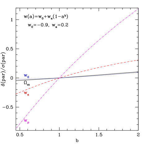
Figure 2: Dark energy with more complex time variation than the standard two parameter model, but interpreted in terms of $w_{0}$, $w_{a}$, will bias the parameter estimation. Here we consider observational constraints from next generation supernova and CMB measurements on a three parameter model in the freezing class. The $w_{0}$ and $w_{a}$ parameters are quite robust, nearly unbiased, but the sweet spot, or pivot, value $w_{p}$ can be appreciably misestimated.

Next we consider the thawing class of models. As mentioned in linhut05 , when the high redshift value of the EOS $w_{\infty}=-1$, i.e. starting from a frozen, cosmological constant like state, then the parametrization (5) describes a line of slope $b$ in the phase plane: $w^{\prime}=b(1+w)$, an excellent approximation to a wide variety of physics models such as power law potentials and pseudo-Nambu Goldstone boson models. The thawing region $1+w<w^{\prime}<3(1+w)$ is obtained for $b=1$–3.

Figure 3 illustrates that again the fractional bias is well under control for the $w_{0}$–$w_{a}$ parametrization, but that $w_{p}$ is subject to large biases. At the upper end of the thawing region, where $b=3$, $w_{p}$ can be shifted by 1.7$\sigma$, an unacceptable bias to the cosmology. This opens up the prospect of both false positives and false negatives, where we either mistakenly think we have confirmed the cosmological constant to high precision or incorrectly claim evidence for deviation from the cosmological constant despite $\Lambda$ being true. In contrast, $w_{0}$ is misestimated by less than 0.3$\sigma$ (and $w_{a}$ and $\Omega_{m}$ are also cleanly recovered).

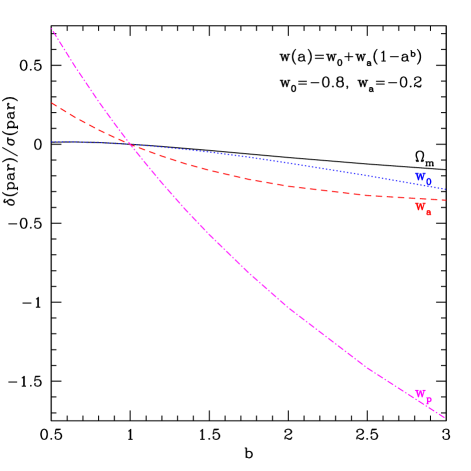
Figure 3: As Fig. 2, but for a model evolving away from a high redshift cosmological constant like state, i.e. thawing.

So the $w_{0}$–$w_{a}$ parametrization is an excellent, fair description of the cosmological model even when the dark energy has extended time variation, in both the freezing and thawing classes of physics. These classes describe many standard, physically motivated scenarios (see caldlin ; paths for a wide variety of both scalar field and modified gravity models). However one can certainly postulate other behaviors with more extreme time variation. We test the standard parametrization to the breaking point in the next section.

III.2 Rapid transition

Rapid transitions in dark energy behavior cannot be well fit by the simple two parameter model. In this case, one might require four parameters – asymptotic past and future values, time of transition, and rapidity of transition – as discussed in linhut05 . That article put forward a solution in Model 4.0, the e-fold model,

$$w(a)=w_{f}+\frac{\Delta w}{1+(a/a_{t})^{1/\tau}},$$ (6)

where $w_{f}$ ($w_{\infty}$) is the asymptotic future (past) value, $\Delta w=w_{\infty}-w_{f}$, $a_{t}$ the transition scale factor, and $\tau$ the rapidity (note that in paths , $\tau$ was the reciprocal of the rapidity).

As the transition becomes more rapid, we expect the two parameter model to have greater difficulty fitting this behavior, and hence greater bias in the parameter estimation. Within the e-fold parametrization, $\tau$ gives the characteristic e-folding scale of the transition, with $\tau=1$ corresponding to a Hubble time at the transition redshift. This provides a natural scale, and one might expect that inertia in the field evolution could lengthen the transition to $\tau\gtrsim 1$.

Figure 4 shows the bias effects of a cosmology with an e-fold parametrization behavior but interpreted in terms of $w_{0}$–$w_{a}$ or $w_{p}$–$w_{a}$. As expected, the two parameter models are good fits for slow transitions, but not for rapid transitions. The parameter behavior also depends on the magnitude of the transition $\Delta w$; here we fix $w_{f}=-1$ and use $w_{\infty}=\Delta w-1$ as the independent variable, also taking $w_{0}=-0.9$ as fiducial. Parametrizing in terms of $w_{p}$ begins to be appreciably biased for $\tau\lesssim 2$, while $w_{0}$ stays a fair estimator to $\tau\gtrsim 0.5$. The bias in $w_{a}$ tends to be greater than that in $w_{0}$ (and is slightly greater than in $\Omega_{m}$), but is still acceptable for $\tau\gtrsim 0.7$.

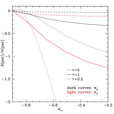
Figure 4: As Fig. 2, but for the e-fold model, as a function of $w_{\infty}=w(z\gg 1)$, with $w_{0}=-0.9$. When the equation of state evolution is rapid (small $\tau$), then estimates of the equation of state from the observations are increasingly biased. The pivot value $w_{p}$ (light, red curves) is most distorted, while $w_{a}$ (dark, black curves) is fairly robust (and $w_{0}$, not shown, is more so), except for very sharp transitions.

As the limit of an extreme transition we can consider a step function in the EOS at some redshift $z_{c}$. Even for small steps this can produce a large bias in $w_{p}$, and again the fractional bias in $w_{0}$ is less. Note that simpsonbridle found that for an increasing EOS one could in fact obtain a bias giving a counterintuitive negative $w_{a}$. While such eigenmode decomposition of the EOS is an elegant approach, the Fisher bias formalism equivalently gives the weight or “redshift sensitivity” functions for parameter fitting (and can handle more general situations, as seen in following sections). The seemingly paradoxical bias result is explained by the degeneracies among the parameter set: while $w_{a}$ may be biased down, $w_{0}$ or $\Omega_{m}$ would be biased up to compensate.

The possibility of individual parameters flopping around through degeneracies, even to the opposite sign, cautions against interpretation relying on a single parameter (as was done with constant $w$ in the early days). Analogously, it is important not to rely on a single probe. For the exact case considered by simpsonbridle , the opposite direction paradox goes away if one considers both supernovae and CMB distance measurements, as the degeneracy is then restricted.

III.3 Evolving observable

While we have so far considered the bias due to theory, in terms of parametrization, we can apply the same formalism to systematic offsets in the measurements. For supernovae, treatments include the possibility of evolving luminosity (e.g. astier ; welal ; klmm ) and gravitational lensing amplification bias holzlinder . Effects due to heterogeneous data sets were discussed in linmiq and systematics in dust extinction properties in lintaup . The propagation of systematic errors through to cosmological parameter biases is unfortunately less common for other cosmological probes (but see huttak for a nice treatment within weak gravitational lensing, and mohr for one instance for cluster masses).

Here we combine the two issues by examining how a measurement systematic interacts with the theory parametrization. We take a hypothetical offset in supernova luminosity in terms of the absolute magnitude parameter $\Delta M(z)\equiv M(z)-M(0)=\alpha(1-a)$. This could perhaps arise from population drift in supernova environments or progenitor systems (without attempting rigorous justification, we note that the offset should be bounded as the redshift gets large, especially as the cosmic time intervals grow shorter and the diversity of environments decreases). We find that the resulting parameter biases can be written as

$$\frac{\delta p}{\sigma(p)}=X(p)\,\frac{\Delta M(z=1.7)}{0.02},$$ (7)

with $X(\Omega_{m},w_{0},w_{a},w_{p})=-0.55$, -0.14, -0.08, -0.50. So as before, $w_{p}$ is substantially more biased in units of standard deviation than $w_{0}$. While $w_{a}$ is very fairly estimated, now $\Omega_{m}$ is affected. Note, however, that at the level of $\Delta M=0.02$ between $z=0$ and 1.7 the cosmology fit is not strongly affected; e.g. the quadrature sum of dispersion and bias is increased by less than 14% relative to no magnitude evolution.

If instead we treat possible evolution as an extra fit parameter $\alpha$, this removes the bias, replacing it with an increased dispersion. With a gaussian prior of 0.04 mag on $\Delta M(z=1.7)$, the parameter estimation uncertainty on $w_{0}$ increases by 4%, but on $w_{p}$ increases by 41%, relative to the no evolution case (the dispersion in $w_{a}$ increases by 1% and in $\Omega_{m}$ by 49%). Of course, exchanging a systematic bias for a new fit parameter and increased dispersion only works if one knows the functional form of the systematic – that is the whole basis of “self-calibration”.

III.4 Modified gravity

The expansion history is specified by the equation of state ratio $w(a)$, but the history of growth of structure in the universe depends on both the expansion history and the theory of gravity. If gravity is modified from general relativity, then the observables involving growth will be offset from the general relativity predictions. This in turn will cause a bias in cosmological parameters interpreted within the framework of Einstein gravity.

Effects from modification of gravity can be quite complex, and there is no general treatment even in the linear regime of structure formation. One approach is the growth index parametrization of groexp ; this has been shown highly accurate in the linear growth factor for taking into account expansion history effects, and modified gravity in the DGP dgp braneworld model. Another interesting approach, not yet fully developed, is phenomenological modification of the Poisson equation giving the source term of the growth equation; this will give a scale dependent growth factor stabenaujain .

In the growth index formalism, the linear growth factor of matter density perturbations $g(a)=(\delta\rho/\rho)/a$ is given by

$$g(a)=e^{\int_{0}^{a}da/a\,[\Omega_{m}(a)^{\gamma}-1]},$$ (8)

where $\gamma$ is the growth index. For a matter plus cosmological constant universe, $\gamma=0.55$, and the formula is accurate to better than 0.05%. Modification of gravity will shift $\gamma$; for example the DGP growth factor is well fit (to 0.2%) by $\gamma=0.68$.

To propagate the effects of modified gravity on growth through to cosmological parameter bias we offset $\gamma$ from the general relativity value. We then add future measurements giving the linear growth factor at $z=0$, 0.4,…2.8 to 2% precision to the previously considered supernova and CMB distance observations. As shown in Fig. 5, again $w_{p}$ is strongly biased, while $w_{0}$ is scarcely affected. Deviations in $w_{a}$ are minor, and in $\Omega_{m}$ are appreciable but not severe for $|\Delta\gamma|<0.05$.

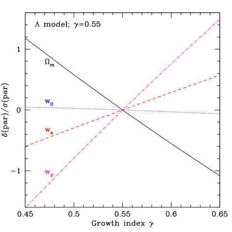
Figure 5: Modification of gravity, if interpreted in an Einstein gravity context, will bias the cosmological parameter estimation. Here we consider observational constraints from next generation linear growth factor measurements to 2% over $z=0-2.8$, plus supernova and CMB measurements; the modified gravity is parametrized through the growth index $\gamma$ groexp , with $\gamma=0.55$ in general relativity. The $w_{0}$ and $w_{a}$ parameters are reasonably robust, but the sweet spot, or pivot, value $w_{p}$ (and to a less extent the matter density $\Omega_{m}$) can be appreciably biased.

III.5 Density parametrization and crossover bias

We have emphasized that parametrizations should be robust, i.e. unbiased. This means that they must be crafted specifically for the questions we want answered. If a parameter $P$ is robust, i.e. its fit value equals the expectation value, then $P^{2}$ or more generally some nonlinear function $f(P)$ is not unbiased. Thus if we want to learn about the dynamics $w^{\prime}$–$w$ of dark energy, we should parametrize the equation of state directly.

Using other quantities such as dark energy density $\rho$ or Hubble parameter $H$ as a basis for parametrization is known to be improper and dangerous, when the aim is the dark energy equation of state. For example, jonsson clearly demonstrated the instability and bias in $w(a)$ from adopting a functional form for $\rho(z)$ or $H(z)$, and recon showed that binned values $\rho(z_{i})$ had similar pathology (although recon pointed out that binned values in $a$ or $\ln(1+z)$ are subject only to the usual, still worrying, numerical instabilities).

Instabilities often lead to crossover behavior, where spurious evolution, e.g. from $w<-1$ to $w>-1$ occurs. jonsson showed instances where this necessarily happened close to the minimum variance location – i.e. $w_{p}\approx-1$ was forced. Perhaps the earliest crossover models were given by lingrav (the crossing of $w=-1$ is now sometimes called the “phantom divide” hu04 ) and have some interesting properties relevant to parameter bias. When implemented by two scalar fields,

$$w(z)=w_{1}\frac{\delta H_{1}^{2}}{\delta H_{1}^{2}+\delta H_{2}^{2}}+w_{2}\frac{\delta H_{2}^{2}}{\delta H_{1}^{2}+\delta H_{2}^{2}},$$ (9)

where $\delta H_{i}^{2}$ is the contribution of component $i$ to the Hubble expansion equation, the dependence of $w(z)$ on the parameters $w_{i}$ and $w_{j}$ becomes nonlinear, and errors in their determination lead to the error in the reconstructed $w(z)$ running away as $\ln(1+z)$. This can even lead to false crossover behavior despite both fields having $w>-1$, say. Because observations tell us that the averaged value of $w$ is not too different from -1, this means that any crossover must have happened at reasonably low redshift – i.e. the crossover redshift must be fairly close to the pivot redshift, forcing $w_{p}\approx-1$.

(Note also that observational systematics as in §III.3 can bias $w_{0}$ one way and $w_{a}$ the other way, possibly causing a crossover. A simple model where the local Hubble flow supernovae, measured with different instrumentation than higher redshift supernovae, are offset in magnitude from the others can fulfill this condition. Hence, great care must taken with calibration, and a single experiment should cover as much of the full redshift range as possible.)

IV Confidence contours

The considerations and calculations in this paper point out that the most precisely determined value of $w(z)$ – i.e. $w_{p}$ – can also be the most sensitive to bias and misinterpretation of the nature of the dark energy from improper parametrization or observational systematics.

The presence of bias does not herald failure for understanding dark energy but rather advocates for caution in interpretation and for complete description of the parameter estimation. As shown, robust parametrization can obviate many of the problems, and, as in §III.3, one can cure bias by judiciously chosen additional fit parameters.

One should also distinguish between the absolute parameter bias $\delta p$ and the fractional bias $\delta p/\sigma(p)$; in many cases the fractional bias on $w_{p}$ is larger than on $w_{0}$ because $w_{p}$ is more precisely determined. Still, if $w_{p}$ is used to advertise precision, the fractional bias tells to what extent this is an accurate result. Statisticians often combine the precision, or dispersion $\sigma(p)$, with the bias $\delta p$ to form the “risk” on a parameter,

$$r(p)=\sqrt{\sigma^{2}(p)+\delta p^{2}}=\sigma(p)\,\left(1+[\delta p/\sigma(p)]^{2}\right)^{1/2}.$$ (10)

We see that the fractional bias then gives the increase from the statistical dispersion to the parameter risk. For many of the cases discussed in this paper, despite a higher fractional bias than $w_{0}$, $w_{p}$ still has a lower overall risk.

Risk, however, is a matter of personal comfort not rigorous mathematics, in cosmology as in the stock market. Rather than having statistical precision and bias contribute equally, as in Eq. (10), we might be willing to pay a premium to have great confidence in our understanding of fundamental physics, and weight robustness and low bias more strongly than mere statistical precision. If we want to avoid false conclusions about, say, whether something other than the cosmological constant pervades our universe, we should seek experiments and parametrizations that stringently control bias.

In any case, quoting a single parameter’s statistical precision, bias, or risk withholds important information due to correlations between parameters. The likelihood surface for the set of parameters (usually shown as a two parameter confidence contour, marginalized or minimized over the other parameters) retains and illustrates information on dispersion, bias, and degeneracies.

Figure 6 illustrates the confidence contours for various fiducial models in the case of §III.3 where an observational offset in supernova magnitudes as a function of redshift biases the cosmological parameters. To show the bias clearly, we adopt $\Delta M(z=1.7)$ such that $w_{p}$ is biased by $1\sigma$ in each case, and plot the $1\sigma$ projected confidence contour (39% confidence level), so the biases can be read off directly from projection to the axes. We simultaneously show the $w_{0}$–$w_{a}$ and $w_{p}$–$w_{a}$ planes: the solid, black contours are for the $w_{0}$ cases, and the three legged symbol shows the best fit, while the dashed, red contours are for the $w_{p}$ cases and the x shows the best fit. Each true cosmological model is indicated by the blue stars, one for $w_{0}$, one for $w_{p}$. The measurement offset biases the parameter estimation such that $w_{0}$ is much less biased in the fractional sense (and in this case in the absolute sense as well). However, the true model lies at an equal confidence level in either parametrization.

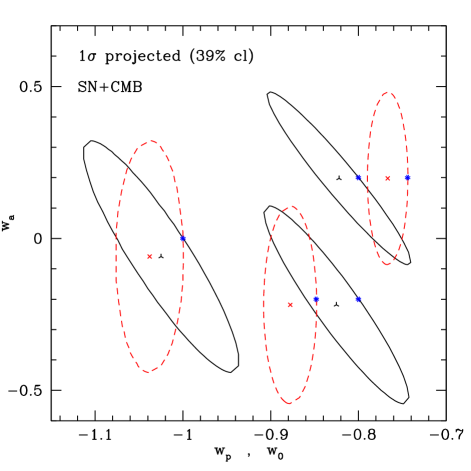
Figure 6: Likelihood contours provide a fairer depiction of bias than one dimensional parameter uncertainties. Various fiducial models (with their $w_{0}$ and $w_{p}$ values indicated simultaneously by blue stars) are biased to new values of $w_{0}$, $w_{p}$ by differing amounts (respectively shown by black, three legs and red x’s), but remain at the same confidence level. Contours in $w_{p}$–$w_{a}$ space are always vertical, and their degeneracy axis intersects the degeneracy axis of the tilted $w_{0}$–$w_{a}$ contours at $w_{a}=0$ (and the contour widths for $w_{a}=0$ are equal in either parametrization).

In terms of the individual parameters, then, $w_{0}$ tends to be more robust than $w_{p}$ for the fractional bias, and one should be wary of treating quotes of statistical precision of $w_{p}$ as robust. Better is to show the joint likelihood surface or confidence contour, which does provide an even handed assessment of bias. We saw in §II that the physical incisiveness of the contours depends on both the parametrization and location in phase space. The vertically oriented contours of $w_{p}$–$w_{a}$ are optimal only in the “dead zone” between the physically motivated freezing and thawing behaviors (see caldlin ; paths ). Similarly, the area of the contour, equal in either plane hutturaip and conveniently written in the gaussian approximation as $\sigma(w_{p})\times\sigma(w_{a})$, is the optimal figure of merit only in the Snarkian sense.

V Conclusion

Understanding the new physics lying behind the acceleration of the cosmic expansion requires precision in the measurements, accuracy in the measurements, and robustness in the interpretation of the data. We have tested the concept of the two parameter dark energy equation of state phase plane and demonstrated further that the standard $w_{0}$–$w_{a}$ parametrization provides a robust framework for interpreting dark energy, considering systematic errors in the observations, more complex dark energy models, and gravity beyond general relativity. The pivot, or decorrelation, value of the equation of state, $w_{p}$, is more subject to bias from such effects.

Seeing the true nature of dark energy, not a subjective, biased interpretation, is an exciting challenge. Robust parametrization, yielding a fair, unbiased answer is one step, and points the way to another: complementarity of probes plays a crucial role. We saw at the end of §III.2 that a sufficiently rapid transition in the dark energy behavior could lead not only to a bias, but one that in a single parameter acts opposite to the direction of the transition, spoofing the nature of the dark energy. Combining more than one cosmological probe immunizes against this, by reducing the degeneracies that allow such an extreme distortion – as well as guarding against systematic errors (or beyond Einstein gravity) that can also bias results.

We found that one must be wary of uncertainties quoted on individual parameters, such as $w_{p}$ that anyway lacks a standalone physical basis, varying based on the probe, survey, priors, and fiducial model. The likelihood, or confidence contours in the equation of state plane, is a fairer depiction of the consistency of models with data. A single optimal figure of merit cannot be defined, however, for the dark energy phase space, but is informed by the physical structure of the dynamics, e.g. thawing and freezing regions. The use of the area of contour ellipses as proposed by the Dark Energy Task Force is ok, though limited, but one should not overinterpret the role of $w_{p}$ for calculating the area as promoting $w_{p}$ to a favored parameter, due to its flaws.

In fact, we seem led to either custom figures of merit following the physics in the robust $w_{0}$–$w_{a}$ parametrization or to taking another look at defining a series of benchmark models. Either way, the firm foundation of the dynamics $w^{\prime}$–$w$ and the standard parametrization provides realistic hope for learning the true nature of the cosmic acceleration.

References

-
(1)
http://www.nsf.gov/mps/ast/detf.jsp ;
https://www.darkenergysurvey.org/the-project/news/ AAAC_presentation - (2) D. Huterer & M.S. Turner, AIP Conf. Proc. 599, 140 (2001) [astro-ph/0006419]
- (3) R.R. Caldwell & E.V. Linder, Phys. Rev. Lett. 95, 141301 (2005) [astro-ph/0505494]
- (4) E.V. Linder, Phys. Rev. D 73, 063010 (2006) [astro-ph/0601052]
- (5) D.N. Spergel et al., astro-ph/0603449
- (6) A. Cooray, D. Huterer, D. Baumann, Phys. Rev. D 69, 027301 (2004) [astro-ph/0304268]
- (7) E.V. Linder, Phys. Rev. D 70, 043534 (2004) [astro-ph/0401433]
- (8) E.V. Linder, Phys. Rev. Lett. 90, 091301 (2003) [astro-ph/0208512] ; E.V. Linder, in Identification of Dark Matter (IDM2002), eds. N.J.C. Spooner & V. Kudryavtsev (World Scientific: 2003) [astro-ph/0210217]
- (9) E.V. Linder & D. Huterer, Phys. Rev. D 72, 043509 (2005) [astro-ph/0505330]
- (10) P. Astier, Phys. Lett. B 500, 8 (2001) [astro-ph/0008306]
- (11) D. Huterer & M.S. Turner, Phys. Rev. D 64, 123527 (2001) [astro-ph/0012510]
- (12) J. Weller & A. Albrecht, Phys. Rev. D 65, 103512 (2002) [astro-ph/0106079]
-
(13)
http://snap.lbl.gov ;
G. Aldering et al., astro-ph/0405232 - (14) http://planck.esa.int
- (15) I. Maor, R. Brustein, J. McMahon, P.J. Steinhardt, Phys. Rev. D 65, 123003 (2002) [astro-ph/0112526]
- (16) F. Simpson & S. Bridle, Phys. Rev. D 73, 083001 (2006) [astro-ph/0602213]
- (17) A.G. Kim, E.V. Linder, R. Miquel, N. Mostek, MNRAS 347, 909 (2004) [astro-ph/0304509]
- (18) D.E. Holz & E.V. Linder, ApJ 631, 678 (2005) [astro-ph/0412173]
- (19) E.V. Linder & R. Miquel, Phys. Rev. D 70, 123516 (2004) [astro-ph/0409411]
- (20) E.V. Linder, plenary talk at TAUP2005 – http://supernova.lbl.gov/~evlinder/taup.ppt
- (21) D. Huterer & M. Takada, Astropart. Phys. 23, 369 (2005) [astro-ph/0412142]
- (22) J.J. Mohr, B. O’Shea, A.E. Evrard, J. Bialek, Z. Haiman, Nucl. Phys. B Proc. Suppl. 124, 63 (2003) [astro-ph/0208102]
- (23) E.V. Linder, Phys. Rev. D 72, 043529 (2005) [astro-ph/0507263]
- (24) G. Dvali, G. Gabadadze, M. Porrati, Phys. Lett. B 485, 208 (2000) [hep-th/0005016]; C. Deffayet, G. Dvali, G. Gabadadze, Phys. Rev. D 65, 044023 (2002) [astro-ph/0105068]
- (25) H.F. Stabenau & B. Jain, astro-ph/0604038
- (26) J. Jonsson, A. Goobar, R. Amanullah, L. Bergstrom, JCAP 09, 007 (2004) [astro-ph/0404468]
- (27) E.V. Linder, Phys. Rev. D 70, 061302 (2004) [astro-ph/0406189]
- (28) E.V. Linder, Phys. Rev. D 70, 023511 (2004) [astro-ph/0402503]
- (29) W. Hu, Phys. Rev. D 71, 047301 (2005) [astro-ph/0410680]
- (30) H. Cramér, “Mathematical methods of statistics”, §32.3 (Princeton U. Press: 1946); M. Kendall & A. Stuart, “Advanced Theory of Statistics”, 4th ed., §17 (Oxford U. Press: 1979)