Unveiling Hidden Patterns in CMB Anisotropy Maps

Abstract

Bianchi VII_h models have been recently proposed to explain potential anomalies in the CMB anisotropy as observed by WMAP. We investigate the violation of statistical isotropy due to an embedded Bianchi VII_h templates in the CMB anisotropy maps to determine whether the existence of a hidden Bianchi template in the WMAP data is consistent with the previous null detection of the bipolar power spectrum in the WMAP first year maps. We argue that although correcting the WMAP maps for the Bianchi template may explain some features in the WMAP data it may cause other anomalies such as preferred directions leading to detectable levels of violation of statistical isotropy in the Bianchi corrected maps. We compute the bipolar power spectrum for the low density Bianchi VII_h models embedded in the background CMB anisotropy maps with the power spectrum that have been shown in recent literature to best fit the first year WMAP data. By examining statistical isotropy of these maps, we put a limit of $(\frac{\sigma}{H})_{0}\leq 2.77\times 10^{-10}(99\%CL)$ on the shear parameter in Bianchi VII_h models.

I Introduction

Friedmann-Robertson-Walker (FRW) models are the simplest models of the expanding Universe which are spatially homogeneous and isotropic. When proposed, the principal justification for studying these models was their mathematical simplicity and tractability rather than observational evidence. However, we now have observational evidence from the isotropy of CMB and large scale structure that the universe on large scales must be very close to that of a FRW model. However, there still remains some freedom to choose homogeneous models that are initially anisotropic but become more isotropic as the time goes on, and asymptotically tend to a FRW model. Bianchi models provide a generic description of homogeneous anisotropic cosmologies and they are classified into 10 equivalence classes (Ellis & MacCallum, 1969). Among these models it is reasonable to consider only those types that encompass FRW models. These are types I and VII₀ in the case of $k\,=\,0$, V and VII_h in the case of $k\,=\,-1$, and IX in the case of $k\,=\,+1$. Bianchi models which do not admit FRW solutions become highly anisotropic at late times. Type IX models re-collapse after a finite time and hence do not approach arbitrarily near to isotropy. Also models of type VII_h will not in general approach isotropy (Collins & Hawking, 1973b). The most general Bianchi types that admit FRW models are Bianchi types VII_h and IX. These two types contain types I, V, VII₀ as special sub-cases. An interesting feature of these models is that they resemble a universe with a vorticity. It is interesting to determine bounds on universal rotation from cosmological observations because the absence of such a rotation is a prediction of most models of the early universe, in particular, within the paradigm of inflation.

CMB anisotropy is a powerful tool to study the evolution of vorticity in the universe because models with vorticity have clear signatures in the CMB. The vortex patterns that are imprinted by the unperturbed anisotropic expansion are roughly constructed out of two parts: production of pure quadrupole variations, or focusing of the quadrupole pattern in open models and a spiral pattern that are the characteristic signatures of VII₀ and VII_h models respectively (Collins & Hawking, 1973b; Doroshkevich et al., 1975; Barrow et al., 1985). There are distinct features in each Bianchi pattern. For example the temperature anisotropy pattern for Bianchi VII_h universes is of the form

$$\frac{\Delta T^{B}}{T_{0}}(\theta,\phi)\,=\,f_{1}(\theta)\sin{\phi}+f_{2}(\theta)\cos{\phi}.$$ (1)

The functions $f_{1}(\theta)$ and $f_{2}(\theta)$ depend on the parameters of the particular Bianchi model and must be computed numerically (Barrow et al., 1985). In a pioneering work, analytical arguments were used to find upper bounds on the amount of shear and vorticity in the universe today, from the absence of any detected CMB anisotropy (Collins & Hawking, 1973b). A detailed numerical analysis of such models used experimental limits on the dipole and quadrupole to refine limits on universal rotation (Barrow et al., 1985). After the first detection of CMB anisotropy by COBE-DMR, Bianchi models were again studied by fitting the full spiral pattern from models with global rotation to the 4-year DMR data to constrain the allowed parameters of a Bianchi model of type VII_h (Bunn et al., 1996; Kogut et al., 1997). Recently Bianchi VII_h models were compared to the first-year WMAP data on large scales and it was shown that the best fit Bianchi model corresponds to a highly hyperbolic model ($\Omega_{0}=0.5$) with a right-handed vorticity $(\frac{\omega}{H})_{0}=4.3\times 10^{-10}$ (Jaffe et al., 2005). They also found that ‘correcting’ the first-year WMAP data including the ILC map for the Bianchi template, makes the reported anomalies in the WMAP data such as alignment of quadrupole and octupole disappear and also ameliorates the problem of the low observed value of quadrupole. In a more recent work using template fitting it was found that although the “template” detections are not statistically significant they do correct the above anomalies Land:2005cg . On the other hand, it was also found by Jaffe et al. (2005) that deviations from Gaussianity in the kurtosis of spherical Mexican hat wavelet coefficients of the WMAP first year data are eliminated once the data is corrected for the Bianchi template. In a recent work the effect of this Bianchi correction on the detections of non-Gaussianity in the WMAP data was investigated McEwen et al. (2005b) and was shown that previous detections of non-Gaussianity observed in the skewness of spherical wavelet coefficients reported in McEwen et al. (2005a) are not reduced by the Bianchi correction and remain at a significant level. It has been argued in Ref. Cayon:2006aq that increasing the scaling of the template by a factor of 1.2 makes the spot vanish. Although a stronger pattern may eliminate the non-Gaussian spot, it would tend to make the resultant map more anisotropic. Therefore there is a limit to the strength of anisotropic patterns that can be hidden in the WMAP data. The above analysis was redone after the release of 3 year WMAP data Hinshaw et al. (2006), by two teams Bridges et al. (2006); Jaffe et al. (2006) and the previous conclusions were confirmed.

In this paper we show that the statistical isotropy violation of a hidden pattern in the CMB map, such as that of Bianchi universe, can be quantified in terms of the Bipolar power spectrum. More specifically, we test the consistency of existence of a hidden Bianchi template in the WMAP data proposed in recent literature against our null detection of bipolar power spectrum (BiPS) in the WMAP first year and three year maps(Hajian et al., 2004; Souradeep:2006dz, ; Hajian:2006ud, ). The bipolar power spectrum is a measure of statistical isotropy in CMB anisotropy maps and is zero when statistical isotropy obtains. Properties of BiPS have been studied in great details in Hajian & Souradeep (2005) and Basak et al. (2006). We show that although correcting the WMAP first year maps for the Bianchi template may explain some features in the WMAP data, this is done at the expense of introducing some anomalies such as preferred directions and the violation of statistical isotropy into the Bianchi corrected maps. This violation is stronger in the case of enhanced Bianchi templates proposed by Cayon:2006aq . By testing statistical isotropy of Bianchi embedded CMB maps, we put a limit of $(\frac{\sigma}{H})_{0}\leq 2.77\times 10^{-10}(99\%CL)$ on Bianchi VII_h models. Here $\sigma$ is the shear and $H$ is the Hubble constant. Our result is marginally consistent with Jaffe et al. (2005) but not with the enhanced Bianchi templates of Cayon:2006aq .

The rest of this paper is organized as the following. Section 2 is a brief review of Bianchi classification of homogeneous spaces. Section 3 is dedicated to deriving the CMB patterns of Bianchi VII_h models. In $\S$ 4 statistical isotropy of Bianchi VII_h models are studied and compared to the null bipolar power spectrum of the WMAP data. Finally in $\S$ 5 we draw our conclusion.

II Bianchi Models

Today, the Bianchi classification of homogeneous spaces is based on a simple scheme for classifying the equivalence classes of 3-dimensional Lie algebras . This scheme uses the irreducible parts of the structure constant tensor under linear transformations. Following Ellis & MacCallum (1969), we decompose the spatial commutation structure constants $C^{a}_{bc}$ into a tensor, $n^{ab}$, and a vector, $a_{b}$

$$C^{a}_{bc}=\epsilon_{dbc}n^{ad}+\delta^{a}_{c}a_{b}-\delta^{a}_{b}a_{c}$$ (2)

where $\epsilon_{abc}$ is the 3-dimensional antisymmetric tensor and $n^{ab}$ and $a_{b}$ are defined as

$$a_{b} = \frac{1}{2}C^{a}_{ba}$$ (3)

$$n^{ab} = \frac{1}{2}C^{(a}_{cd}\epsilon^{b)cd}.$$

The structure constants $C^{a}_{bc}$ expressed in this way, satisfy the first Jacobi identity. Second Jacobi identity, shows that $a_{b}$ must have zero contraction with the symmetric $2$-tensor $n^{ab}$;

$$C_{e[b}^{a}C_{cd]}^{e}=0\Longrightarrow n^{ab}a_{b}=0.$$ (4)

We choose a convenient basis to diagonalize $n^{ab}$ to attain $n^{ab}=\mathrm{diag}(n_{1},n_{2},n_{3})$ and to set $a_{b}=(a,0,0)$. The Jacobi identities are then simply equivalent to $n_{1}a=0$. Consequently we can define two major classes of structure constants
Class A : $a=0$,
Class B : $a\neq 0$.
One can then classify further by the sign of the eigenvalues of $n^{ab}$ (signs of $n_{1}$, $n_{2}$ and $n_{3}$). Parameter $h$ in class B, where $a$ is non-zero, is defined by the scalar constant of proportionality in the following relation

$$a_{b}a_{c}=\frac{h}{2}\epsilon_{bik}\epsilon_{cjl}n^{ij}n^{kl}.$$ (5)

In the case of diagonal $n^{ab}$, the $h$ factor has a simple form $h=a^{2}/(n_{2}n_{3})$.

III CMB Patterns in Type VII_h Bianchi Models

This is the most general family of models which includes the $k=-1$ FRW solutions. It has some of the features of both types V and type VII₀. There is an adjustable parameter $h$ in this model which is given by the square of structure constants. In an unperturbed FRW model, the expansion scale factor, $\alpha$, and $\beta$ are given by (Misner, 1968),

$$e^{\alpha}=\frac{h^{1/2}\Omega_{0}}{H_{0}(1-\Omega_{0})^{3/2}}\sinh^{2}{\left(\frac{h^{1/2}\tau}{2}\right)},\,\,\,\,\,\,\beta=0.$$ (6)

We introduce a factor $x=H_{0}e^{\alpha_{0}}$ which is related to the parameter $h$ by

$$x=\sqrt{\frac{h}{1-\Omega_{0}}}.$$ (7)

As we said before, $x$ has no physical effect on the FRW models. It can be seen from the fact that the present value of the scale factor can be arbitrarily chosen, but from eqn. (6) we have

$$e^{\alpha_{0}}=\frac{x}{H_{0}},$$ (8)

and hence, we see that parameter $x$ can be scaled out of the solution. However, for large values of $x$ (or equally $h$), the models are similar to those of type V. As the present density tends towards the critical density, $\Omega_{0}\rightarrow 1$, and $h\rightarrow 0$ in such a way that $x$ remains finite, the behavior of the models tend to that of type VII₀. Behavior of these models with different parameters can be seen in figure 1.

Null geodesics have a complicated form and are given by

$$\tan{\left(\frac{\theta}{2}\right)} = \tan{\left(\frac{\theta_{0}}{2}\right)}\exp{[-(\tau-\tau_{0})\sqrt{h}]}$$ (9)

$$\phi = \phi_{0}+(\tau-\tau_{0})-\frac{1}{\sqrt{h}}\ln{\{\sin^{2}{\left(\frac{\theta_{0}}{2}\right)}+\cos^{2}{\left(\frac{\theta_{0}}{2}\right)}\exp{[2(\tau-\tau_{0})\sqrt{h}]}\}}.$$

They start near the South Pole and spiral in the negative $\phi$-direction up towards the equator, and then spiral in the positive $\phi$-direction up towards the North Pole. Small anisotropies can be treated as perturbations to FRW model. The value of $\beta$ has been calculated for them and is given in Collins & Hawking (1973b). Here we follow Barrow et al. (1985) who used these to calculate the contribution to temperature anisotropies from the vorticity alone. They argue that the inclusion of other pure shear distortions which are independent of the rotation could only make the temperature anisotropies larger. And hence their results would give the maximum level of vorticity consistent with a given value of temperature anisotropy.

In type VII_h, there are two independent vorticity components $\omega_{2}$ and $\omega_{3}$. They are given in terms of the off-diagonal shear elements as

$$\omega_{2} = \frac{(3h-1)\sigma_{13}-4h^{1/2}\sigma_{12}}{3x^{2}\Omega_{0}},$$ (10)

$$\omega_{3} = \frac{(1-3h)\sigma_{12}-4h^{1/2}\sigma_{13}}{3x^{2}\Omega_{0}}.$$

The observables in this model are two dimensionless amplitudes: $\left(\frac{\sigma_{12}}{H}\right)_{0}$ and $\left(\frac{\sigma_{13}}{H}\right)_{0}$. The vorticity is given by

$$\omega=\frac{1}{2}e^{-\alpha}(1+h)^{1/2}\left[(u_{2})^{2}+(u_{3})^{2}\right]^{1/2},$$ (11)

where $u_{2}$ and $u_{3}$ are the velocity components and their present values are given by

$$(u_{2})_{0}=\frac{1}{3x\Omega_{0}}\left[3h^{1/2}\left(\frac{\sigma_{12}}{H}\right)_{0}-\left(\frac{\sigma_{13}}{H}\right)_{0}\right],$$ (12)

$$(u_{3})_{0}=\frac{1}{3x\Omega_{0}}\left[\left(\frac{\sigma_{12}}{H}\right)_{0}+3h^{1/2}\left(\frac{\sigma_{13}}{H}\right)_{0}\right].$$

Hence the present value of vorticity is

$$\left(\frac{\omega}{H}\right)_{0}=\frac{(1+h)^{1/2}(1+9h)^{1/2}}{6x^{2}\Omega_{0}}\left[\left(\frac{\sigma_{12}}{H}\right)_{0}^{2}+\left(\frac{\sigma_{13}}{H}\right)_{0}^{2}\right]^{1/2}.$$ (13)

To first order, temperature fluctuations are given by

$$\frac{\Delta T(\theta_{0},\phi_{0})}{T_{0}}\simeq(p^{i}U_{i})_{0}-(p^{i}U_{i})_{E}-\int_{E}^{0}p^{i}p^{k}\sigma_{ik}\mathrm{dt},$$ (14)

where $\theta_{0}$ and $\phi_{0}$ are related to the actual observing angles by

$$\theta=\pi-\theta_{0},\,\,\,\,\,\,\,\,\phi=\pi+\phi_{0}$$ (15)

Substituting for null geodesics from eqn. (9) and for velocities from eqn. (12) into eqn. (14), we will obtain

$$\frac{\Delta T(\theta_{0},\phi_{0})}{T_{0}} = \left[\left(\frac{\sigma_{12}}{H}\right)_{0}A(\theta_{0})+\left(\frac{\sigma_{13}}{H}\right)_{0}B(\theta_{0})\right]\sin{\phi_{0}}$$

$$+ \left[\left(\frac{\sigma_{12}}{H}\right)_{0}B(\theta_{0})-\left(\frac{\sigma_{13}}{H}\right)_{0}A(\theta_{0})\right]\cos{\phi_{0}},$$

where coefficients $A(\theta_{0})$ and $B(\theta_{0})$ are defined by

$$A(\theta_{0}) = C_{1}[\sin{\theta_{0}}-C_{2}(\cos{\psi_{E}}-3h^{1/2}\sin{\psi_{E}})]$$

$$+ C_{3}\int_{\tau_{E}}^{\tau_{0}}\frac{s(1-s^{2})\sin{\phi}\mathrm{d}\tau}{(1+s^{2})^{2}\sinh^{4}{h^{1/2}\tau/2}},$$

$$B(\theta_{0}) = C_{1}[3h^{1/2}\sin{\theta_{0}}-C_{2}(\sin{\psi_{E}}+3h^{1/2}\cos{\psi_{E}})]$$

$$- C_{3}\int_{\tau_{E}}^{\tau_{0}}\frac{s(1-s^{2})\cos{\phi}\mathrm{d}\tau}{(1+s^{2})^{2}\sinh^{4}{h^{1/2}\tau/2}}.$$

The limits of integration are defined as

$$\tau_{0}=2h^{-1/2}\sinh^{-1}{(\Omega_{0}^{-1}-1)^{1/2}},$$ (18)

$$\tau_{E}=2h^{-1/2}\sinh^{-1}{\left(\frac{\Omega_{0}^{-1}-1}{1+z_{E}}\right)^{1/2}},$$

and constants $C_{1}$, $C_{2}$, $C_{3}$, $s$ and $\psi$ are defined by

$$C_{1} = (3\Omega_{0}x)^{-1};$$ (19)

$$C_{2} = \frac{2s_{E}(1+z_{E})}{1+s_{E}^{2}};$$

$$C_{3} = 4h^{1/2}(1-\Omega_{0})^{3/2}\Omega_{0}^{-2};$$

$$s = \tan{\left(\frac{\theta}{2}\right)}=\tan{\left(\frac{\theta_{0}}{2}\right)}\exp{[-(\tau-\tau_{0})\sqrt{h}]},$$

$$\psi = \phi_{0}+(\tau-\tau_{0})-\frac{1}{\sqrt{h}}\ln{\{\sin^{2}{\left(\frac{\theta_{0}}{2}\right)}+\cos^{2}{\left(\frac{\theta_{0}}{2}\right)}\exp{[2(\tau-\tau_{0})\sqrt{h}]}\}}.$$

The expression for $\frac{\Delta T(\theta_{0},\phi_{0})}{T_{0}}$ can be written in a compact form

$$\frac{\Delta T}{T_{0}}(\theta_{0},\phi_{0})=(A^{2}+B^{2})^{1/2}\left(\frac{\sigma}{H}\right)_{0}\cos{(\phi_{0}+\tilde{\phi})}$$ (20)

where $\tilde{\phi}$ is defined as

$$\cos{\tilde{\phi}}=\left[\left(\frac{\sigma_{12}}{\sigma}\right)B-\left(\frac{\sigma_{13}}{\sigma}\right)A\right](A^{2}+B^{2})^{-1/2}$$ (21)

and $\sigma$ is given by

$$\sigma^{2}=\sigma_{12}^{2}+\sigma_{13}^{2}.$$ (22)

Eqn. (20) helps to understand the behavior of the CMB pattern in these models. If we look around any circle at a given $\theta_{0}$ on the sky, the temperature variation will have a pure $\cos{\phi_{0}}$ behavior. $\tilde{\phi}$ determines the relative orientation of adjacent $\theta_{0}=$constant rings. On the other hand, $B(\theta_{0})$ determines the amplitude of $\frac{\Delta T}{T_{0}}$ and the focusing into a hot spot (Barrow et al., 1985). Some of these maps have been shown in figure 1.

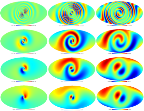
Figure 1: Bianchi patterns in type VII_h models for $x=0.1,\,0.5,\,1,\,5$ (from top to bottom) and $\Omega_{0}=0.1,\,0.5$ and $0.9$ (from left to right). In low density models, the pattern is mostly focused in one hemisphere but for nearly flat models the spiral patterns widen and extend to both hemispheres.

IV Unveiling Hidden Patterns of Bianchi VII_h

Recently Bianchi VII_h models were compared to the first-year WMAP data on large scales and it was shown that the best fit Bianchi model corresponds to a highly hyperbolic model ($\Omega_{0}=0.5$) with a right-handed vorticity $(\frac{\omega}{H})_{0}=4.3\times 10^{-10}$ (Jaffe et al., 2005). There are several aspects to this hidden pattern which should be mentioned. First of all, the proposed model is an extremely hyperbolic model and does not agree with the location of the first peak in the best fit power spectrum of the CMB. In the regime of VII_h models, one should study the nearly flat models in order to have a consistent angular power spectrum. But the problem is that as it has been shown in Fig. 1, the spiral patterns in high density models are not concentrated in one hemisphere and can’t be used to cure the large-scale power asymmetry in the WMAP data reported by Eriksen et al. (2004a).

Second is that the Bianchi patterns we studied so far, are only valid for a matter dominated universe. Patterns must be recalculated in a universe with a dark energy component if one wants to compare them with the observed CMB data which is believed to be there in a $\Lambda$ dominated universe. These issues are addressed in great details by Jaffe et al. (2005b) and they conclude that the “best-fit Bianchi type VII_h model is not compatible with measured cosmological parameters”.

For these reasons, we study the type VII_h Bianchi models only as hidden patterns in the CMB anisotropy maps. We pay our attention to the specific model proposed by Jaffe et al. (2005) and in the next two sections, we address the question whether and to what extent one would be able to discover this pattern and other hidden anisotropic patterns in the CMB anisotropy maps. We carry out our analysis on full sky CMB maps. It has been shown in our previous papers Hajian & Souradeep (2005), that for a masked CMB sky maps, the Bipolar power spectrum has a calculable specific form. In that case, the violation of SI is measured with respect to the ‘bias’ that arises for the masked sky map. The excess BiPS signature would certainly depend to some extent on the specific orientation of the Bianchi template in the sky, given by the extent to which the pattern is covered by the mask. In this work we choose to keep our analysis independent of the orientation of the hidden pattern.

Bipolar Power Spectrum Analysis

We choose a Bianchi VII_h model with $\left(\frac{\sigma_{12}}{H}\right)_{0}=\left(\frac{\sigma_{13}}{H}\right)_{0}=\left(\frac{\sigma}{H}\right)_{0}$. The temperature fluctuations induced by this model are given by eqn. (III) and will be

$$\frac{\Delta T(\theta_{0},\phi_{0})}{T_{0}}=\left(\frac{\sigma}{H}\right)_{0}[A(\theta_{0}) + B(\theta_{0})]\sin{\phi_{0}}$$ (23)

$$+\,\,[B(\theta_{0}) - A(\theta_{0})]\cos{\phi_{0}},$$

Power spectrum of the above Bianchi-induced fluctuations can be computed analytically (Barrow et al., 1985; McEwen et al., 2005b) and is given by

$$C_{l}=\frac{4\pi^{2}}{2l+1}\left(\frac{\sigma}{H}\right)_{0}^{2}[(I_{l}^{A})^{2}+(I_{l}^{B})^{2}],$$ (24)

where

$$I_{l}^{A} = \sqrt{\frac{2l+1}{4\pi l(l+1)}}\int_{0}^{\pi}{A(\theta)P_{l}^{1}(\cos{\theta})\sin{\theta}\rm{d}\theta}$$ (25)

$$I_{l}^{B} = \sqrt{\frac{2l+1}{4\pi l(l+1)}}\int_{0}^{\pi}{B(\theta)P_{l}^{1}(\cos{\theta})\sin{\theta}\rm{d}\theta}$$

The majority of the power in this Bianchi template is contained in multipoles below $l\sim 20$. Therefor to study this particular model we do not need high resolution CMB anisotropy maps.

To do a statistical study of the Bianchi patterns, we generate the pattern for a given model. This pattern is given by the shear components, $x$ parameter and the $\Omega_{0}$. We will then simulate random CMB maps from the best fit $C_{l}$ of the WMAP data (Spergel et al., 2003). We add these two maps with a strength factor $\alpha$ which will let us control the relative strength of the pattern and the random map (see Fig. 2). The resultant map is then given by

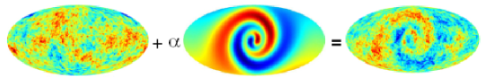
Figure 2: Adding a pattern template with a strength $\alpha$ to a random realization of the CMB anisotropy map. This introduces a preferred direction in the map and violates the statistical isotropy. Maps are rotated to place the Galactic pole at the center for clear illustration.

$$\Delta T(\hat{n})\,=\,\Delta T^{CMB}(\hat{n})+\alpha\Delta T^{Bianchi}(\hat{n}),$$ (26)

and hence the power spectrum of this map will be given by

$$C_{l}=C_{l}^{CMB}+\alpha^{2}C_{l}^{Bianchi}$$ (27)

$\alpha$ is related to $(\frac{\sigma}{H})_{0}$ through $(\frac{\sigma}{H})_{0}$ =$\frac{\alpha}{T_{0}}$ where $T_{0}=2.73\times 10^{6}\mu K$.

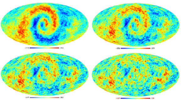
Figure 3: Four Bianchi added CMB maps with different strength factors, rotated to place the Galactic pole at the center for clear illustration. The Bianchi template in the above maps has been computed with $x=0.55,\,\Omega_{0}=0.5$ and strength factors $(\frac{\sigma}{H})_{0}=1.83\times 10^{-9}$ (top left), $(\frac{\sigma}{H})_{0}=1.09\times 10^{-9}$ (top right), $(\frac{\sigma}{H})_{0}=7.3\times 10^{-10}$ (bottom left), $(\frac{\sigma}{H})_{0}=3.66\times 10^{-10}$ (bottom right). Although the pattern can hardly be seen in the fourth map, it has a considerable non-zero bipolar power spectrum (see Fig 4).

We compute the bipolar power spectrum (BiPS) for the Bianchi added CMB anisotropy maps generated above. The unbiased estimator of BiPS is given by,

$$\kappa_{\ell}=\sum_{ll^{\prime}M}W_{l}W_{l^{\prime}}|\sum_{mm^{\prime}}a_{lm}a_{l^{\prime}m^{\prime}}\mathcal{C}^{\ell M}_{ll^{\prime}}|^{2}-{\mathcal{B_{\ell}}},$$ (28)

where $W_{l}$ is the window function in harmonic space, ${\mathcal{B_{\ell}}}$ is the bias that arises from the SI part of the map and is given by the angular power spectrum, $C_{l}$ and $\mathcal{C}^{\ell M}_{ll^{\prime}}$ are Clebsch-Gordan coefficients. Bipolar power spectrum is zero for statistically isotropic maps and has been studied in great details in Hajian & Souradeep (2005) and Basak et al. (2006). Although BiPS is quartic in $a_{lm}$, it is designed to detect SI violation and not non-Gaussianity (Hajian & Souradeep, 2003b, 2005, 2006). Since BiPS is orientation independent (Hajian & Souradeep, 2005), we do not need to worry about the relative orientation between the background map and the Bianchi template. For different strength factors we simulate 100 Bianchi added CMB maps at HEALPix resolution of $N_{side}=32$ corresponding to $l_{max}=95$. Some of these maps are shown in Figure 3. BiPS of each map is obtained from the total $a_{lm}$ which according to eqn. (26) are $a_{lm}=a^{CMB}_{lm}+\alpha\,a^{Bianchi}_{lm}$. We compute the BiPS for each map using the estimator given in eqn. (28). We average these 100 BiPS and compute the dispersion in them. The dispersion is an estimate of $1\sigma$ error bars. At last we use the total angular power spectrum given in eqn. (27) to estimate the bias. We use the best fit theoretical power spectrum from the WMAP analysis, Spergel et al. (2003), as $C_{l}^{CMB}$ in computing the bias. Some results of BiPS for different strength factors are shown in Figure 4. As it has been discussed in Hajian & Souradeep (2003b, 2005), we can use different window functions in harmonic space, $W_{l}$, in order to concentrate on a particular $l$-range. This is proved to be a useful and strong tool to detect deviations from SI using BiPS method. In other words, multipole space windows that weigh down the contribution from the SI region of the multipole space will enhance the signal relative to the cosmic error. We use simple filter functions in $l$ space to isolate different ranges of angular scales; low pass, Gaussian filters

$$W_{l}^{G}=N^{G}\exp\left\{-\left(\frac{2l+1}{2l_{s}+1}\right)^{2}\right\}$$ (29)

that cut power on scales $(l\geq l_{s})$ and band pass filters of the form

$$W_{l}^{S}=2N^{S}\left[1-J_{0}\left(\frac{2l+1}{2l_{s}+1}\right)\right]\exp\left\{-\left(\frac{2l+1}{2l_{s}+1}\right)^{2}\right\},$$ (30)

where $J_{0}$ is the ordinary Bessel function and $N^{G}$ and $N^{S}$ are normalization constants chosen such that,

$$\sum_{l}\frac{(2l+1)W_{l}}{2l(l+1)}=1$$ (31)

i.e., unit rms for unit flat band angular power spectrum $C_{l}=\frac{2\pi}{l(l+1)}$.

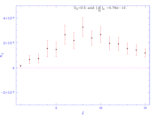
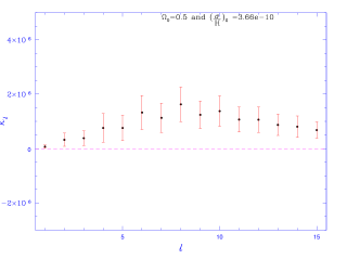
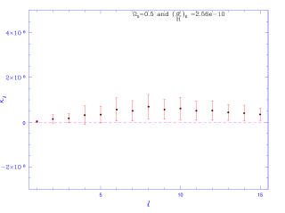
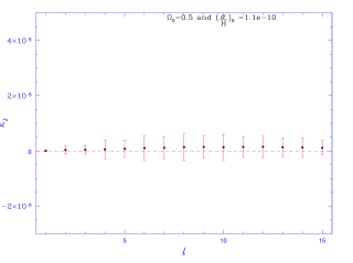
Figure 4: Bipolar power spectrum of Bianchi added CMB maps with strength factors of $(\frac{\sigma}{H})_{0}=4.76\times 10^{-10},3.66\times 10^{-10},2.56\times 10^{-10},1.25\times 10^{-10}$. We have used $W_{l}^{S}(4,13)$ to filter the maps in order to focus on the low-$l$ (large angular scale) properties of the maps.

We use a simple $\chi^{2}$ statistics to compare our BiPS results with zero,

$$\chi^{2}=\sum_{l=0}^{l_{max}}\left(\frac{\kappa_{l}}{\sigma_{\kappa_{l}}}\right)^{2}.$$ (32)

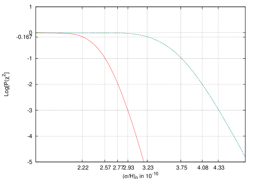
Figure 5: Probability distribution of $\chi^{2}$ versus the shear for $\Omega_{0}=0.5$ Bianchi template. Results of two different window functions, $W_{l}^{G}(25)$ (blue line) and $W_{l}^{S}(4,13)$ (red, solid line) are shown. By testing statistical isotropy of Bianchi embedded CMB maps, we can put a limit of $(\frac{\sigma}{H})_{0}\leq 2.77\times 10^{-10}(99\%CL)$ on Bianchi VII_h models.

The probability of detecting a map with a given BiPS is then given by the probability distribution of the above $\chi^{2}$. Probability of $\chi^{2}$ versus the shear factor is plotted in Figure 5. Being on the conservative side we can constrain the shear to be $(\frac{\sigma}{H})_{0}<2.77\times 10^{-10}$ at a 99% confidence level.

V Conclusion

Bianchi templates, the characteristic temperature patterns in CMB, are imprinted by the unperturbed anisotropic expansion and have preferred directions which violate statistical isotropy of the CMB anisotropy maps. In this paper we study the consistency of the existence of a hidden Bianchi template in the WMAP data that has proposed in recent literature with the previous detection of null bipolar power spectrum in the WMAP first year maps (Hajian et al., 2004). We compute the bipolar power spectrum for low density Bianchi VII_h models embedded in background CMB anisotropy maps with the power spectrum that best fits the first year data of WMAP. We find non-zero bipolar power spectrum for models with $(\frac{\sigma}{H})_{0}\leq 2.77\times 10^{-10}$. This is inconsistent with the null bipolar power spectrum of the WMAP data at $(99\%CL)$. We conclude that correcting the WMAP first year maps for the Bianchi template may make some anomalies in the WMAP data vanish but this will be done at the expense of introducing other anomalies such as preferred directions and violation of statistical isotropy into the Bianchi corrected maps.