Extinction techniques and impact on dust property determination

Abstract

The near infrared extinction powerlaw index ($\beta$) and its uncertainty is derived from three different techniques based on star counts, colour excess and a combination of them. We have applied these methods to 2MASS data to determine maps of $\beta$ and near infrared extinction of the small cloud IC 1396 W. The combination of star counts and colour excess results in the most reliable method to determine $\beta$. It is found that the use of the correct $\beta$-map to transform colour excess values into extinction is fundamental for column density profile analysis of clouds. We describe how artificial photometric data, based on the model of stellar population synthesis of the Galaxy (Robin et al. 2003A&A…409..523R (2003)), can be used to estimate uncertainties and derive systematic effects of the extinction methods presented here. We find that all colour excess based extinction determination methods are subject to small but systematic offsets, which do not affect the star counting technique. These offsets occur since stars seen through a cloud do not represent the same population as stars in an extinction free control field.

1 Introduction

Dust plays a major role in the dynamics of star formation. The determination of its properties and distribution is hence a major challenge towards a better understanding. There are two widely used methods (star counts and colour excess) to determine the distribution and column density of dust in the interstellar medium.

The original idea of using star counts to measure dust extinction dates back to Wolf 1923AN….219..109W (1923). Later Bok 1956AJ…..61..309B (1956) improved the accuracy by implementing star counts at the completeness limit of the images. The difference between the measured and intrinsic colour of a star (colour excess) was used by Lada et al. 1994ApJ…429..694L (1994) to determine the extinction. This approach was optimised by Lombardi & Alves 2001A&A…377.1023L (2001) from multi-band photometry. Recently Lombardi 2005A&A…438..169L (2005) investigated how the two methods can be optimally combined.

Star counts gauge extinction at a given wavelength. The colour excess requires the knowledge of the reddening law to obtain an extinction measurement. Further the reddening law is required to transform these values into the widely used optical extinction ($A_{\rm V}$). This transformation law is not known a priori. There is reasoning that a universal extinction law is valid for the diffuse interstellar medium (Draine 2003ARA&A..41..241D (2003)). In translucent and dense regions, however, processes like coagulation of dust grains and mantle growth can lead to a change in the dust properties (Whittet et al. 2001ApJ…547..872W (2001); Cambrésy et al. 2001A&A…375..999C (2001); del Burgo et al. 2003MNRAS.346..403D (2003); del Burgo & Laureijs 2005MNRAS.360..901D (2005)), which could result in a different extinction law (Larson & Whittet 2005ApJ…623..897L (2005)). Ultraviolet and cosmic ray radiation has also some influence in the density and properties of dust grains (e.g. del Burgo & Cambrésy 2006MNRAS.inprep.D (2006)). Froebrich et al. 2005A&A…432L..67F (2004) showed that the near infrared extinction powerlaw index ($\beta$) within dark clouds can vary significantly from the value obtained for the diffuse interstellar medium.

The purpose of the present paper is the following. We describe an easy-to-use and fast method to determine $\beta$ from multi-filter broad-band observations (Sect. 2). This method is applied in Sect. 3 to an example cloud (IC 1396 W). We discuss the implications of using the determined $\beta$ instead of the standard value of 1.85 (Draine 2003ARA&A..41..241D (2003)), for density profile analyses of dark clouds. In Sect. 4 we present a technique to test the accuracy of extinction determination methods by artificial photometric catalogues based on the model of stellar population synthesis of the Galaxy by Robin et al. 2003A&A…409..523R (2003). We finally discuss systematic uncertainties introduced into extinction maps when using colour excess methods (Sect. LABEL:distcorr). Our conclusions are then put forward in Sect. LABEL:conclusions.

2 Determination of the NIR extinction power law index

There are several possible methods to determine the near infrared extinction power law index ($\beta$). In this section we describe techniques based on star counts, colour excess and a combination of both. The description is done in a general way, in order to adapt the procedure to different datasets. We discuss in detail the uncertainties of each method.

2.1 General notes

Each method discussed below will determine $\beta$ as a function of two variables $(u,v)$. Those can be extinction and/or colour excess. Hence we can write $\beta=f(u,v)$. Each variable consists of $N$ different values (pixels in the extinction and/or colour excess maps). Following Taylor, we describe the difference of the individually measured $\beta$ values from the mean value as:

$$\beta_{i}-\bar{\beta}=(u_{i}-\bar{u})\frac{\partial{\beta}}{\partial{u}}+(v_{i}-\bar{v})\frac{\partial{\beta}}{\partial{v}}$$ (1)

A possible estimator of the variance of $\beta$, defined as

$$\sigma^{2}_{\beta}\equiv\frac{1}{N-1}\sum\limits^{N}_{i=1}(\beta_{i}-\bar{\beta})^{2}$$ (2)

can thus be expressed by the following equation:

$$\sigma^{2}_{\beta}=\sigma^{2}_{u}\left(\frac{\partial{\beta}}{\partial{u}}\right)^{2}+\sigma^{2}_{v}\left(\frac{\partial{\beta}}{\partial{v}}\right)^{2}+2\sigma_{uv}\left(\frac{\partial{\beta}}{\partial{u}}\right)\left(\frac{\partial{\beta}}{\partial{v}}\right).$$ (3)

$\sigma^{2}_{u}$ and $\sigma^{2}_{v}$ refer to the estimators of the variance of the variables $(u,v)$. They can be estimated as the square of the noise in the input extinction and/or colour excess maps. The estimator of the covariance of the two input variables

$$\sigma_{uv}\equiv\frac{1}{N-1}\sum\limits^{N}_{i=1}(u_{i}-\bar{u})(v_{i}-\bar{v})$$ (4)

can be determined from the extinction and/or colour excess maps as follows: multiply both images and determine the mean pixel value of the product image in an extinction free region. Note that in an extinction free field the mean values $\bar{u}$ and $\bar{v}$ are zero.

In the next three subsections we introduce three different methods to determine the function $\beta=f(u,v)$ and the resulting estimator of the variance ($\sigma^{2}_{\beta}$).

2.2 Star Counts

Extinction mapping using accumulative star counts allows us to determine the extinction at wavelength $\lambda$ where the photometry is obtained (e.g. Wolf 1923AN….219..109W (1923); Cambrésy et al. 2002AJ….123.2559C (2002); Froebrich et al. 2005A&A…432L..67F (2004)). It is assumed that extinction has been measured with two different filterbands at reference wavelengths ($\lambda_{1}<\lambda_{2}$). Also we assume the extinction has a power-law dependence $A_{\lambda}\propto\lambda^{-\beta}$ in the wavelength range of interest. Then, the unknown index $\beta$ can be determined from:

$$\beta=\frac{\ln(A_{\lambda_{1}}/A_{\lambda_{2}})}{\ln(\lambda_{2}/\lambda_{1})}.$$ (5)

To estimate the uncertainty of $\beta$ we introduce two parameters: 1) $\alpha_{\rm sc}$, which corresponds to the ratio of the estimators of the variance in the two star count maps, i.e. $\alpha_{\rm sc}\equiv\sigma^{2}_{A_{\lambda_{1}}}/\sigma^{2}_{A_{\lambda_{2}}}$ 2) $\gamma_{\rm sc}$, which corresponds to the ratio of the estimator of the variance in the star count map at $\lambda_{1}$ and the estimator of the covariance of the two star count maps, i.e. $\gamma_{\rm sc}\equiv\sigma^{2}_{A_{\lambda_{1}}}/\sigma_{A_{\lambda_{1}}A_{\lambda_{2}}}$. The estimator of the variance of $\beta$ can then be expressed as:

$$\sigma^{2}_{\beta}=\frac{1}{\ln^{2}\left(\lambda_{2}/\lambda_{1}\right)}\frac{\sigma^{2}_{A_{\lambda_{1}}}}{A^{2}_{\lambda_{1}}}\left[1+\frac{1}{\alpha_{\rm sc}}\left(\frac{\lambda_{2}}{\lambda_{1}}\right)^{2\beta}-\frac{2}{\gamma_{\rm sc}}\left(\frac{\lambda_{2}}{\lambda_{1}}\right)^{\beta}\right]$$ (6)

Figure 1 (top-left) shows, as an example, the relative uncertainty $\Delta\beta/\beta=\sqrt{\sigma^{2}_{\beta}}/\beta$ versus $\beta$ for typical star counts in J- and H-band 2MASS data. The three different lines in Fig. 1 (top-left) denote extinction measurements $A_{\rm J}$ of 4, 6 and 10$\sigma$. For 2MASS data in the area of IC 1396 W we have determined $\alpha_{\rm sc}=1.4$ and $\gamma_{\rm sc}=1.4$ (see below). It is found that a high accuracy for the extinction measurements is required to obtain a good signal to noise ratio (S/N) for $\beta$; for typical values of $\beta=1.4$ at least a $4\sigma$ detection of the extinction in the J-band is needed to determine $\beta$ with an accuracy of 40 %. Note that this is valid for a single measurement only (1 independent pixel in the extinction map). The S/N can be improved by averaging over several independent measurements (see below).

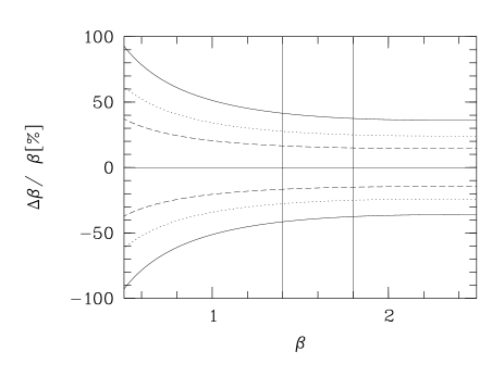
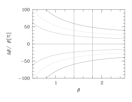
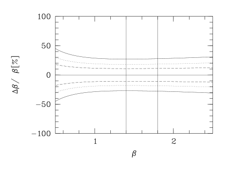
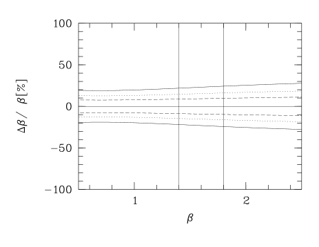
Figure 1: Top-left: Relative uncertainty of $\beta$ obtained from J- and H-band star counts. Top-right: Relative uncertainty of $\beta$ obtained from $\left<J-H\right>$ and $\left<H-K\right>$ colour excess ratio. Bottom: Relative uncertainty of $\beta$ obtained from the combination of J-band star counts and $\left<J-H\right>$ colour excess. The plots show $\Delta\beta/\beta$ referring to measurements of $A_{\rm J}$ (left panels) and $\left<J-H\right>$ (right panels) with a S/N of 4 (solid line), 6 (dotted line), and 10 (dashed line). Values of $\alpha_{\rm sc}=1.4$, $\gamma_{\rm sc}=1.4$, $\alpha_{\rm cosc}=13$, $\gamma_{\rm cosc}=6.5$, $\alpha_{\rm co}=3.6$ and $\gamma_{\rm co}=3.7$ were used for the determination (see text for details). The two vertical lines in the plots indicate values of $\beta=1.4$ and 1.8, which represent the value for dense regions and the diffuse ISM, respectively. Note that the two bottom panels are identical despite showing apparently different behaviour. The relative uncertainty of $\beta$ as a function of the S/N in the $A_{\rm J}$ map (Eq. 13) can be converted into the relative uncertainty of $\beta$ as a function of the S/N in the $\left<J-H\right>$ map using Eq. 12 and the values of $\alpha_{\rm cosc}$ and $\gamma_{\rm cosc}$.

2.3 Colour excess

The most simple approach of a colour excess method is to measure the apparent brightness of a star at two different wavelengths, $m_{\lambda_{1}}$ and $m_{\lambda_{2}}$, and compare the colour $m_{\lambda_{1}}$ - $m_{\lambda_{2}}$ with the theoretical value for main sequence stars or the colour of stars measured in an extinction free control field $m^{\rm tr}_{\lambda_{1}}$ - $m^{\rm tr}_{\lambda_{2}}$ (e.g. Lada et al. 1994ApJ…429..694L (1994)). The colour excess $\left<\lambda_{1}-\lambda_{2}\right>$ is defined as:

$$\left<\lambda_{1}-\lambda_{2}\right>\equiv\left(m_{\lambda_{1}}-m_{\lambda_{2}}\right)-\left(m^{\rm tr}_{\lambda_{1}}-m^{\rm tr}_{\lambda_{2}}\right)$$ (7)

If we assume that this colour excess is entirely due to extinction and, as for the star count analysis, a constant $\beta$ is valid, we can determine the extinction at $\lambda_{2}$ by

$$A_{\lambda_{2}}=\frac{\left<\lambda_{1}-\lambda_{2}\right>}{\left(\frac{\lambda_{2}}{\lambda_{1}}\right)^{\beta}-1}.$$ (8)

Measuring $\left<\lambda_{2}-\lambda_{3}\right>$, with $\lambda_{1}<\lambda_{2}<\lambda_{3}$, we as well can determine the extinction at $\lambda_{2}$:

$$A_{\lambda_{2}}=\frac{\left<\lambda_{2}-\lambda_{3}\right>}{1-\left(\frac{\lambda_{3}}{\lambda_{2}}\right)^{-\beta}}$$ (9)

The right hand side of both equations should essentially give the same value. We can define the colour excess ratio $R\equiv\frac{\left<\lambda_{1}-\lambda_{2}\right>}{\left<\lambda_{2}-\lambda_{3}\right>}$ and obtain the following equation for $\beta$:

$$0=\left(\frac{\lambda_{2}}{\lambda_{1}}\right)^{\beta}+R\cdot\left(\frac{\lambda_{3}}{\lambda_{2}}\right)^{-\beta}-R-1$$ (10)

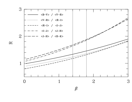
Figure 2: Solution of Eq. 10 for a number of common filter/wavelength combinations. This plot allows us to estimate $\beta$ from the ratio of the colour excess of the two shorter and the two longer wavelength. We plot: BVR (solid), VRI (dotted), RIJ (short-dash), IJH (dash-dot) and JHK (long-dash).

Fig. 2 shows the solution of Eq. 10 for some filter combinations. These plots allow us to estimate $\beta$ for a certain filterband combination and measured colour excess ratio.

Since $\beta$ cannot be determined analytically from Eq. 10, we assume that $\beta={\bf B}(R)$ provides a solution of Eq. 10 with sufficient accuracy (the function ${\bf B}(R)$ could be a polynomial of order $n$). Then we can determine the estimator of the variance of $\beta$ using:

$$\sigma^{2}_{\beta}=\frac{\sigma^{2}_{\left<\lambda_{1}-\lambda_{2}\right>}}{\left<\lambda_{1}-\lambda_{2}\right>^{2}}R^{2}\left[1+\left(\frac{R}{\alpha_{\rm co}}\right)^{2}-2\frac{R}{\gamma_{\rm co}}\right]\left(\frac{\partial{\bf B}(R)}{\partial R}\right)^{2}$$ (11)

Note that the partial derivative $\partial{\bf B}(R)/\partial R$ can directly be obtained from Eq. 10 by using the inverse function theorem. We define the parameters $\alpha_{\rm co}\equiv\sigma^{2}_{\left<\lambda_{1}-\lambda_{2}\right>}/\sigma^{2}_{\left<\lambda_{2}-\lambda_{3}\right>}$ and $\gamma_{\rm co}\equiv\sigma^{2}_{\left<\lambda_{1}-\lambda_{2}\right>}/\sigma_{\left<\lambda_{1}-\lambda_{2}\right>\left<\lambda_{2}-\lambda_{3}\right>}$. Average values based on 2MASS data for IC 1396 W are $\alpha_{\rm co}=3.6$ and $\gamma_{\rm co}=3.7$. Note that these values depend on the intrinsic scatter of the stellar colours, the spacial distribution of stars and the photometric uncertainties in the data, and are hence subject to change slightly with position. In Fig. 1 (top-right) the resulting relative uncertainty of $\beta$ for this example is plotted. Similar to the star counting technique, high S/N colour excess maps are required to reliably estimate $\beta$. We note, however, that for the same dataset usually a higher S/N is achieved for the colour excess method than for the star counting (see e.g. Cambrésy et al 2002AJ….123.2559C (2002)).

2.4 Combining star counts and colour excess

If observations at only two wavelengths $\lambda_{1}<\lambda_{2}$ are available, we do not necessarily need to determine $\beta$ solely from star counts. We can combine star counts and colour excess. If we measure the extinction $A_{\lambda_{1}}$ by star counts, the colour excess $\left<\lambda_{1}-\lambda_{2}\right>$, and assume that $\beta$ is constant in the wavelength range of interest, then $\beta$ can be determined as:

$$\beta=-\ln\left(1-\frac{\left<\lambda_{1}-\lambda_{2}\right>}{A_{\lambda_{1}}}\right)/\ln\left(\lambda_{2}/\lambda_{1}\right)$$ (12)

As for the other two methods, we can estimate the uncertainty associated to the procedure. Similar to those we define the parameters $\alpha_{\rm cosc}\equiv\sigma^{2}_{A_{\lambda_{1}}}/\sigma^{2}_{\left<\lambda_{1}-\lambda_{2}\right>}$ and $\gamma_{\rm cosc}\equiv\sigma^{2}_{A_{\lambda_{1}}}/\sigma_{A_{\lambda_{1}}\left<\lambda_{1}-\lambda_{2}\right>}$, and obtain the estimator of the variance of $\beta$:

$$\begin{gathered}\sigma^{2}_{\beta}=\frac{1}{\ln^{2}\left(\lambda_{2}/\lambda_{1}\right)}\frac{\sigma^{2}_{A_{\lambda_{1}}}}{A^{2}_{\lambda_{1}}}\left(\frac{\lambda_{2}}{\lambda_{1}}\right)^{2\beta}\hskip 105.2751pt\\ \hskip 7.11317pt\cdot\left\{\left[1-\left(\frac{\lambda_{2}}{\lambda_{1}}\right)^{-\beta}\right]^{2}+\frac{1}{\alpha_{\rm cosc}}-\frac{2}{\gamma_{\rm cosc}}\left[1-\left(\frac{\lambda_{2}}{\lambda_{1}}\right)^{-\beta}\right]\right\}\end{gathered}$$ (13)

Figure 1 (bottom) shows two examples of the relative uncertainty of $\beta$ when determined from the combination of star counts and colour excess. Both cases combine J-band star counts and $\left<J-H\right>$ colour excess. In Fig. 1 (bottom left) J-band star counts are used as a measure of the S/N. In Fig. 1 (bottom right) the $\left<J-H\right>$ colour excess is used. Values of $\alpha_{\rm cosc}=13$ and $\gamma_{\rm cosc}=6.5$ are obtained for the example (IC 1396 W).

2.5 Other combinations

If observations at three wavelengths are available and we assume that there is a constant $\beta$, in principle a variety of other possible combinations of colour excess and star counts emerges. One can combine colour excess between two of the wavelengths with star counts at a third wavelength. Also two other combinations using purely colour excess are possible. Since the procedure for the determination of $\beta$ and its uncertainty, as well as the results are very similar to the techniques described in the above paragraphs, we refrain from presenting them here.

2.6 Usage of broad-band filters

The analysis so far is implicitly carried out using the simplifying assumption that extinction and colour excess measurements are carried out at monochromatic wavelengths. Usually the observations are, however, obtained using broadband filters. Does this influence our results?

Firstly we note that extinction and colour excess measurements are obtained by averaging data over a number stars in a certain area. For example the colour excess maps of IC 1396 W (presented below) are determined using on average 25 stars at each position. The average spectral energy distribution of these stars indeed will change the reference wavelength of the used filter. For NIR observations, as used here, the reference wavelength will be shorter as the reference wavelength of the used filter. Second we note that all determination procedures for $\beta$ and its uncertainty depend on the ratio of two wavelength. A change of this ratio would imply systematic off-sets in our determined $\beta$-value. Since for all NIR filters the shift in reference wavelength is toward shorter wavelength, the resulting change in the wavelength ratio will be small.

To estimate this we have convolved black body curves with temperatures between 2000 K and 12000 K with 2MASS filter profiles. It is found that the resulting shift in the reference wavelength ratio is at most 0.5 %. This generally results in about 3 % systematic off-sets for the value of $\beta$. It is hence much smaller than the determined statistical noise, which is in the order of 30 % or higher. Thus, the use of broad band filters does not influence our results.

2.7 Discussion

In general all methods described here have similar uncertainties when applied to the same wavelength range. But it is possible to determine the method leading to the highest S/N in $\beta$ for any particular dataset. However, there might be additional systematic uncertainties (see Sect. LABEL:distcorr for a discussion). Figure 1 allows us to compare the different methods. In the left panels the relative uncertainties of $\beta$ are plotted as a function of the S/N in the J-band star count map. Note that for purely star counting the uncertainties are larger as for the combination of star counts and colour excess. In the right panels of Fig. 1 the relative uncertainties of $\beta$ as a function of the S/N in the $\left<J-H\right>$ colour excess map are plotted. We find that the scatter is smaller when combining colour excess and star counts instead of using the colour excess ratio. This is especially the case towards smaller values of $\beta$. We conclude that for our example (IC 1396 W) the combination of J-band star counts and $\left<J-H\right>$ colour excess provides the best $\beta$-map. Note that this might change for other datasets, since the estimator of the variance of $\beta$ depends on the values of $\alpha_{\rm i}$ and $\gamma_{\rm i}$.

Even when using the best method to determine $\beta$, the uncertainties based on individual measurements (one independent pixel in the extinction/colour excess maps) are rather large even for high S/N extinction data. However, several pixels may be averaged to decrease the uncertainties. Although a simple averaging over adjoining pixels would decrease the spatial resolution it is in general a good approach in regions were no apparent changes of $\beta$ are seen in the data (i.e. the scatter of $\beta$-values is consistent with the statistical expectations; 68 % of the data points are within the 1$\sigma$ error bars, etc.). If a dependency of $\beta$ on the column density is found (as for IC 1396 W, see below), we suggest to apply the following method to determine how $\beta$ depends on the column density within individual clouds.

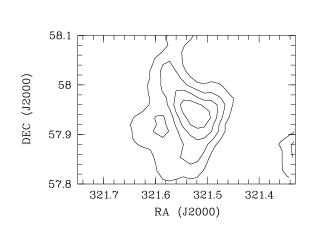
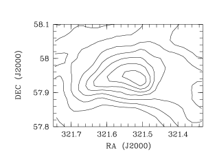
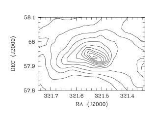
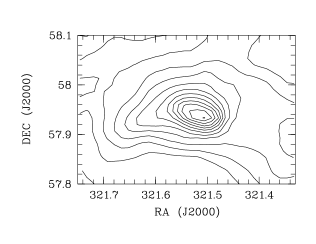
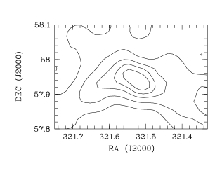
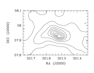
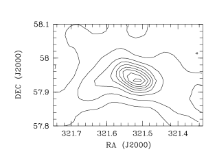
Figure 3: Top: Extinction maps of IC 1396 W obtained from accumulative star counts in 2MASS data. Contours in each panel start at 0.15 mag of extinction in the J-band (left), H-band (middle) and K-band (right) and increase by 0.15 mag with each step. Middle: Extinction maps of IC 1396 W obtained from $\left<J-H\right>$ colour excess in 2MASS data. Contours start at 0.15 mag of extinction in the J-band and increase by 0.15 mag with each step. The conversion of colour excess into extinction uses $\beta=1.8$ (left), the $\beta$-map obtained from the $\left<J-H\right>$ and $\left<H-K\right>$ colour excess ratio (middle) and the best $\beta$-map determined from $\left<J-H\right>$ colour excess and J-band star counts. Bottom: The same as the middle row but for $\left<H-K\right>$ colour excess. Contours are in H-band extinction.

• Accumulated star counts or its combination with colour excess: For each independent pixel $\beta$ is plotted against extinction (e.g. $A_{\lambda_{1}}$). A running mean in this diagram can then be used as representation of the relation $\beta$-$A_{\lambda_{1}}$. Alternatively mean values of $\beta$ in certain $A_{\lambda_{1}}$-bins can be fit by an appropriate function to establish the relation $\beta$-$A_{\lambda_{1}}$.

• Colour excess: The determination of the extinction from colour excess requires the knowledge of $\beta$. Thus, as a first step for each independent pixel the value of $\beta$ is plotted against the colour excess (e.g. $\left<\lambda_{1}-\lambda_{2}\right>$). Similar to the accumulated star count method we establish the relation $\beta$-$\left<\lambda_{1}-\lambda_{2}\right>$ using a running mean or by fitting an appropriate function. This relation then can be used to determine the extinction from the colour excess and to determine e.g. the relation $\beta$-$A_{\lambda_{1}}$.

3 A case study: IC 1396 W

In order to illustrate the $\beta$-determination procedure and its implications on extinction and cloud column density profiles, we present in this section an example, the small cloud IC 1396 W. This object is part of the Cep OB 2 association, about 8’ in size and at roughly 750 pc distance (e.g. Froebrich & Scholz 2003A&A…407..207F (2003)). The position of the cloud in the sky and the 2MASS detection limits facilitate our analysis in the way that there is only a negligible fraction of foreground stars to the cloud. Hence we do not need to remove foreground stars when determining extinction maps.

3.1 Extinction maps

In the top panel of Fig. 3 we show the three extinction maps ($A_{\rm J}$, $A_{\rm H}$, $A_{\rm K}$) for this cloud obtained from accumulative star counts. The contours start at 0.15 mag extinction at the filter wavelength and increase by this amount. The basic structure (central peak and small extension to the East) of the cloud is the same in all three filters. The extinction maps obtained from the colour excess maps show a slightly different structure (see bottom panel of Fig. 3). In particular we can trace much better the outer areas of the cloud. There is an apparent small offset between the star count and colour excess extinction maps. This can be explained by possible differences in the selection of the control field (for the colour excess an apparently IRAS emission free field south of the cloud was chosen, in contrast to the surrounding 1^∘x1^∘ field for the star counts).

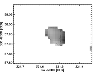
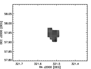
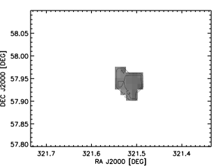
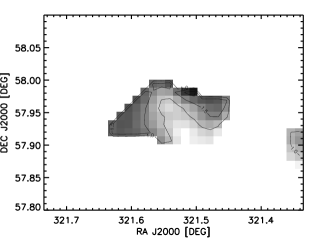
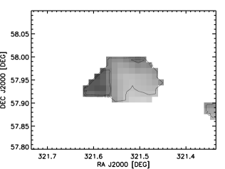
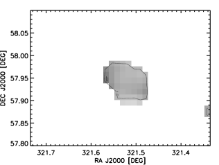
Figure 4: Top: Gray scale $\beta$-maps obtained from accumulative star count extinction maps for the wavelength range JH (left), HK (middle) and JK (right). Bottom left: Gray scale $\beta$-map obtained from $\left<J-H\right>$ and $\left<H-K\right>$ colour excess maps. Bottom middle: $\beta$-map obtained from the combination of $\left<J-H\right>$ colour excess and J-band star counts. Bottom right: Gray scale $\beta$-map obtained from the combination of $\left<H-K\right>$ colour excess and H-band star counts. In all panels only areas with extinction or colour excess values above the 3$\sigma$ noise level are used. Isocontours of $\beta$=1.0 and 1.5 are marked on gray scale maps where darker colours represent higher values of $\beta$.

3.2 $\beta$-maps

In the top panel of Fig. 4 we show the $\beta$-maps of the cloud, as determined from the star counts in JH, HK and JK and using Eq. 5. The bottom left panel of Fig. 4 displays the $\beta$-map obtained from the $\left<J-H\right>$ and $\left<H-K\right>$ colour excess maps and Eq. 10. The two remaining maps are determined using the combination of star counts, colour excess and Eq. 12. In the bottom middle panel we combine J-band star counts with $\left<J-H\right>$ colour excess, and in the bottom right panel H-band star counts and $\left<H-K\right>$ colour excess. In all cases only pixels are shown, where the used extinction or colour excess is 3$\sigma$ above the noise.

The first thing to note is that $\beta$-maps obtained using colour excess cover a larger area, indicating the superiority of the colour excess method to the star count method in the NIR, in terms of S/N in the extinction maps. We also see a structure in the $\beta$-map that agrees well with the structure in the extinction maps. This suggests a dependence of $\beta$ on the column density in this cloud. In the outer regions of the cloud values for $\beta$ close to the canonical value for the interstellar medium of 1.85 (Draine 2003ARA&A..41..241D (2003)) are found. In the centre of the cloud, where extinction is higher, $\beta$ drops to significantly smaller values, partly even below 1.0. When using solely star counts to determine $\beta$ a smaller area is above the $3\sigma$ noise level and no structural information can be obtained. However, the combination of J-band star counts and $\left<J-H\right>$ colour excess agrees very well with the $\beta$-map obtained solely from colour excess. The small offset in the absolute $\beta$-values is due the different control fields used (see discussion above). We note, however, that differences in $\beta$ within a single cloud can be easily determined by our method. The correct absolute value for $\beta$ requires a carefully chosen comparison field, which is free of extinction.

3.3 Column density profile

How does the change of $\beta$ influence column density profiles of the cloud? We plot in Fig. 5 the column density profile (normalised to the peak) from East to West across the cloud at a declination of 57.93^∘. The solid line shows the profile from J-band star counts and the dotted line from $\left<J-H\right>$ colour excess (converted with a constant $\beta$-value). There is a significant difference between the two profiles. The small peak in the East shows a much higher column density relative to the main peak when using colour excess instead of star counts. Note that this difference is unchanged when varying $\beta$, as long as a constant value is used for the whole cloud.

We used our $\beta$-map obtained from the combination of J-band star counts and $\left<J-H\right>$ colour excess to convert the $\left<J-H\right>$-map into column density. The resulting profile is shown in Fig. 5 as dot-dashed line. It is obvious that this dramatically changes the column density profile which now much more closely matches the profile obtained solely from star counts. Note that we obtain the same result when using the $\beta$-map obtained from colour excess only (dashed line).

This example shows that the column density structure of clouds can differ significantly depending on the method used to determine the extinction maps. This in particularly holds when changes of $\beta$ are found within the cloud. Thus, extinction maps from accumulative star counts or colour excess (using the correct $\beta$ values) should be favoured when investigating the structures/profiles of the denser parts of clouds, where changes of $\beta$ are more frequently observed. When investigating the outer areas of clouds, where $\beta$ is very close to the ISM value, or at least constant, colour excess extinction maps provide the better solution due to their higher signal to noise.

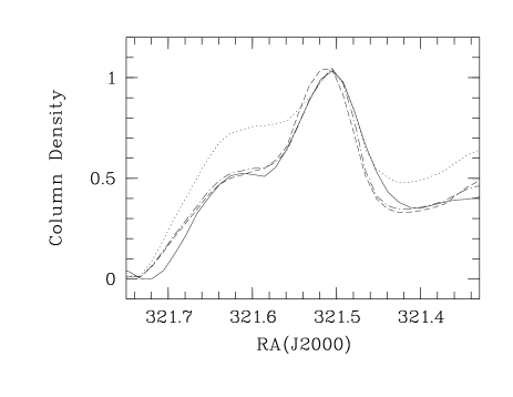
Figure 5: Column density profiles (normalised to zero at the eastern edge of the cloud and unity at the peak) across IC 1396 W at a declination of 57.93^∘. The solid line shows the profile obtained from J-band star counts and the dotted line is based on $\left<J-H\right>$ colour excess and a constant $\beta$. The dash-dot line uses a combination of J-band star counts and $\left<J-H\right>$ colour excess to determine the $\beta$-map, required to convert $\left<J-H\right>$ into extinction. The dashed line is the column density profile when using the $\beta$-map obtained from the $\left<J-H\right>$ and $\left<H-K\right>$ colour excess ratio.

4 Test of extinction determination

Given the possible large uncertainties in the determination of $\beta$, it is worthy to know the uncertainties of the underlying extinction maps from star counts or colour excess determination procedures. In particular any systematic effect should be investigated and corrected for. Here we introduce a scheme to test the reliability of the extinction determination methods. A detailed discussion about the influence of the box size to the measured extinction, systematic offsets in colour excess methods and limitations for reliable foreground star detection is given.

4.1 Artificial data

We used the model of stellar population synthesis of the Galaxy by Robin et al. 2003A&A…409..523R (2003) to generate artificial data. This model allows us to generate artificial photometric catalogues for a given region in the sky. Constraints for the limiting magnitude in each filterband can be applied. We performed all our simulations using 2MASS catalogue magnitude limits (J_max = 16.5, H_max = 16.0, K_max = 15.5). As position we selected ($l$ = 81^∘, $b$ = 0^∘). This coincides with the position of the DR 21 star forming region and hence the quantitative results of this study can be applied for this area. For any other region in the sky only the qualitative part of the analysis can be applied; for quantitative results the simulations described here have to be applied to the specific area.

As mentioned, we determine only the extinction at a certain wavelength when using accumulative star counts, or we can determine the colour excess between two wavelengths. The conversion into optical extinction requires the knowledge of the extinction law. Since we know the extinction law applied to generate the artificial data (Mathis 1990ARA&A..28…37M (1990)), we are able to directly compute the optical extinction. This is what finally is used to estimate the reliability of our extinction determination procedure.

units ¡30mm,30mm¿ point at 0 0 x from -0.5 to 1.5 , y from -0.5 to 1.5 left label ticks in long numbered from -0.5 to 1.5 by 0.5 short unlabeled from -0.5 to 1.5 by 0.1 / right label ticks in long unlabeled from -0.5 to 1.5 by 0.5 short unlabeled from -0.5 to 1.5 by 0.1 / bottom label ticks in long numbered from -0.5 to 1.5 by 0.5 short unlabeled from -0.5 to 1.5 by 0.1 / top label ticks in long unlabeled from -0.5 to 1.5 by 0.5 short unlabeled from -0.5 to 1.5 by 0.1 /

A photometric catalogue with the same magnitude limits and position was downloaded, but this time including a cloud with a certain distance and a certain extinction. Each star in this second catalogue was supplied with artificial, uniformly distributed coordinates, that placed it in the central 1^∘x1^∘ field.

The two catalogues where merged in a way that all stars in the first catalogue which fell in the central 0.5^∘x0.5^∘ area (solid lines in Fig. LABEL:testfield) are replaced by the stars of the second catalogue in this area. In other words we created an artificial catalogue, simulating a squared 0.5^∘x0.5^∘ cloud in the centre of a 2^∘x2^∘ field.

For each of these artificial datasets we determined the extinction map for the central 1^∘x1^∘ field and measured the mean and median extinction of the cloud in the central 0.25^∘x0.25^∘. This set-up allows us to perform different tests to determine the reliability of our extinction determination method.

4.2 Zero extinction (i.e. no clouds)

Here we consider an object with zero extinction at zero distance to estimate the contribution of the simulated photometric datasets and artificial coordinates to the noise of the method. Such an object is equivalent to consider ”no cloud”, but it is also representative of a region with negligible extinction.

We first fix the set of stars in the control field, the cloud and the coordinates assigned to these stars. This allows us to determine how the chosen box size influences the noise in the extinction map. As expected we find that the box size is inversely proportional to the noise, with very small deviations. This can be explained since the noise should be inversely proportional to the square root of the number of stars in each box, and then inversely proportional to the box size. As box size for all subsequent analysis we chose 1.2’, which ensures on average 25 stars per box.

Table 1: Contribution of artificial coordinates and set of stars on the noise in the extinction maps from star counts and colour excess for model clouds with negligible extinction. We show here results for K-band star counts and $\left<H-K\right>$ colour excess methods. The noise is given in magnitudes of $A_{\rm V}$.

	noise from
influences	star counts	colour excess
artificial coordinates	0.15	0.03
set of stars in
control field	0.13	0.05
cloud	0.10	0.04
total noise	0.22	0.07

We have performed several tests in order to disentangle the different components contributing to the noise in the extinction maps. In particular: a) the artificial coordinates of the stars in the field; b) the set of stars in the control field; c) the set of stars in the area of the cloud. The contribution to the noise from each of those three components can be determined from the scatter in the synthetic extinction maps, by varying one component and fixing the other two.

Our results are summarised in Table 1. There we compare the noise (in magnitudes of $A_{\rm V}$, converted using the extinction law of Mathis 1990ARA&A..28…37M (1990)) between K-band star counts and $\left<H-K\right>$ colour excess. We find that the star count method leads to three times larger noise (for our chosen magnitude limits and box size). When using the colour excess method, the set of stars in the control field or the cloud is responsible for most of the scatter. For star counts, however, the artificial coordinates dominate the noise.

4.3 Clouds at zero distance

Since we have established the influence of the simulated star sets and artificial coordinates, we now investigate the changes for different cloud extinction values ($A_{\rm V}$ = 0.0, 0.2, 0.5, 1.0, 3.0, 5.0, 7.0, 10.0 mag). To avoid uncertainties due to foreground stars, the model clouds are placed at zero distance.

We test how the scatter in the extinction map changes with $A_{\rm V}$. Figure LABEL:noiseav shows how the noise in the extinction maps changes with $A_{\rm V}$ of the model cloud. The dashed line corresponds to the colour excess method and the dotted line to the accumulated star counts. For low extinction values, below one mag of $A_{\rm V}$, the measured values agree very well with the estimated values in the above section. This can be explained since such low extinction values only marginally influence the number of stars in each box and therefore the noise in the maps. For larger $A_{\rm V}$-values, however, the scatter increases significantly. This is largely due to the fact that a much lower number of stars is present in each box. When comparing the two methods we find that accumulated star counts lead on average to a three to five times higher noise.

units ¡6mm,43.5mm¿ point at 0 0 x from -0.5 to 11 , y from -0 to 1.1 left label ticks in long numbered from 0.25 to 1.0 by 0.25 short unlabeled from 0. to 1.1 by 0.125 / right label ticks in long unlabeled from 0.25 to 1.0 by 0.25 short unlabeled from 0. to 1.1 by 0.125 / bottom label ticks in long numbered from 0 to 10 by 2 short unlabeled from 0 to 10 by 1 / top label ticks in long unlabeled from 0 to 10 by 2 short unlabeled from 0 to 10 by 1 /

For small extinction values ($A_{\rm V}<1$ mag) the deviations are smaller than 1 $\sigma$. For higher extinction ($A_{\rm V}$ up to 7 mag) we systematically underestimate the extinction by up to 2$\sigma$. For very high column densities ($A_{\rm V}\approx 10$ mag) this effect turns and we overestimate the extinction. Clearly an explanation for this effect is needed. Due to the setup of our test, a contribution from foreground stars can be neglected. For small values of extinction (below 1 mag $A_{\rm V}$) the effect is negligible. This implies the reddening of the stars due to the dust in the cloud itself is the cause of the offsets. When comparing the mean/median colour of stars in the cloud and an extinction free control-field, we have to keep in mind that in both areas stars down to a certain limiting magnitude are detected. We see, however, in these two fields different populations of stars. Stars behind the cloud, detected down to the same limiting magnitude, are on average at a different distance and redder. Thus the mean/median intrinsic colour of stars behind the cloud differs from the mean/median intrinsic colour of stars in the control field. In conclusion all methods using colour excess to estimate extinction are subject to this effect. Even if small for low extinction values it might become significant and systematic for denser regions, changing effectively the clouds column density profile.

units ¡6.4mm,60mm¿ point at 0 0 x from -0.5 to 11 , y from -0.3 to 0.5 left label ticks in long numbered from -0.3 to 0.5 by 0.2 short unlabeled from -0.3 to 0.5 by 0.1 / right label ticks in long unlabeled from -0.3 to 0.5 by 0.2 short unlabeled from -0.3 to 0.5 by 0.1 / bottom label ticks in long numbered from 0 to 10 by 2 short unlabeled from 0 to 10 by 1 / top label ticks in long unlabeled from 0 to 10 by 2 short unlabeled from 0 to 10 by 1 /

Do those offsets have a systematic influence on the determination of $\beta$? One can estimate that the value of $\beta$, determined with or without the correction of the systematic offset, differs by at most 5 %. This is usually much smaller than the scatter of $\beta$ (in the order of 30 % or higher) due to the scatter in the colour excess maps (see e.g. Fig. 1). Only for very high S/N data with a very small internal scatter of $\beta$ these offsets become important.

4.4 Clouds with variable distance

Foreground stars have to be identified and removed from the input catalogue because they influence the correct extinction determination. This is usually done by identifying all stars in the field of the cloud that are much bluer than what would be expected from the extinction of the cloud. The notion is stars behind the cloud are red, stars in front of the cloud are blue. This requires, however, the detection of a significant extinction towards the cloud prior to the foreground star identification. Here we investigate the difficulties for the identification of foreground stars for the star counting and colour excess method.

We analyse how the extinction of our model cloud depends on the distance of the cloud. Distances of 0, 0.1, 0.5, 1, 2, 3, 4 and 5 kpc were considered. In Fig. LABEL:distance we plot how the measured extinction depends on the cloud distance for a 10 and 3 mag $A_{\rm V}$ cloud. Accumulative star counts (solid lines) and colour excess (dashed lines) extinction maps, prior to foreground stars selection, are shown.

There are obvious differences between the two methods. The star counting method shows a steady decline of the measured extinction with increasing cloud distance. For the colour excess method at first only a very small decline with cloud distance is observed. After a certain critical distance, however, the measured extinction drops to zero. This is the distance at which more than half of the stars in the field are foreground to the cloud, and the median colour represent foreground stars. The higher the extinction in the cloud the smaller is the maximum distance up to which a cloud can be detected using colour excess since less background stars are detected in the field.

When investigating distant clouds, it is hence of advantage to use the star count extinction maps for foreground star identification. In our example in Fig. LABEL:distance it is observed that we are not able to identify foreground stars in a 10 mag $A_{\rm V}$ cloud with a distance larger than 2 kpc when using colour excess extinction maps. Conversely, the star counting technique is able to detect this cloud at distances of up to 4 kpc at a 3 $\sigma$ level. For 3 mag $A_{\rm V}$ the critical distance for the colour excess method is 3 kpc, compared to 4 kpc for the star counting technique.

units ¡12mm,4mm¿ point at 0 0 x from -0.5 to 5.5 , y from -1 to 11 left label ticks in long numbered from -0 to 10 by 2 short unlabeled from -0 to 10 by 1 / right label ticks in long unlabeled from -0 to 10 by 2 short unlabeled from -0 to 10 by 1 / bottom label ticks in long numbered from 0 to 5 by 1 short unlabeled from 0 to 5 by 0.5 / top label ticks in long unlabeled from 0 to 5 by 1 short unlabeled from 0 to 5 by 0.5 /

We present a scheme to test the accuracy of extinction determination methods using artificial observational data. This is based on the model of stellar population synthesis of the Galaxy by Robin et al. 2003A&A…409..523R (2003). We show that all extinction determination methods based on colour excess are subject to small but systematic offsets. These are due to the fact that the population of stars seen through a cloud is different from the population of stars in an extinction free control field (even if close by). The resulting offsets, however, can be determined with the knowledge of the cloud position, distance and extinction, as well as the completeness limit of the photometric catalogue. The same scheme allows us to estimate the distance out to which clouds can be detected with star counts and colour excess. Generally, star counts allow us to detect more distant clouds than colour excess. This is particularly useful for the first step of foreground star selection in the case of distant clouds.

Acknowledgements

We would like to thank the anonymous referee for significant comments to improve the paper. D. F. received financial support from the Cosmo-Grid project, funded by the Program for Research in Third Level Institutions under the National Development Plan and with assistance from the European Regional Development Fund. This publication makes use of data products from the Two Micron All Sky Survey, which is a joint project of the University of Massachusetts and the Infrared Processing and Analysis Center/California Institute of Technology, funded by the National Aeronautics and Space Administration and the National Science Foundation.

References

- (1) Bertin, E., Arnouts, S., 1996, A&AS, 117, 393
- (2) Bok, B.J. 1956, AJ, 61, 309
- (3) Cambrésy, L., Beichman, C.A., Jarrett, T.H. & Cutri, R.M. 2002, AJ, 123, 2559
- (4) Cambrésy, L., Boulanger, F., Lagache, G., & Stepnik, B. 2001, A&A, 375, 999
- (5) del Burgo, C., Cambrésy, L. 2006, MNRAS, in press, astro-ph/0603002
- (6) del Burgo, C., Laureijs, R.J. 2005, MNRAS, 360, 901
- (7) del Burgo, C., Laureijs, R.J., Ábrahám, P., & Kiss, C. 2003, MNRAS, 346, 403
- (8) Draine, B.T. 2003, ARA&A, 41, 241
- (9) Froebrich, D., Ray, T.P., Murphy, G.C. & Scholz, A. 2005, A&A, 432, 67
- (10) Froebrich, D., Scholz, A. 2003, A&A, 407, 207
- (11) Joshi, Y.C. 2005, MNRAS, 362, 1259
- (12) Kiss, C,. Tóth, L.V., Moór, A., Sato, F., Nikolic, S., Wouterloot, J.G.A., 2000, A&A, 363, 755
- (13) Lada, C.J., Lada, E.A., Clemens, D.P. & Bally, J. 1994, ApJ, 429, 694
- (14) Larson, K.A., Whittet, D.C.B. 2005, ApJ, 623, 897
- (15) Lombardi, M. 2005, A&A, 438, 169
- (16) Lombardi, M., Alves, J., 2001, A&A, 377, 1023
- (17) Mathis, J. S., 1990, ARA&A, 28, 37
- (18) Robin, A.C., Reylé, C., Derrière, S. & Picaud, S. 2003, A&A, 409, 523
- (19) Vilas-Boas, J.W.S., Myers, P.C., Fuller, G.A., 1994, ApJ, 433, 96
- (20) Whittet, D.C.B., Gerakines, P.A., Hough, J.H., & Shenoy, S.S. 2001, ApJ, 547, 872
- (21) Williams, J.P., de Geus, E.J. & Blitz, L. 1994, ApJ, 428, 693
- (22) Wolf, M. 1923, AN, 219, 109