On vector mode contribution to CMB temperature and polarization from local strings

Abstract

In a recent publication, we used the data from WMAP and SDSS to constrain the primordial perturbations and to predict the B-mode polarization sourced by cosmic string networks. We have been alerted Slosar to the existence of errors in the code Pogosian we used to calculate the Cosmic Microwave Background anisotropies from cosmic strings. Correcting the errors leads to a significant increase in the vector mode contribution to the CMB temperature and polarization anisotropies as well as an overall renormalization of the various string spectra. In these notes we explain the nature of the errors and discuss their implications for previously published constraints on cosmic strings based on this code. The chief change in our results is that our derived limit for the cosmic string tension is strengthened: $G\mu<1.8(2.7)\times 10^{-7}$ at 68 (95)% confidence. We also note that the newly-enhanced vector mode contribution produces a greatly-increased amplitude for B-mode polarization in the CMB which could exceed the B-mode power produced by the lensing of primordial E-mode polarization into B-mode polarization.

I Introduction

Our collaboration has used the data from the Cosmic Microwave Background (CMB) anisotropy and from galaxy surveys to place cosmological limits on the properties of networks of cosmic strings in a series of papers PTWW03 ; PWW04 ; WPW05 . We have recently learned Slosar that the code we used to calculate the cosmic string-sourced CMB anisotropy and primordial power spectra contained several errors, the most important of which was a missing normalization factor in the evaluation of the vector mode power produced by cosmic strings. This latter error alone lead to a factor of $\sim 8$ enhancement in vector-mode power. While revising the vector mode part of the code we also located an overall factor of 2 normalization error in all string spectra. Full details of all corrected errors are given in the Appendix.

The enhancement of the vector modes has implications for the results of our last paper WPW05 , especially for the prediction for the B-mode polarization sourced by strings. The principal result of that work was a constraint on the fractional power that strings can contribute to the CMB temperature anisotropy spectrum. Fortunately, this fraction is mainly constrained by the shape of the string induced CMB spectrum, which did not change considerably as a result of fixing the code. Thus we believe that the bounds derived in our last paper on the parameter we called $f$, the fractional power sourced by cosmic strings, will remain unchanged, and can still be used to derive bounds on the properties of the cosmic string network. Changing the normalization of our curves, after correcting our errors, scales downward our fiducial string tension $\mu_{0}$ by a factor of $1.8$, so that our new fiducial string tension is $G\mu_{0}\approx 1.1\times 10^{-6}$. The provisional limits on $G\mu$ that we derive using this corrected fiducial string tension are then $G\mu<1.8(2.7)\times 10^{-7}$ at 68 (95)% confidence. The limits we placed on cosmic string substructure, parameterized by the string wiggliness, $\alpha_{r}$, were weak at best WPW05 ; that determination should now be disregarded completely. We plan to perform our Markov Chain Monte Carlo analysis again, with the corrected string spectra, using the new three-year WMAP data WMAP3 . Until we finish this analysis, we will use these provisional bounds, which we expect to be at least approximately valid

A simple summary of what has changed in light of correcting these errors is that we now find much greater parity between the power in the vector and scalar modes caused by cosmic strings. Because this reapportionment of perturbation does not significantly alter the shape of the string sourced CMB spectrum and, hence, should not affect the cosmological constraints on the fraction of the total CMB power sourced by cosmic strings, the greater proportion of vector mode power leads to a greatly enhanced prediction for B-mode polarization in the CMB. Even with a smaller string tension, the B-mode power we now predict is a factor of 10 - 20 times as great as reported in our previous work. The factor of two uncertainty reflects our ignorance of cosmic string substructure. Given this enhancement, the B-mode polarization signal for a cosmologically viable network of strings could be the most prominent source for a B-mode signal in the CMB, with an amplitude even greater than is expected from E-to-B lensing. A host of experiments aimed at measuring B-modes with the relevant sensitivity ($\gtrsim 0.01(\mu K)^{2}$ for $100<\ell<2000$) are currently in planning or underway polarization . The prominence of the cosmic string B-mode prediction implies that these experiments provide perhaps the best opportunity for either observing a network of cosmic strings or placing limits on its properties.

II Cosmic Microwave Background Temperature Anisotropy

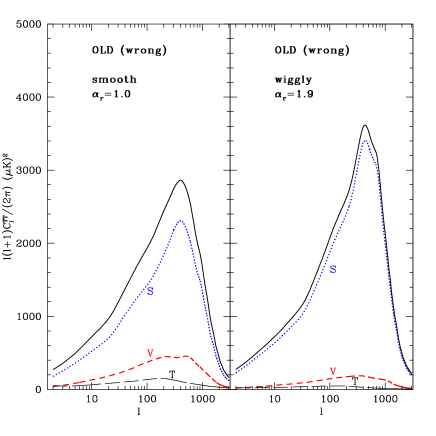
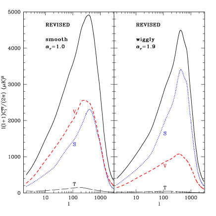
Figure 1: The scalar (blue dot), vector (red short dash), tensor (black long dash) and their sum (solid black) contributions to the CMB TT spectrum evaluated using the old (left) and the revised (right) codes for the cases of smooth ($\alpha_{r}=1$) and wiggly ($\alpha_{r}=1.9$) strings with $G\mu=1.4\times 10^{-6}$. The spectra are proportional to $(G\mu)^{2}$ and this value of $G\mu$ corresponds to the reference cosmic string tension used in our previous work WPW05 , divided by $\sqrt{2}$ (to correct an overall factor of two missing in the power spectra computed from the previous version of our code). Comparing the old and revised plots, it is evident that the new smooth string spectra have a factor of about $1.69$ higher amplitude than the old spectra for the same string tension. We combine these two corrections – a factor of $\sqrt{2}$ in overall normalization and a factor of $\approx\sqrt{1.69}$ from enhanced vector modes – to infer that the correct, fiducial cosmic string tension should be $G\mu_{0}\approx 1.1\times 10^{-6}$, which is a factor of $1.8$ smaller than the fiducial tension estimated in our previous work. The meaning of this fiducial tension, explained in our last paper, is this: $G\mu_{0}$ is the cosmic string tension that would be necessary for a network of cosmic strings to produce the same integrated primordial power as is found in the WMAP best-fit adiabatic model. The parameter $\alpha_{r}$ is the ratio of the effective mass-per-length of a wiggly string to that of a smooth string in the radiation era. See Refs. PV99 ; WPW05 for further details on string substructure.

As discussed in the Appendix, there was an overall factor of $2$ missing in all spectra. One can correct for this factor by dividing the value of the string tension $G\mu_{0}$ by a factor of $\sqrt{2}$. In particular, the value $G\mu_{0}=2\times 10^{-6}$ used in our previous work WPW05 should now be replaced by $G\mu_{0}=1.4\times 10^{-6}$. In addition to this factor of $2$, the enhanced vector-mode power from our corrected code leads to a larger amplitude in the TT spectrum produced by cosmic strings for a given cosmic string tension. In Fig. 1 we show the scalar, vector and tensor contributions to the string-sourced CMB TT spectrum, as well as their sum, before and after correction. We now find that vector modes play a much more prominent role. In the case of smooth strings their contribution is larger than that of scalar modes. This causes the total TT power to be nearly doubled for the same value of $G\mu$. Wiggliness suppresses the vector modes and enhances the scalar modes, a trend already pointed out in Ref. PV99 . The combined effect of wiggliness is to decrease the total TT power as compared with smooth strings. This means that constraints on $G\mu$ are weaker for wiggly strings than for smooth strings. In contrast, our previous work PV99 ; WPW05 reported the erroneous conclusion that wiggliness on strings produce an enhancement of total power and, therefore, a stronger bound on $G\mu$. Thus, the conclusions reported in those papers need to be modified. In particular, the bounds on string wiggliness reported there should be disregarded

It has been accepted among the experts in the field that global strings lead to CMB anisotropies dominated by vector modes while local strings do not. This presumption was, to a degree, based upon the results of previous studies ABR99 ; PV99 , where vector modes were found to be subdominant even for smooth strings. It now appears that this perception was incorrect, at least in the case of smooth strings. However, we do expect local strings to be quite wiggly, since they accumulate small-scale structure over the course of their evolution. Hence, we should still expect vector modes to be relatively low for local strings. Global strings, in contrast, are typically smooth and relativistic, so there is no similar mechanism available to suppress their vector modes.

III B-mode Polarization in the CMB

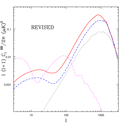
Figure 2: The CMB BB spectra. Left: the plot from our last paper WPW05 showing contributions from inflation for $r=0.1$ (dash-dot), lensing (dot) and cosmic strings (solid line for smooth and dash line for wiggly). Right: revised predictions for the smooth (solid, red) and wiggly (dashed, blue) cases based on the assumption that strings contribute $10$% of the power in the CMB TT spectrum. Inflation and lensing estimates are plotted as in the left hand panel but with the inflationary tensor mode color-coded magenta and E to B lensing still black.

Cosmic string-sourced vector mode perturbations can lead to B-mode polarization in the CMB. In view of the ongoing quest to observe B-type polarization in the CMB polarization , it is of particular interest to revisit the B-mode predictions for cosmic strings made in our previous analysis WPW05 . In that paper we found that approximately $10$% of the observed CMB TT spectrum can be produced by strings (fraction in strings $f_{s}=0.1$). This fraction depends only on the shape of the string induced spectrum, so since the shapes of the old and revised spectra, as shown in Fig. 1, are quite similar, we will assume that $f_{s}=0.1$ is still a valid upper bound.

Let us define $B$ as the coefficient by which one needs to multiply the string TT spectrum in Fig. 1 in order for it to contribute $f_{s}=0.1$. The two spectra shown in Fig. 1 would need different values of $B$ to satisfy this bound. In our previous work WPW05 we determined that $f_{s}=0.1$ requires $B=0.1$ in the case of (uncorrected) smooth strings (as on the left panel of Fig. 1). We can use this information to approximate, based on the ratios between the corrected and uncorrected $C_{\ell}$s, what values of $B$ are required for the revised spectra. For the corrected smooth string spectrum we estimate $B_{\rm sm}=0.06$, while for the corrected wiggly case $B_{\rm w}=0.07$.

Using these corrected $B$ factors, we are able to produce revised estimates for the BB spectra. These are shown in Fig. 2 along with the plot from WPW05 . For a fixed $G\mu$, the net effect of correcting for the errors in the code was to boost the B-mode polarization from strings by a factor of approximately $20$. Since the bounds on $G\mu$ have also been tightened as a result of our corrections, the effective increase in the expected B-mode power is roughly a factor of $10$ in the smooth string ($\alpha_{r}=1.0$) case. Because of compensating corrections, however, the enhancement factor remains approximately $20$ in the wiggly string ($\alpha_{r}=1.9$) case. Both predictions appear to be well above the estimated limitations imposed by E to B lensing. A recent detailed study of the prospects of detection of the B-mode signal from cosmic strings, using a modification of our code, can be found in SS06 .

IV Conclusion

We have corrected several coding and normalization errors in the code we use to calculate the CMB anisotropy sourced by a network of cosmic strings. The principal changes caused by these corrections are an order of magnitude enhancement in the vector mode of primordial power spectra and an overall normalization correction for the string spectra. Tracing through the implications of these errors, we amend the principle results of our previous paper WPW05 and report a more stringent cosmological bound on the cosmic string tension: $G\mu<1.8(2.7)\times 10^{-7}$ at 68 (95)% confidence. Besides tightening this bound, the increase in the vector power leads to another implication. Cosmic strings can produce B-mode polarization in the CMB much more efficiently than we estimated in our earlier work WPW05 – our previous predictions were too low by an order of magnitude. The upshot of this correction is that we now predict that a cosmic string network that has not been excluded by current experiments can produce a B-mode signal greater than any other anticipated source, including the lensing of inflationary E-mode polarization into B-mode polarization. This allows us to raise a tentative hope that a cosmic string network, if it exists, could be observed through its B-mode polarization signal. Alternatively, the non-observation of a cosmic string-sourced B-mode signal could provide the strictest observational limitation on the properties of such a network.

Appendix A The Errors

A.1 A missing factor of $2$ in the normalization of all CMB spectra

This factor comes from the fact that the Fourier transform coefficients of the string energy-momentum tensor are complex numbers, while the code was evaluating only their real part. Since real and imaginary parts are statistically equivalent, this was OK, as along as one used the real part with the appropriate $\sqrt{2}$ correction to the amplitude. This factor was inadvertently omitted in previous versions of our code.

A.2 A missing factor of $-2\sqrt{2}$ in front of the vector source

The vector part of the cosmic string CMB code pogosian follows the conventions outlined in Ref. HW97 . The conventions in the scalar and the tensor part of the code, written as part of CMBFAST by Seljak and Zaldarriaga, are different and are described in Ref. ZS97 . In particular, the two conventions treat differently the derivation of the numerical coefficients in front of the active sources on the RHS of the Einstein equations.

As implemented in the code, the cosmic string contribution to the vector modes comes through the $T_{13}$ component of the Fourier transform of the energy-momentum tensor of the string network. This follows after one assumes ${\mathbf{k}}=\hat{\mathbf{z}}k$, and the full argument for why there is no loss of generality in this procedure can be found in Ref. ABR99 . Here we derive the relation between $T_{13}({\mathbf{k}},\eta)$ (which corresponds to the variable $\rm emtV$ in the code) and the vector anisotropic stress $\pi^{(1)}_{s}({\mathbf{k}},\eta)$ that appears on the RHS of Eq. (70) of HW97 .

In Ref. HW97 , $\pi^{(1)}_{s}({\mathbf{k}},\eta)$ is defined as the coefficient of the expansion of $T_{ij}({\mathbf{x}},\eta)$ in the set of eigenfunctions $Q^{(1)}_{ij}({\mathbf{k}},{\mathbf{x}})$:

$$Q^{(1)}_{ij}({\mathbf{k}},{\mathbf{x}})=-{1\over 2\sqrt{2}}\left[\hat{k}_{i}(\hat{e}_{x}+i\hat{e}_{y})_{j}+\hat{k}_{j}(\hat{e}_{x}+i\hat{e}_{y})_{i}\right]e^{i{\mathbf{k}}{\mathbf{x}}}\ .$$ (1)

The relevant equation in Ref. HW97 is Eq. (40), which says

$$T_{ij}=\pi^{(1)}_{s}({\mathbf{k}},\eta)Q^{(1)}_{ij}({\mathbf{k}},{\mathbf{x}})\ .$$ (2)

This is perhaps a bit confusing. One should, in principle, write the full expansion:

$$T_{ij}({\mathbf{x}},\eta)=\sum_{\mathbf{k}}\left[(Q^{(0)}\delta_{ij}+Q^{(0)}_{ij})p_{s}+\sum_{m=\pm 1}\pi^{(m)}_{s}Q^{(m)}_{ij}+\sum_{m=\pm 2}\pi^{(m)}_{s}Q^{(m)}_{ij}\right]$$ (3)

The vector part of the energy-momentum tensor $T_{ij}$ has contributions from both $\pi^{(1)}_{s}$ and $\pi^{(-1)}_{s}$. However, the function $V({\mathbf{k}},\eta)$ on the LHS of Eq. (70) of Ref. HW97 was also defined in Eq. (37) only in terms of $Q^{(1)_{i}}$. As the authors say, this is acceptable, since $+$ and $-$ modes are equivalent and it is sufficient to consider just one of them, while taking proper care of numerical prefactors. In the code, Eq. (37) of Ref. HW97 was interpreted as

$$h_{0j}({\mathbf{k}},\eta)e^{i{\mathbf{k}}{\mathbf{x}}}=-VQ^{(1)}_{j}\ ,$$ (4)

where $h_{0j}({\mathbf{k}},\eta)$ is the Fourier transform of $h_{0j}({\mathbf{x}},\eta)$. As a result, one obtains the following equation for $V({\mathbf{k}},\eta)$:

$$Q^{(1)}_{ij}k\left[\dot{V}+2{\dot{a}\over a}V\right]=-8\pi Ga^{2}\left[p_{f}\pi^{(1)}_{f}Q^{(1)}_{ij}+T_{ij}e^{i{\mathbf{k}}{\mathbf{x}}}\right]\ .$$ (5)

Choosing ${\mathbf{k}}=\hat{\mathbf{z}}k$ assures that $T_{13}$ and $T_{23}$ are pure vector modes (i. e. they do not contribute to the scalar and tensor modes). For the $\{13\}$ component, using Eq. (1) with ${\mathbf{k}}=\hat{\mathbf{z}}k$, we have

$$T_{13}e^{i{\mathbf{k}}{\mathbf{x}}}=-T_{13}{2\sqrt{2}\over(\hat{e}_{x}+i\hat{e}_{y})_{1}}Q^{(1)}_{13}=-2\sqrt{2}T_{13}Q^{(1)}_{13}\ ,$$ (6)

where in the last step we used the fact that $(\hat{e}_{x}+i\hat{e}_{y})_{1}\equiv(\hat{e}_{x}+i\hat{e}_{y})_{x}=1$. Hence, using (6) in (5), we can write

$$k\left[\dot{V}+2{\dot{a}\over a}V\right]=-8\pi Ga^{2}\left[p_{f}\pi^{(1)}_{f}-2\sqrt{2}T_{13}\right]\ .$$ (7)

It was the factor of $-2\sqrt{2}$ in front of $T_{13}$ that was missing in the code, as was pointed out to us by Slosar Slosar . In other words

$$\pi^{(1)}_{s}({\mathbf{k}},\eta)=-2\sqrt{2}T_{13}({\mathbf{k}},\eta)\ .$$ (8)

Note that this would lead to a factor of $8$ increase in the vector mode contribution to the TT and BB power spectra.

This factor would not be necessary if one followed the conventions of scalar-vector-tensor (SVT) decomposition used in Ref. TPS97 . That same decomposition was used in Ref. ABR99 . This is probably the reason for the aforementioned oversight, since a cross-check against results of Ref. ABR99 was one of our tests. It now appears that the vector modes in Ref. ABR99 were also underestimated, possibly through a similar error in normalization. The tensor part of CMBFAST uses the SVT decomposition consistent with Ref. TPS97 and does not require additional factors in front of $T_{ij}$.

A.3 Other Coding Errors

Some other errors were discovered in the vector part of the code. One was essentially a typo, whose effect was to set the time derivative of the scale factor during tight coupling to zero. More specifically, in subroutine fderivsv, instead of

$${\tt do}\ {\tt 80}\ {\tt l=1,nv}$$ (9)

it should have been

$${\tt do}\ {\tt 80}\ {\tt l=3,nv}\ .$$ (10)

The effect of fixing this error was a decrease in the polarization sourced by vector modes.

The other errors were in subroutine foutputv, in the equations that evaluates variables dve and dvb, which are the E- and B-mode source functions related to variables $S^{(1)}_{1}$ and $S^{(1)}_{2}$ defined in Eq (61) of Ref. HW97 . The old equations were

$${\tt dve} = {\tt(-sqrt(6.0d0)/10.0d0)*(vis(j)*polv/x**2+(vis(j)*polvpr+dvis(j)*polv)/(ak*x))}$$

$${\tt dvb} = {\tt(-sqrt(6.0d0)/10.0d0)*vis(j)*polv/x}$$ (11)

The corrected equations are

$${\tt dve} = {\tt(-sqrt(6.0d0)/2.0d0)*(2.0d0*vis(j)*polv/x**2+(vis(j)*polvpr+dvis(j)*polv)/(ak*x))}$$

$${\tt dvb} = {\tt(-sqrt(6.0d0)/2.0d0)*vis(j)*polv/x}$$ (12)

Namely, there was an extra prefactor of $1/5$, which was inserted thanks to a confusion caused by a difference in the conventions used by Refs. HW97 and ZS97 , and a missing factor of $2$ in front of the first term in the equation for dve, which was a result of a careless integration by parts.

The combined effect of fixing the errors specified in this subsection was to increase the amplitude of both the E and B polarization sourced by the vector modes by a factor of about 2-3 in their power spectra.

References

- (1) Anze Slosar Private communication.
- (2) The code is publicly available at http://physics.syr.edu/lepogosi/instructions.html. The vector part of the code was used in PV99 ; PTWW03 ; PWW04 ; WPW05 .
- (3) L. Pogosian, S.-H. H. Tye, I. Wasserman, M. Wyman, hep-th/0304188, Phys.Rev. D68 (2003) 023506.
- (4) L. Pogosian, M. Wyman, I. Wasserman, astro-ph/0403268, JCAP 09 (2004) 00.
- (5) M. Wyman, L. Pogosian, and I. Wasserman, astro-ph/0503364, Phys.Rev. D72 (2005) 023513.
- (6) D. Spergel et al., astro-ph/0603449.
-
(7)
http://quiet.uchicago.edu/
http://www.stanford.edu/group/quest_telescope/
M. Bowden et al., MNRAS 349 (2004) 321, astro-ph/0309610
M. Tucci et al, submitted to MNRAS, astro-ph/0411567. - (8) L. Pogosian and T. Vachaspati, astro-ph/9903361, Phys.Rev. D60 (1999) 083504.
- (9) A. Albrecht, R. A. Battye, and J. Robinson, Phys. Rev. D59 (1999) 023508.
- (10) W. Hu and M. White, Phys. Rev. D56 (1997) 596.
- (11) M. Zaldarriaga and U. Seljak, Phys. Rev. D55 (1997) 1830.
- (12) N. Turok, U.-L. Pen, and U. Seljak, Phys. Rev. D58 (1998) 023506.
- (13) U. Seljak and A. Slosar, astro-ph/0604143.