Sunrise: Polychromatic Dust Radiative Transfer in Arbitrary Geometries

Abstract

This paper describes sunrise, a parallel, free Monte-Carlo code for the calculation of radiation transfer through astronomical dust. sunrise  uses an adaptive-mesh refinement grid to describe arbitrary geometries of emitting and absorbing/scattering media, with spatial dynamical range exceeding $10^{4}$, and it can efficiently generate images of the emerging radiation at arbitrary points in space. In addition to the monochromatic radiative transfer typically used by Monte-Carlo codes, sunrise is capable of propagating a range of wavelengths simultaneously. This “polychromatic” algorithm gives significant improvements in efficiency and accuracy when spectral features are calculated. sunrise is used to study the effects of dust in hydrodynamic simulations of interacting galaxies, and the procedure for this is described. The code is tested against previously published results.

1 Introduction

Interstellar dust profoundly affects our view of the universe, from obscuring the stars forming in giant molecular clouds in our Galaxy, to camouflaging extreme starbursts as relatively unremarkable galaxies in Ultraluminous Infrared Galaxies, to completely hiding high-redshift galaxies from our view except in the infrared, as in the sources detected with SCUBA. Because of this, modeling the effects of dust has been the subject of an ever-increasing number of papers. Initial models used very simple assumptions, such as the dust being distributed as a foreground screen. While appropriate for observations of single stars, this assumption fails miserably in the case of galaxies, where the stars and dust are intermixed. In this situation, the appearance of the system will depend not only on the characteristics of the dust itself but also on the relative distributions of stars and dust. In this scenario analytic solutions in general do not exist, and numerical solutions become necessary.

Numerical approaches to solving the radiative-transfer problem for dust can generally be classified as either finite-difference methods (e.g. Steinacker et al., 2003; Folini et al., 2003), or Monte-Carlo methods, where the problem is solved in a stochastic sense. The advantages of Monte-Carlo methods are that they can easily treat complications such as arbitrary geometries and nonisotropic scattering, the main drawback being that generating a sufficiently accurate solution can be computationally quite expensive. Traditionally, the computational expense has been reduced by using simple geometries and exploiting symmetries in the problem, such as assuming spherical or azimuthal symmetry. It is only more recently that fully three-dimensional, arbitrary geometries have been tackled (Wolf et al., 1999; Bianchi et al., 2000; Gordon et al., 2001; Kurosawa & Hillier, 2001; Baes et al., 2003; Harries et al., 2004). Codes combining dust and photoionization radiative transfer are also appearing (Ercolano et al., 2005).

This work describes sunrise, a new code for Monte-Carlo radiative transfer calculations. The development of this code was motivated by a desire to calculate the effects of dust in a large program of hydrodynamic N-body simulations of interacting galaxies (Cox, 2004; Cox et al., 2005). The main requirements for this are that the code be able to handle arbitrary geometries and resolve the large spatial dynamic range in the simulations, and that the large number of calculations necessary can be completed in reasonable time. These requirements made using an adaptive-mesh grid to represent the simulation geometry a necessity, and the code was parallelized to handle the demanding computational requirements. Another desired goal was the ability to efficiently predict spectral features, such as emission lines, the $4000\,{\rm\AA}$ break and the UV continuum slope, that are used in observational studies of galaxies. The “polychromatic” implementation of the Monte Carlo method presented here achieves this goal. While hydrodynamic simulations would seem to be an ideal source for geometry-dependent radiative-transfer problems, this has not been done more than occasionally. Those cases have either concerned protostars (Fischer et al., 1994) or star-forming regions (Kurosawa et al., 2004), or, if they have simulated galaxies, have used more schematic treatment of the hydrodynamics and the radiative transfer (Bekki & Shioya, 2000a, b; Cattaneo et al., 2005). To our knowledge, this work is the first that combines SPH hydrodynamic simulations including supernova feedback with a full radiative-transfer model to study the effects of dust in galaxies. Results from the simulations have been presented in Jonsson (2004) and Jonsson et al. (2006), and additional papers are in preparation.

While a number of implementations of Monte-Carlo radiative transfer codes are described in the literature, none of these are publicly available. This is in marked contrast to hydrodynamic codes, of which several are publicly available. As a service to the community, the author is releasing sunrise as free software.

The organization of this paper is as follows: in section 2, an overview of the radiative-transfer problem and the Monte-Carlo method is given. Section 3 describes the core radiative-transfer algorithm, while section 4 describes the additional steps necessary to apply the radiative-transfer calculations to the output of hydrodynamic simulations. The code is tested against previously published results in section 5. In section 6, implementation details are given and finally prospects for future improvements are given in section 7.

2 Background

2.1 The Radiative-Transfer Problem

The radiative-transfer problem is the problem of calculating the propagation of radiation through a medium which may emit, absorb or scatter the radiation. In the case of the problem of the transfer of stellar radiation through astrophysical dust, there are a number of simplifications that can be made, which greatly reduces the complexity of the problem. First, astronomical systems evolve slowly enough that the time dependence practically always can be ignored, and the equation to be solved is the time-independent radiative-transfer equation:

$$\mn@boldsymbol{\hat{k}}\cdot\mn@boldsymbol{\nabla}I_{\nu}+\rho\kappa_{\nu}I_{\nu}=\rho\left(\frac{j_{\nu}}{4\pi}+\kappa_{\nu}^{\rm{sca}}\int\phi_{\nu}(\mn@boldsymbol{\hat{k}},\mn@boldsymbol{\hat{k}^{\prime}})I_{\nu}(\mn@boldsymbol{\hat{k}^{\prime}})\mathrm{d}\Omega^{\prime}\right)\>.$$ (1)

The dependent variable, $I_{\nu}$, is the “specific intensity”, defined by

$$\mathrm{d}E=I_{\nu}(\mn@boldsymbol{\hat{k}},\mn@boldsymbol{x},t)\mn@boldsymbol{\hat{k}}\cdot\mn@boldsymbol{\mathrm{d}}\mn@boldsymbol{A}\,\mathrm{d}\Omega\,\mathrm{d}\nu\,\mathrm{d}t\>.$$ (2)

In other words, it is the amount of energy per unit time per area per solid angle per frequency interval flowing in direction $\mn@boldsymbol{\hat{k}}$. $\kappa_{\nu}$ is the total opacity of the medium. The terms on the right-hand side of Equation 1 represent emission of radiation and the addition to the intensity from radiation scattered into the direction $\mn@boldsymbol{\hat{k}}$ from other directions.

The emission from stars is fixed and does not depend on the local radiation field. There is emission from dust grains, thermal emission by the grains which are heated by the radiation field, but the dust grains emit mostly at wavelengths where stars do not and where the dust itself is largely optically thin. This means that the contribution from dust emission at wavelengths where stellar emission is important can be ignored except for a small wavelength interval around $5\,{\mu\rm m}$ and that the contribution to the heating of dust grains by the emission from other dust grains is a second-order effect only important in very optically thick regions.

Furthermore, we do not require knowledge of the full radiation field at all points in space; normally it is sufficient to know the radiation field that escapes to infinity, which is what reveals the external appearance of the object, and the average intensity at points inside the object, which is what determines the heating of the dust grains. It is the presence of the scattering integral in Equation 1 which poses the largest difficulty. Scattering, however, is easily accounted for when using Monte Carlo methods.

2.2 The Monte-Carlo Method

The Monte-Carlo method is a way of solving equations by random sampling, and its usefulness for solving particle transport problems was first recognized by Fermi, Ulam, and von Neumann during the days of the Manhattan Project. For an overview of the Monte-Carlo method as it pertains to particle transport problems, see e.g. Dupree & Fraley (2002) or, for more advanced topics, Lux & Koblinger (1991). Essentially, Monte Carlo is the “natural” way of solving the radiative transfer equation, in the sense that the photons in nature are unaware that they are solving a very difficult equation, they are simply obeying the local conditions. In the same way, solving the RTE using the Monte-Carlo method amounts to statistically sampling the processes that emit, scatter and absorb photons. After tracing many such photons, statistics build up and the solution emerges. This local characteristic also makes the Monte-Carlo method naturally able to handle arbitrary geometries and complicated scattering characteristics

2.3 Drawing Random Numbers

Random numbers are at the heart of the Monte-Carlo method. The ability to draw random numbers with various probability distributions is essential.

Given a Probability Density Function (PDF) $f(x)$ for a stochastic variable X, if we generate a random number $R$, uniformly distributed on $[0,1]$, solving the equation

$$\int\limits_{l}^{x}f(x^{\prime})\,\mathrm{d}x^{\prime}=R$$ (3)

yields a number $x$ with a PDF $f(x)$. ($R$ will be used throughout this paper to denote a realization of a stochastic variable distributed uniformly over $[0,1]$. This means that $R$ in one expression is never equal to $R$ in another, just that they were drawn from the same PDF.)

As an example, let us derive the PDF of the optical depth at which a photon will interact. Photons propagating through an opaque medium interact after traversing different optical depths — most quickly, before traversing unit optical depth, while a few make it through many. These optical depths are distributed as

$$P(\tau)=e^{-\tau}\>.$$ (4)

The optical depth $\tau_{i}$ at which a photon will interact with a medium can then be randomly generated using Equation 3:

$$\int\limits_{0}^{\tau_{i}}e^{-\tau^{\prime}}\,\mathrm{d}\tau^{\prime}=R \Rightarrow \tau_{i}=-\ln(1-R)\equiv-\ln R\>.$$ (5)

(The last equivalence in Equation 5 may look bizarre until it is realized that $1-R$ has the same PDF as $R$!) Equation 5 is the formula used to randomly draw interaction optical depths in the code.

2.4 Biasing

It should be noted that Equation 5 is not a unique (and, depending on the situation, not even necessarily the best) way of sampling interaction optical depths. The probability distribution from which a quantity is drawn can be “biased” to sample certain parts of the distribution more heavily. In order to preserve a statistically correct result, the difference in probability must be compensated for by assigning a “weight” to the samples. In general, if a process with the probability distribution $f(x)$ is sampled with another probability distribution $g(x)$, the samples must be weighted by the factor $w=f(x)/g(x)$. The only requirement on $g(x)$ is that $g(x)>0$ for all $x$ for which $f(x)>0$.

Biasing can be a very effective way of reducing the variance in the results of a Monte Carlo calculation by more effectively sampling the parts of the distribution that are important for the end result (Dupree & Fraley, 2002). Juvela (2005) explored different biasing schemes in the context of radiative transfer through a spherically symmetric dust cloud, and found potential increases in efficiency by more than an order of magnitude. However, selecting a proper biasing requires a priori knowledge of the specific problem. Biasing is also the theoretical basis for the polychromatic algorithm described in Section 3.8, since it allows different wavelengths, with different mean free paths, to be sampled with identical rays.

3 The Radiative-Transfer Algorithm

As explained previously, the radiative-transfer problem will be solved through statistical sampling of the processes of photon emission, scattering and absorption.

In sunrise, the dust opacity is represented on an adaptive grid, the characteristics of which are described in Section 4.3. There are many possible sources of emission, for example collections of point sources, external diffuse radiation or emission continuously distributed on the same adaptive grid. In the galaxy merger simulations, the emission comes from the finite-sized “stellar particles” tracked by the SPH code. The use of an adaptive grid allows the representation of arbitrary geometries, limited only by the amount of computer time dedicated to running the problem. (In principle, memory is also a limitation, but in practice it has been found that memory use is much less of a constraint.)

3.1 Ray Tracing

Symbol	Description
$\kappa$	Dust opacity, or interaction cross-section per unit mass.
$a$	Dust grain albedo (fraction that is scattered during an interaction).
$g$	Scattering phase function asymmetry, $\left<\cos\theta\right>$.
$\mathcal{L}_{e}$	Luminosity of emitter $e$.
$I_{i,j}$	Intensity (normally $\in[0,1]$) of the $i$’th ray after the $j$’th interaction.
	($j=0$ is the point of emission.)
$L_{\mathrm{tot}}$	Total luminosity of the system.
$N_{\mathrm{tot}}$	Total number of rays traced.
$n$	Luminosity normalization, $L_{\mathrm{tot}}/N_{\mathrm{tot}}$.
$h$	SPH smoothing length of the particles
$V_{c}$	Volume of cell $c$.
$\Delta\ell_{i,j,c}$	Path length for which the $i$’th ray, after the $j$’th interaction, passes through
	cell $c$.
$L_{i}$	Luminosity associated with the $i$’th ray.
$F_{i,j}$	Flux reaching the observer from the $j$’th interaction site of the $i$’th ray.
$\mn@boldsymbol{\hat{k}_{i,j}}$	Direction vector of the $i$’th ray after the $j$’th interaction.
$\mn@boldsymbol{\hat{k}_{i,j}^{\rm{obs}}}$	Direction vector towards the observer from the $j$’th interaction site of the
	$i$’th ray.
$d_{i,j}$	Distance from the the $j$’th interaction site of the $i$’th ray to the observer.
$\tau_{i,j}^{\rm{obs}}$	Optical depth from the the $j$’th interaction site of the $i$’th ray to the observer.
$\tau_{i,j}^{\rm{e}}$	Optical depth from the the $j$’th interaction site of the $i$’th ray
	to the edge of the medium.
$\tau_{i,j}$	Randomly drawn interaction optical depth of the $j$’th interaction of the
	$i$’th ray.
$\Phi_{e}(\mathbf{\hat{r}})$	Angular distribution of emitted radiation.
$\Phi_{s}(\mathbf{\hat{r}},\mathbf{\hat{r}^{\prime}})$	Probability distribution of radiation from direction $\mathbf{\hat{r}}$ scattering into
	direction $\mathbf{\hat{r}^{\prime}}$.
$\Phi_{s}(\cos\theta)$	Probability of radiation scattering an angle $\theta=\mathbf{\hat{r}}\cdot\mathbf{\hat{r}^{\prime}}$ (scattering phase
	function).
$A_{c}$	Absorbed luminosity in cell $c$.
$J_{c}$	Radiation intensity in cell $c$.
$\Sigma_{p}$	Surface brightness in pixel $p$.

Table 1: Symbols used in the description of the radiative-transfer algorithm and their meaning. There is an implicit dependence on wavelength in all these quantities.

The simplest implementation of the Monte-Carlo radiative-transfer algorithm follows a single photon through the medium. This photon is emitted in a random direction and can then scatter and/or be absorbed. Eventually the photon leaves the medium in some direction, which in general is not the direction from which the object is being imaged. This method is in general very inefficient. The efficiency can be greatly increased by calculating some probabilities analytically by having each ray represent a (large) number of photons, a “photon packet”, whose intensity is proportional to the luminosity in the packet. This makes possible the use of inherently probabilistic constructs like the dust grain single-scattering albedo (the ratio of the scattering to the total cross-section) to determine the intensity of scattered radiation, rather than explicitly Monte-Carlo sampling the absorption and scattering processes, which is much less efficient. In general, analytic calculations are more efficient than explicit Monte-Carlo realization and should be used whenever possible.

Furthermore, since the main object is to generate images of emerging radiation, it is too inefficient to simply let rays emerge in random directions. Instead, an algorithm which efficiently estimates the radiation which would emerge in the directions from which the system is imaged is needed. sunrise uses the “Next-Event Estimator” (Dupree & Fraley, 2002), which efficiently calculates the flux at a point. (This method is also described in e.g. Yusef-Zadeh et al. 1984.) Using this estimator, the contribution to the radiation field at the observer is calculated analytically at each point of emission and scattering. The algorithm is described in the following section, using a formalism similar to that of Gordon et al. (2001). For an explanation of the symbols used, see Table 1.

For the ray tracing, every wavelength is treated independently. This approach is valid since scattering by dust grains is an elastic process; the photon is either completely absorbed or scattered without changing its wavelength. Most Monte-Carlo codes either trace rays at a set of discrete wavelengths, or the wavelengths of the rays are sampled randomly from an appropriate probability distribution. sunrise  has until now used discrete wavelengths, but here a new approach, where biasing is used to implement a “polychromatic” algorithm where every ray samples every wavelength, is presented. The description that follows initially assumes that the ray tracing is done for one specific wavelength. The additions necessary for a polychromatic algorithm are then described in Section 3.8.

3.2 Dust Properties

In order to perform the ray tracing, the properties of the opaque medium must be specified. The necessary quantities are $\kappa$, the mass opacity of the dust grains; $a$, the single-scattering albedo; and finally the scattering phase function, the angular distribution of the scattered photons. While sunrise is capable of using an arbitrary phase function, the one currently used is the popular (albeit of questionable accuracy, as pointed out by e.g. Draine 2003) Henyey & Greenstein (HG, 1941) functional form,

$$\Phi_{s}(\cos\theta)=\frac{1-g^{2}}{4\pi(1+g^{2}-2g\cos\theta)^{3/2}},$$ (6)

where $\theta$ is the scattering angle and $g=\left<\cos\theta\right>$, the phase function asymmetry, parameterizes the degree to which the scattering is isotropic or mostly forward/backward. The HG function has the advantage that it can be analytically inverted.

In order to calculate the absorption and scattering of light by the dust, all that is needed are the three quantities $\kappa$, $a$, and $g$, as a function of wavelength. Knowledge about the detailed grain size distribution and composition giving rise to these quantities is not necessary. However, if the spectrum of infrared radiation emitted by the dust is to be calculated, the situation is different. When this capability, which is a planned upgrade, is added to sunrise, these details will be necessary.

3.3 Emission

The luminosity associated with ray $i$ at emission is

$$L_{i}=I_{i,0}n\>,$$ (7)

where $I_{i,j}$ is the intensity of the ray, identifying its statistical weight, and $n=L_{\rm{tot}}/N_{\rm{tot}}$ is an overall normalization (common for all rays). When rays are emitted, the probability of emission at a certain point and in a certain direction is normally equal to the actual probability of emission of photons, and their initial intensity is unity. (As explained in Section 2.4, this is merely a choice.)

The reason for the separate normalizing factor $n$ is that it is often desirable to be able to delay the final normalization to until after all rays have been traced, while $I_{i}$ must be known at the time the ray is created. This way, the total number of rays $N_{\rm{tot}}$ does not have to be known in advance, which can be the case for example if the ray tracing is being done on several CPUs in parallel.

In the case of several sources of emission, like a collection of particles or many grid cells, the emitter $e$ from which the ray is emitted is drawn randomly by finding $e$ such that

$${\sum_{e^{\prime}=0}^{e}P_{e^{\prime}}}<R\leq{\sum_{e^{\prime}=0}^{{e+1}}P_{e^{\prime}}}\>,$$ (8)

where $P_{e}=L_{e}/L_{\rm{tot}}$ is the probability of emission from emitter $e$.

Once the source of emission has been determined, the originating position $\mn@boldsymbol{x_{e}}$ is determined. If the emitter is a finite-sized particle from the SPH simulations, the radius of the point of emission is determined based on the density profile represented by the SPH smoothing kernel. In order to avoid resorting to numerically solving for the radius, a polynomial approximation of the probability distribution resulting from the SPH smoothing kernel is used. The simplest polynomial representation that has a mass which goes to 0 at small radii and a density which goes to 0 at twice the smoothing length $h$ is

$$P(r<ah)=-a^{2}(a-3)/4\>,\>0\leq a\leq 2\>,$$ (9)

which corresponds to the density distribution

$$\rho(a)=\frac{3}{4\pi}(\frac{2}{a}-1)\>.$$ (10)

The radius of emission is then determined by solving the cubic equation $P(r/h)=R$.

If the source of emission is a grid cell, the position within the cell is drawn from a uniform random distribution:

$$\mn@boldsymbol{x_{e}}=\mn@boldsymbol{x_{\rm{min},c}}+\left(\mn@boldsymbol{x_{\rm{max},c}}-\mn@boldsymbol{x_{\rm{min},c}}\right)\left(R\mn@boldsymbol{\hat{x}}+R\mn@boldsymbol{\hat{y}}+R\mn@boldsymbol{\hat{z}}\right)$$ (11)

where $\mn@boldsymbol{x_{\rm{min},c}}$ and $\mn@boldsymbol{x_{\rm{max},c}}$ are the lower and upper boundaries of the cell. (Remember that the three instances of $R$ denote three different random numbers.)

With the point of emission determined, the direct flux that would result from the emission, if the ray was emitted in the direction of the observer, is calculated:

$$F_{i,0}=nI_{i,0}e^{-\tau_{i,0}^{\rm{obs}}}\Phi_{e}(\mn@boldsymbol{\hat{k}_{i,0}^{\rm{obs}}})\frac{1}{d_{i,0}^{2}}.$$ (12)

$\tau_{i,0}^{\rm{obs}}$ is the optical depth between the point of emission and the observer, $\Phi_{e}$ is the angular distribution of emitted radiation and $\mn@boldsymbol{\hat{k}_{i,0}^{\rm{obs}}}$ the direction vector from the site of emission to the observer. (In the case of isotropic emission, $\Phi=1/(4\pi)$.) $d_{i,0}$ is the distance from the site of emission to the observer. This calculation is repeated to calculate the contribution in all “cameras”.

Finally, a specific direction of propagation $\mn@boldsymbol{\hat{k}_{i,0}}$ for the ray is randomly drawn from the angular distribution of the emitted radiation, $\Phi_{e}$, defined as

$$\Phi_{e} =\frac{\mathrm{d}I}{\mathrm{d}\Omega}\>{\mbox{ , such that }}$$ (13)

$$\int\Phi_{e}\,\mathrm{d}\Omega =\int\frac{\mathrm{d}I}{\mathrm{d}\Omega}\,\mathrm{d}\Omega=1.$$ (14)

Using Equation 3, it is possible to draw random directions from this distribution. In the case of isotropic emission, the procedure is

$$\theta =\arccos(2R-1)\>,$$

$$\phi =2\pi R\>,$$ (15)

$$\mn@boldsymbol{\hat{k}_{i,0}} =(\sin\theta\cos\phi,\sin\theta\sin\phi,\cos\theta)\>.$$

The code also includes other types of emitters, such as point sources, and other angular distributions of the emitted rays, like collimated beams. Arbitrary angular distributions are easily added.

3.4 Ray Propagation

The ray is now propagated in the direction $\mn@boldsymbol{\hat{k}_{i,0}}$. The propagation is done from one cell to another, keeping track of the optical depth traversed by the ray. At each step, the optical depth is increased by $\Delta\tau=\rho_{c}\kappa\Delta\ell$, where $\rho_{c}$ is the density of dust in the cell, $\kappa$ is the opacity of the dust, and $\Delta\ell$ is the path length traversed by the ray inside the cell.

If the medium traversed is optically thin, most rays would leave the simulation medium without interacting and not contribute to the scattered flux. To increase the efficiency of the calculation of the scattered flux, sunrise, like most other Monte-Carlo codes, uses the concept of “forced scattering” (Cashwell & Everett, 1959), in which every ray is forced to contribute to the scattered flux. In the “forced scattering” scenario, the total optical depth $\tau_{i,0}^{e}$ from the point of emission $\mn@boldsymbol{x_{e}}$ to the edge of the medium in the direction of propagation is first calculated (by tracing the ray to the edge of the grid). The ray is then split up into two parts. One part, $I_{i,0}e^{-\tau_{i,0}^{\rm{e}}}$, will leave the medium without interaction, while $I_{i,0}\left(1-e^{-\tau_{i,0}^{e}}\right)$ will interact somewhere along the path. The optical depth of this interaction, which is in the range $[0,\tau_{i,0}^{\rm{e}}]$, is drawn randomly using the formula

$$\tau_{i,0}=-\ln\left[1-R\left(1-e^{-\tau_{i,0}^{e}}\right)\right]\>,$$ (16)

which is a variant of Equation 5 obtained by restricting the range of optical depths to $[0,\tau_{i,0}^{\rm{e}}]$ and renormalizing the distribution. The part of the ray that leaves the medium is dropped, as the flux resulting from direct radiation already has been taken into account with Equation 12. The part of the ray that does interact will have an intensity after the interaction of

$$I_{i,1}=I_{i,0}a\left(1-e^{-\tau_{i,0}^{e}}\right),$$ (17)

where $a$ is the dust grain albedo. The luminosity absorbed in the grid cell where the interaction takes place is

$$A_{i,1}=nI_{i,0}(1-a)\left(1-e^{-\tau_{i,0}^{e}}\right).$$ (18)

The part of the ray left after the interaction is scattered into a new direction by the dust grain. Analogously to Equation 12, the flux resulting from the part of the ray which would be scattered towards the observer and which would not interact on its way there, is

$$F_{i,1}=nI_{i,1}e^{-\tau_{i,1}^{\rm{obs}}}\Phi_{s}(\mn@boldsymbol{\hat{k}_{i,0}},\mn@boldsymbol{\hat{k}_{i,1}^{\rm{obs}}})\frac{1}{d_{i,1}^{2}},$$ (19)

where $\Phi_{s}(\mn@boldsymbol{\hat{k}},\mn@boldsymbol{\hat{k}^{\prime}})$ is the scattering phase function, i.e. the angular distribution $\mathrm{d}I/\mathrm{d}\Omega$ for scattering of rays from direction $\mn@boldsymbol{\hat{k}}$ into direction $\mn@boldsymbol{\hat{k}}^{\prime}$. In most cases, the phase function will depend only on the angle between the two directions (exceptions to this would be e.g. non-spherical dust grains aligned by a magnetic field), in which case $\Phi_{s}(\mn@boldsymbol{\hat{k}},\mn@boldsymbol{\hat{k}^{\prime}})=\Phi_{s}(\mn@boldsymbol{\hat{k}}\cdot\mn@boldsymbol{\hat{k}^{\prime}})$. As mentioned in Section 3.2, sunrise currently uses the Henyey-Greenstein function, but is capable of using arbitrary phase functions. (Note that the equation equivalent to 19 in Gordon et al. 2001, their equation 6, has an extraneous $4\pi$ [K. Gordon 2004, private communication].)

After calculating the intensity that would have made it to the observer, had the ray been scattered in that direction, a random scattering angle is drawn from the scattering phase function. In the case of the HG phase function, the formula is (Witt, 1977a)

$$\cos\theta = \frac{1}{2g}\left[1+g^{2}-\left(\frac{1-g^{2}}{1-g+2gR}\right)^{2}\right]\>,$$ (20)

$$\phi = 2\pi R\>.$$ (21)

(The arbitrary reference axis for the azimuthal angle $\phi$ is taken to be the $\mn@boldsymbol{\hat{z}}$ axis.) The ray is then rotated by this angle, and this becomes the new direction of propagation.

Depending on the problem at hand, the number of scatterings that are forced may range from 0 up to any number. Normally, only the first scattering is forced, but if one is interested in the effects of higher-order scattering, a larger number may be motivated. If the $j$’th scattering is not forced, an interaction optical depth is drawn according to equation 5. The ray is then propagated through the medium until it either leaves or reaches the interaction optical depth. If it reaches the interaction optical depth, it is scattered. The intensity of the ray after the interaction is then

$$I_{i,j}=aI_{i,j-1}\>,$$ (22)

while the absorbed luminosity is

$$A_{i,j}=(I_{i,j}-I_{i,j-1})n=(1-a)nI_{i,j-1}\>.$$ (23)

The flux resulting from the intensity scattered in the direction of the observer is

$$F_{i,j}=nI_{i,j}e^{-\tau_{i,j}^{\rm{obs}}}\Phi_{s}(\mn@boldsymbol{\hat{k}_{i,j-1}},\mn@boldsymbol{\hat{k}_{i,j}^{\rm{obs}}})\frac{1}{d_{i,j}^{2}}\>.$$ (24)

This process is repeated until the ray either leaves the volume or until the intensity of the ray drops below some threshold, $I_{\rm{min}}$, set by the user. To avoid expending computational resources tracking rays with very low intensity that will not contribute significantly to the results, the ray is dropped once its intensity drops below $I_{\rm{min}}$. However, to avoid violating energy conservation, this cannot be done in all cases. Instead, the ray is given some probability $P_{RR}$ of survival, and a random number is drawn to see if the ray survives. If it does, its intensity is increased by a factor $1/P_{RR}$ and the ray continues to be tracked. If not, the ray is terminated. This scheme, known as “Russian roulette”, ensures that energy conservation, on average, is preserved.

3.5 Multiple Scattering Components

It is possible to define an arbitrary number of scattering components in every grid cell, for example if there are two different types of dust with radically different scattering properties, distributed differently. In this case, the optical depths in the formulae above refer to the sum of the optical depths of all the components. When an interaction takes place, the component responsible for the scattering event is drawn randomly with a probability proportional to the opacities of the components in the grid cell where the interaction occurs. The scattering is then performed using the albedo and scattering phase function of this component.

It should again be pointed out that this procedure applies to the transfer of radiation through the medium, for which only aggregate quantities is necessary, and not to the determination of grain temperatures. For example, if the medium contains both dust with Milky-Way-like and Small-Magellanic-Cloud-like properties, both of which represent a distribution of grain sizes and compositions, this procedure is used when calculating the transfer of radiation through this medium. Only if the grain temperature distributions, which are dependent on the full set of grain sizes and compositions, is to be calculated is it necessary to consider each grain size separately.

3.6 Output Images

The rays that are calculated to make it to the observer are projected through a virtual “pinhole camera” onto an image plane. These cameras can be placed at arbitrary points. (However, when cameras are placed at a position where emission or scattering can occur, the noise in the images will increase drastically due to the infinitely large contributions from events occurring infinitesimally close to the camera position. This problem is known as the “infinite variance catastrophe” (Dupree & Fraley, 2002), but is not likely to occur in astronomical simulations.) Each camera has a specified field of view and image array size.

The surface brightness of pixel $p$ in the image is then calculated as

$$\Sigma_{p}=\frac{\sum_{i,j}F_{i,j}}{\Omega_{\rm{pix}}}$$ (25)

where the sum over $i$ (ray number) and $j$ (interaction number) only includes those $F_{i,j}$ whose point of origin project onto pixel $p$, and $\Omega_{\rm{pix}}$ is the surface angle subtended by the pixel for the observer. If the projected ray is outside the field of view of the camera, the light is lost.

3.7 Absorbed Luminosity

The absorbed luminosity in grid cell $c$ is calculated as

$$A_{c}=\sum_{i,j}A_{i,j},$$ (26)

where the sum over $i$ and $j$ only includes those ray interactions that occur in cell $c$. The total absorbed luminosity in a grid cell equals the total luminosity reradiated by the dust, by energy conservation. However, if the dust grain temperature distribution and the SED of the dust emission is to be calculated self-consistently, the (wavelength-dependent) radiation field in the cell must be determined (Guhathakurta & Draine, 1989). If the absorbed luminosity is known, the radiation field $J_{c}$ in the cell can be calculated as

$$J_{c}(\lambda)=\frac{A_{c}}{4\pi\rho_{c}\kappa_{\rm{abs}}V_{c}}\>,$$ (27)

where $\kappa_{\rm{abs}}$ is the absorption opacity of the dust and $V_{c}$ is the volume of the cell. Because only absorption events contribute to the signal, this method suffers from large Monte-Carlo noise in regions where the number of interactions are few, for example in highly refined cells with small volume. In fact, because the radiative-transfer algorithm used by sunrise is so much more efficient at getting signal to the cameras than the simplest Monte-Carlo implementation, fewer rays need to be traced. This means that, since each ray interacts with the medium at most a few times, the number of absorption events determining $A(\lambda)$ in equation 27 is small and the quantity noisy. sunrise uses another method, described by Lucy (1999) and Niccolini et al. (2003), that takes advantage of the fact that, physically, the radiation intensity is determined by the number of rays (photons) traversing a volume, regardless of the probability of absorption. In this scheme,

$$J_{c}=\frac{\sum_{i,j}\Delta\ell_{i,j,c}nI_{i,j}}{4\pi V_{c}}\>,$$ (28)

where $\Delta\ell_{i,j,c}$ is the path length during which the $i$’th ray, after the $j$’th interaction, passes through cell $c$. Since many more rays pass through a given cell than are absorbed in it, this method has superior accuracy. The only complication is in the case of forced scattering. In this case the ray intensity in the cells traversed before the forced scattering takes place is $I_{i,0}$, but the part of the ray that leaves the medium without interaction also has to be taken into account. That part of the ray has lower intensity; it gives a contribution to $J_{c}$ corresponding to $I_{i,0}e^{-\tau_{i,0}^{e}}$ in the cells traversed after the interaction point.

3.8 Polychromatic Ray Tracing

Looking back at the preceding sections, it is possible to identify the points where wavelength dependence poses conceptual problems to a procedure where all wavelengths are included in every ray. Clearly, emission of rays and calculation of the flux reaching the observer either directly (Equation 12) or from a point of scattering (Equation 19) pose no problems: these formulae are analytic calculations that can be performed for any number of wavelengths simply by replacing the quantities $I_{i}$, $\tau_{i,j}^{\rm{obs}}$ and $a$ with vectors of numbers. Polychromatic calculations of the direct flux has already been done in the SKIRT code (Baes et al., 2005). The problems arise where interaction optical depths and scattering directions are sampled from the appropriate probability distributions, because these probability distributions depend on wavelength. For example, rays of shorter wavelength will tend to travel shorter distance before interacting, since the dust opacity generally increases towards shorter wavelengths. This means an interaction point can only be drawn in a statistically correct way for one wavelength at a time, and the same objection applies to the scattering angle drawn using equation 20. However, the ability to use biased distributions opens up the possibility to compensate for the fact that the probability distributions will only be correct for one wavelength. (This is known as “path stretching”.) The proper way of doing this will now be examined.

As was derived in Section 2.3, the probability distribution function of where a ray interacts with the medium is

$$\mathrm{d}P(\tau)=e^{-\tau}\mathrm{d}\tau\>.$$ (29)

Suppose an interaction optical depth $\tau_{\rm{ref}}$ is drawn for some reference wavelength $\lambda_{\rm{ref}}$. The probability of another wavelength $\lambda$ interacting at the same point is then

$$\mathrm{d}P\left[\tau(\lambda)\right]=e^{-\tau(\lambda)}\mathrm{d}\tau(\lambda)=e^{-\frac{\tau(\lambda)}{\tau_{\rm{ref}}}\tau_{\rm{ref}}}\left[\frac{\tau(\lambda)}{\tau_{\rm{ref}}}\right]\mathrm{d}\tau_{\rm{ref}}\>.$$ (30)

The necessary biasing factor $w_{\lambda}$ is the ratio of the probabilities at wavelengths $\lambda$ and $\lambda_{\rm{ref}}$:

$$w_{\lambda}={\frac{P\left[\tau(\lambda)\right]}{P\left[\tau_{\rm{ref}}\right]}}=e^{\tau_{\rm{ref}}-\tau(\lambda)}\left[\frac{\tau(\lambda)}{\tau_{\rm{ref}}}\right]\>.$$ (31)

To compensate for the biased probability distribution, the intensity of the ray at different wavelengths at the point of interaction should be multiplied by the weighting factor $w_{\lambda}$ before calculating scattered or absorbed luminosity.

In cases where forced scattering is used, the probability distribution from which interaction points are drawn is different, and so is also the weighting factor. The correct $w_{\lambda}$ when forced scattering is used it is

$$w_{\lambda}=e^{\tau_{\rm{ref}}-\tau(\lambda)}\left[\frac{\tau(\lambda)}{\tau_{\rm{ref}}}\right]\left[\frac{1-e^{-\tau^{e}_{\rm{ref}}}}{1-e^{-\tau^{e}(\lambda)}}\right]\>.$$ (32)

Finally, the biased distribution of scattering angles must be accounted for. Compared to the optical depths, this is quite straightforward: the probability of scattering into a certain direction is given by the scattering phase function $\Phi_{s}(\theta)$, so if a scattering angle $\theta$ is drawn at the reference wavelength the weighting factor which should be applied to the ray intensity after scattering will be

$$w_{\lambda}=\frac{\Phi_{s}(\theta,\lambda)}{\Phi_{s}(\theta,\lambda_{\rm{ref}})}\>.$$ (33)

Energy conservation, in a statistical sense, must be maintained in the polychromatic calculation; energy flux is the product of probability and ray intensity, and any biasing scheme simply trades probabilities for intensities.

The possibility of calculating all wavelengths simultaneously was noted by Juvela (2005), who argued that it would not be advantageous since the opacity is a strong function of wavelength and the large bias factors necessary probably would result in increased errors. It is true that the errors for a fixed number of rays probably would increase for wavelengths where the dust opacity is very different from what it is at the reference wavelength, but the differential errors between different wavelengths are minimized. This is clearly illustrated in the example spectra calculated in Section 5.4. Because every wavelength is uncorrelated in the monochromatic calculation, the spectral shape becomes very noisy in regions of low signal-to-noise, but this is not the case with the polychromatic calculation. (The use of “correlated Monte Carlo” for perturbation analysis builds on the same principle, the stochastic effects are minimized by correlating the random walks in the perturbed and unperturbed cases.) The increased noise at wavelengths far away from the reference wavelength is alleviated by the fact that with the polychromatic algorithm more rays can contribute to each wavelength. This is because the computational costs of tracing rays in sunrise is dominated by propagating rays from cell to cell during the random walk. As long as the vector operations for doing the calculation at many wavelengths is not the dominant computational cost, the extra wavelengths are obtained at little cost.

A great advantage of the polychromatic algorithm over the approach using a set of discrete wavelengths is that the radiative-transfer problem is truly solved for every wavelength; spectral features present in the stellar emission are predicted properly, and the differential attenuation between lines and continuum is accurately treated. (This can also be seen in the example spectra calculated in Section 5.4.) This is important for predicting images and spectra of galaxies, the particular application for which sunrise was developed, where differential extinction between different stellar populations can significantly affect spectral features like the Balmer absorption lines.

Another advantage is that it facilitates the inclusion of kinematic effects into the radiative transfer. Kinematic effects are already included in the SKIRT code (Baes et al., 2003), but then only a small range in wavelengths, over which the dust characteristics is assumed to be constant, is included in the calculation. Using the polychromatic algorithm, the entire spectrum can be propagated as the accumulated Doppler shift is tracked. When the ray is finally projected on to the camera, this Doppler shift can be included yielding a full spectrum including Doppler broadening.

3.9 Uncertainties

Because of the stochastic nature of the Monte-Carlo method, results are subject to random sampling error. If this error can be evaluated at runtime, the number of rays used can be adapted to get the error below some tolerance (Gordon et al., 2001), and even if this is not possible, knowing the uncertainty in the results is important.

Estimating the uncertainty is conceptually straightforward. The quantity of interest (the flux in a pixel, for example) is the sum of $N_{V}$ samples of a random variable $V$. The variance in the estimate of the sum of $N_{V}$ samples of a random variable is $N_{V}^{2}$ times the variance of $V$, which in turn is estimated as

$$\sigma_{V}^{2}=\frac{1}{N_{V}}\sum_{i}v_{i}^{2}-\left[\frac{1}{N_{V}}\sum_{i}v_{i}\right]^{2}\>.$$ (34)

However, there is an important subtlety here. A “sampling” of the flux in a pixel consists of the shooting of one ray. $v_{i}$ is the total contribution made by the ray, so if one ray contributes flux in the pixel both directly and through subsequent scatterings, the sum of all these contributions is $v_{i}$. This is important, because $v_{i}$ is squared. Squaring the contributions from direct, single-scattered, etc., light separately will lead to a systematic underestimate of the variance. It should be pointed out that, for large $N_{V}$, the estimated variance is insensitive to whether $N_{V}$ is taken to be the total number of rays or just the number of rays with nonzero contributions to the pixel. (In general, most rays will not contribute to the flux in a given pixel.)

Figure 1: The fractional errors (standard deviation/value) of the pixel values in the image shown in Figure 4 for different numbers of rays, showing the convergence of the results. The uncertainties were estimated both using equation 34 (red diamonds) and as the empirically determined variance from 30 runs (blue triangles). The error bars show the $1\sigma$ logarithmic spread in the distribution of pixels, and the solid line indicates the theoretically expected $\sqrt{N}$ convergence. For small numbers of rays, equation 34 severely underpredicts the actual variance. (The standard deviation estimated with equation 34 is bounded by the quantity itself in cases where only one ray contributed to the result.) For increasing numbers of rays, the estimates converge towards the empirically determined values, but does so systematically from below. There is a tendency for the results obtained with the “next-event estimator” to be dominated by rare, large contributions, implying that unless the problem phase space is well sampled, the estimated uncertainty will always be too small.

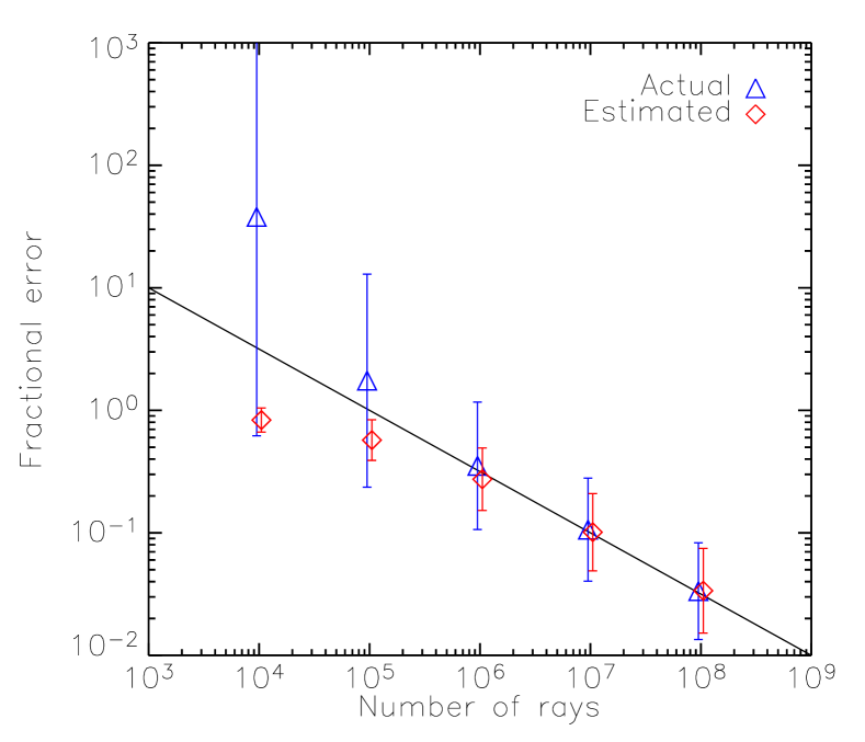
This formula for estimating the uncertainty has been tested on the pixel-by-pixel brightness in one of the cases of the clumpy scattering medium of Witt & Gordon (1996) against which the code is tested in Section 5.3. This test is shown in Figure 1. For different numbers of rays, the estimated variances in the pixel values from equation 34 were compared against the empirically determined variances from 30 runs with different random numbers. For small numbers of rays, there are many pixels which have one or no contribution, and the variance is severely underestimated. As the number of rays increases, the variances estimated using equation 34 converge toward the empirically determined values, but does so from below. This emphasizes an important fact about variance estimates using the next-event estimator: the results tend to be dominated by rare, large contributions, so unless the problem phase space has been thoroughly sampled, the true variance will be underestimated. (In fact, if scatterings can take place close to the camera, the true variance is not even finite, as previously mentioned.)

As seen above, it is necessary to save not only the quantity itself but also the sum of the squared contributions to determine the uncertainty. This increases the amount of data to keep track of by a factor of two, and makes the parallelization of the algorithm more complicated. Because of this, the uncertainty is normally not estimated in the galaxy merger simulations (The outputs from one run are already frequently larger than 1 Gb).

3.10 Clumpy Dust Distributions

Many authors have studied the effects of clumpy distributions of dust (Witt & Gordon, 1996, 2000; Bianchi et al., 2000) and reached the conclusion that it can profoundly affect the attenuation of radiation for a given mass of dust. The general tendency is for clumping to decrease attenuation and reddening by allowing radiation to escape through optically-thin lines of sight, unless the sources themselves are embedded in the clumps, in which case the attenuation can be higher than the corresponding homogenous scenario.

In sunrise, dust is assumed to be uniformly distributed within each grid cell. There is no additional clumping assumed beyond what is actually present in the adaptive grid. In our hydrodynamic galaxy merger simulations there are large-scale inhomogeneities, such as spiral structure, present, but the resolution (and the physics incorporated, for that matter) is too coarse to resolve e.g. individual molecular clouds. The adaptive grid structure could be used to put in artificial clumping on yet smaller scales, but the computational requirements would be prohibitive. One solution would be to incorporate clumping through a sub-grid analytical approximation, such as the “mega-grains approximation” (Neufeld, 1991; Hobson & Padman, 1993; Városi & Dwek, 1999); large clumps can be treated as enormous dust grains, with an effective albedo and scattering function. Clumps of dust can then be added within the existing framework as just another source of scattering. If the sources of emission are located within the clumps, however, this approach will not work. This can instead be accommodated by changing the characteristics of the emitted radiation before injecting the rays into the grid.

4 Auxiliary Calculations – Radiative Transfer in Hydrodynamic Simulations

In section 3, the core radiative-transfer algorithm of sunrise was described. However, in order to generate images and spectral energy distributions from hydrodynamic N-body simulations, the purpose for which the code was written, additional steps are necessary. These extra steps are described in this section.

The general procedure is as follows: first, hydrodynamic simulations are used to generate the geometry of the problem, e.g. merging galaxies. A number of snapshots at different time steps are saved, and for each of these a series of preparatory steps is performed. First, a stellar population synthesis model is used to calculate the SEDs of the emitting sources. Second, the adaptive grid needed for the radiative-transfer calculations is generated. Third, the radiative-transfer calculations are done. (Work is currently being done to integrate the polychromatic version of sunrise into this framework. The hydrodynamic simulations processed so far have used to the monochromatic version of sunrise.) Finally, a post-processing step is done, where the full SED is calculated by interpolating over wavelength.

4.1 The Hydrodynamic Simulations

The hydrodynamic simulations have been described in detail elsewhere (Cox, 2004; Jonsson et al., 2006; Cox et al., 2005). In particular, the specific galaxy models which are being used for the galaxy merger simulations are described in Jonsson et al. (2006) and will not be discussed here, but in order to provide a context and define the quantities used in the radiative-transfer calculations, a brief overview of the technique used will be given.

The simulations are done using GADGET (Springel et al., 2001; Springel, 2005), a Lagrangian Smooth Particle Hydrodynamics (SPH) code. The galaxies are initially modeled as a disk of stars and gas, a stellar bulge, and a dark-matter halo. The stars and dark-matter particles are collisionless and only feel the force of gravity. The gas particles are also subject to hydrodynamic forces. A collisionless particle $i$ is characterized by its mass $m_{i}$ and its gravitational softening length $r_{i}$. A gas particle has, in addition, an associated SPH smoothing length, $h_{i}$, which indicates the size of the region over which the hydrodynamic quantities associated with the particle are averaged. The smoothing length is determined by the distance to neighboring gas particles, i.e. by the gas density, such that the resolution is higher in high-density regions and lower in low-density regions where the particles represent a very smoothed-out gas density field.

During the simulation, the star-formation rate of each gas particle is calculated according to a “Schmidt law”,

$$\frac{\mathrm{d}\rho_{\star}}{\mathrm{d}t}\propto\rho_{\rm{gas}}^{1.5}\>.$$ (35)

As stars form, gas is transformed into collisionless matter. In the simulations, this is implemented in a stochastic sense (Springel & Hernquist, 2003) in which each gas particle spawns a number of stellar particles with a probability consistent with the calculated star-formation rate. These “new star” particles represent associations of single stellar populations, though their mass, typically $10^{6}\,\mathrm{M}_{\odot}$, is larger than most observed young star clusters. In addition to the quantities associated with all collisionless particles mentioned earlier, new star particles are also characterized by a formation time $t_{{\rm f},i}$ and a metallicity $Z_{i}$, which is the metallicity of the gas particle from which it is spawned.

Associated with star formation is supernova feedback, whereby energy from supernovae is deposited into the interstellar medium. This energy heats and pressurizes the gas and stabilizes it from further gravitational collapse. Including feedback is crucial for the stability of the simulations, but it is a complicated subject and many different approaches to implementing it exist. Here, it will only be mentioned that our simulations contain feedback and that a significant effort has gone into constraining this part of the simulations (Cox et al., 2005). Feedback from AGN could also affect the gas. This has been included in GADGET simulations (Springel et al., 2005), and these simulations can also be processed by sunrise.

A third consequence of star formation is chemical enrichment. Since the goal is to simulate the effects of dust, tracking metal production is naturally a topic of interest as the amount of metals available will affect the amount of dust present. In the simulations, metal production is implemented using an “instantaneous-recycling” scheme: stars formed are assumed to instantly become supernovae, and the metals produced are put back into the gas phase of the particle. Every gas particle is, in addition to the quantities mentioned earlier, characterized by a metallicity $Z_{i}$. This scheme, while simple, has several drawbacks: First, metals do not diffuse from the gas particle from which they were made, and if this particle is completely turned into stars, all the metals are incorporated into the stars and lost from the ISM. Second, while metals are recycled in supernovae, gas is not. In reality, a stellar population returns a non-negligible fraction of its mass to the gas phase, due to supernovae and stellar winds. Third, while instantaneous recycling may be a reasonable approximation for Type II supernovae, it is surely not for Type Ia supernovae which are believed to explode at least several hundred million years after the stars are formed. Improved models for metal enrichment in GADGET have been developed (Scannapieco et al., 2005), but our simulations have so far not used these.

4.2 Calculation of Stellar SEDs

After the hydro simulations have been completed, the first step is to calculate an SED for the stellar particles in each simulation snapshot. In this work, the SEDs used are from Starburst99 (Leitherer et al., 1999) but are subsampled to 510 wavelength points in order to minimize file size. (Note that this is not the much smaller number of wavelengths for which the monochromatic radiative-transfer calculations are done.) The calculation of the stellar SED is trivial since the assumption is that stellar particles represent single stellar populations, so one simply has to pick an SED with the age and metallicity of the particle.

For stars present at the start of the simulation, i.e. the disk and bulge components of the merging galaxies, the star-formation history and metallicity distribution must be specified as input parameters. Typically, the bulge stars are assumed to have formed in an instantaneous burst a relatively long time ago, while the disk has had an exponentially declining star-formation rate starting at the time of bulge formation and leading up to the start of the simulation, but any choice can be made. Formation times consistent with these assumptions are then drawn randomly for the individual particles.

The physical size of the region over which the particle luminosity is distributed is set to some fixed value. Typically, the gravitational softening length $r_{i}$ is used.

4.3 Creating the Adaptive Grid

The amount of dust is based on the amount of metals present in the galaxy simulations. As was described in section 3, the ray tracing is done on a grid, so it is necessary to transform the density field described by the particles onto a grid. In order to be able to resolve the small high-density regions in the simulations, while still covering the large volume over which the interaction takes place, this grid is adaptive (Wolf et al., 1999; Kurosawa & Hillier, 2001; Harries et al., 2004; Stamatellos & Whitworth, 2005). The grid structure is based on a regular Cartesian grid, in which grid cells can be recursively refined by subdividing them into $2^{3}$ subcells, leading to an octtree-like memory structure.

Grid construction proceeds as follows. First, the base grid is created. This grid covers the entire extent of the geometry to be simulated, and typically has $10^{3}$ grid cells. Each of these cells is then recursively subdivided until $l_{c}<\min_{i}(h_{i})c$, i.e. the cell is smaller than the sizes of all particles contained within it. This strategy uses the information contained in the SPH smoothing length to determine the smallest scale which possibly contains structure. The constant $c$ is a fudge factor, typically chosen to be 2, since this is roughly the region over which the particle contributes density. (The SPH smoothing kernel extends to $2h_{i}$.)

Once the refinement step is completed, the mass of metals contained in the particles is projected onto the grid cells using the SPH smoothing kernel as the radial density profile. For the projection, the piecewise polynomial kernel in Hernquist & Katz (1989) is used. Performing this three-dimensional integral is time-consuming, and therefore a tabulated version is used. In the cases where the particle is much larger than the grid cell, the density associated with the particle is assumed to be constant over the extent of the grid cell, eliminating the need for the integration.

At this point, the grid describes the spatial distribution in the simulations but not necessarily in the most efficient way. Unlike in, for example, an adaptive-mesh hydrodynamics code, the necessary size of the grid cells does not depend on the magnitude of the density, only on its inhomogeneity. There is no size scale that has to be resolved, as long as the problem is described accurately. (This is not true for the determination of the radiation intensity, since this can obviously change even if the dust density is perfectly uniform. Unfortunately, there is no local criterion for determining the resolution required to resolve the radiation field without actually solving the radiative-transfer problem.) Given this fact, it is desirable that cells whose quantities are sufficiently uniform be unified into one larger cell, as the ray tracing takes approximately constant time per grid cell traversed. Subcells are unified and replaced with their “parent” cell as long as the following criterion is fulfilled:

$$\left(\frac{\sigma(\rho_{\rm{met}})}{\left<\rho_{\rm{met}}\right>}<{\mbox{ tol }\!}_{\rm{met}}\right) \left(\sigma(\rho_{\rm{met}})<\frac{V_{\rm{grid}}^{-2/3}}{\kappa N}\right)\>,$$ OR (36)

where the average ($\left<...\right>$) and standard deviations ($\sigma$) are calculated over the subcells, $V_{\rm{grid}}$ is the volume of the entire grid, $N$ is the number of Monte-Carlo rays to be traced, and $\kappa$ is an opacity ($\mathrm{d}\tau/\mathrm{d}x$). Two different kinds of criteria are used: The first is a relative one; the standard deviation of the quantity over the subcells divided by the average quantity (the value the unified cell would have) must be less than a specified tolerance ($\rm{tol}_{\rm{met}}$) for unification to be allowed. This ensures that inhomogeneities are resolved. The second criterion is an absolute one; the standard deviation of the subcells must be smaller than some value. The idea is that if the difference in the quantity resulting from unification is so small that not even one Monte-Carlo ray will be affected by such a change, we can unify the cells regardless of how large the fractional deviation is. This ensures resources are not wasted on resolving regions that are so sparse they will not matter to the results anyway.

If we have $N$ rays traversing the volume $V_{\rm{grid}}$, the number traversing a subvolume $v$ will be $n=N(v/V_{\rm{grid}})^{2/3}$, if we assume a uniform and isotropic distribution of rays. The number of rays that will interact in the subvolume is

$$n_{s}\approx n\Delta\tau=n\kappa\rho\Delta\ell=\frac{N\kappa m}{V_{\rm{grid}}^{2/3}}\>,$$ (37)

interestingly independent of $v$. From this one can conclude that a deviation in mass can be accepted without affecting a single scattering if

$$\Delta m<\frac{V_{\rm{grid}}^{2/3}}{\kappa N}\>.$$ (38)

Since this result is valid for a uniform and isotropic distribution of rays, which is a questionable assumption, it is obviously not to be trusted in detail. It does however provide a scaling, and to ensure cells are not excessively unified, $N$ is usually taken to be at least $10\times$ the number of Monte-Carlo rays actually used.

The grids used for the galaxy merger simulations are constructed with $\mbox{ tol }\!_{\rm{met}}=0.1$, $N=10^{7}$ and $\kappa=3\times 10^{-5}\rm{\,{\rm kpc}}^{2}\!/\,\mathrm{M}_{\odot}$. With these parameters, the grids typically have 30k to 100k cells and cover a volume of $(200\rm{\,{\rm kpc}})^{3}$, with a maximum of 10 subdivisions. This is the equivalent resolution of a ${10240}^{3}$ uniform grid. Given the run-time scaling in Section 6.2, the use of an adaptive grid allows the simulations to complete in 2% of the time that would be required for a uniform grid. Clearly this dynamic range, which matches the dynamic range in the hydro simulations themselves, would not be possible without an adaptive grid.

It is also worth mentioning that although this description was based on building the grid from the information in the hydro simulations, the code includes a generic “grid factory” class which can be used to build the grid using density fields from any source. In addition, the grid can contain diffuse emission and the refinement also take the inhomogeneities in emissivity into account.

4.4 The Radiative-Transfer Stage

The radiative-transfer algorithm as described in detail in section 3 is repeated for a number of wavelengths in order to get an idea of the appearance of the system at all observed wavelengths, and to determine the total amount of energy absorbed by the dust. The assumption is then that since the dust properties change smoothly with wavelength, the results can be interpolated over wavelength to give a full SED.

The radiative-transfer stage is done in two phases. First, a run without considering any dust effects is done. The entire SED (all wavelengths at once) is simply propagated from randomly drawn emission sites directly to the cameras using Equation 12, giving images of the object. This is possible since without dust there is no wavelength-dependent part to this process. These “dust-free” images serve as a basis for the later interpolation over wavelength. Second, the full radiative transfer including scattering and absorption is done for a number of wavelengths from the far-UV to the near-IR. This range includes practically all the energy emitted by stars, so energy outside of this range is ignored. The number of wavelengths used is a trade-off between accuracy and computation time. For the galaxy simulations, 19 wavelengths, shown in Table 2, have been used. They were determined through a fitting procedure where the error in the fraction of the luminosity absorbed by dust was minimized against a test run using 100 wavelengths, and are particularly dense around the $2200\,{\rm\AA}$ feature in the Milky-Way dust extinction curve to ensure that this region of the spectrum is calculated accurately.

Wavelength/m	Wavelength/m (cont.)
$2.09\cdot 10^{-8}$	$3.45\cdot 10^{-7}$
$5.03\cdot 10^{-8}$	$3.94\cdot 10^{-7}$
$7.18\cdot 10^{-8}$	$4.15\cdot 10^{-7}$
$9.06\cdot 10^{-8}$	$4.86\cdot 10^{-7}$ (${\mathrm{H}\beta}$)
$1.38\cdot 10^{-7}$	$4.88\cdot 10^{-7}$
$1.56\cdot 10^{-7}$	$6.56\cdot 10^{-7}$ (${\mathrm{H}\alpha}$)
$1.83\cdot 10^{-7}$	$6.58\cdot 10^{-7}$
$2.04\cdot 10^{-7}$	$9.00\cdot 10^{-7}$
$2.39\cdot 10^{-7}$	$1.80\cdot 10^{-6}$
$2.54\cdot 10^{-7}$	$4.99\cdot 10^{-6}$
$2.67\cdot 10^{-7}$

Table 2: The wavelengths for which the radiative-transfer calculation is done.

The assumption of smoothness as a function of wavelength is not valid if one considers line emission such as ${\mathrm{H}\alpha}$. While the dust properties do not change over the line wavelength, the emission properties change abruptly; emission lines come from star-forming regions, which are generally more deeply embedded within the dust than are the sources contributing to the continuum around the line. This means that emission lines can have an attenuation many times larger than the continuum around them, and as a consequence their dust dependence must be calculated by specifically doing the radiative transfer in the line. Currently, the hydrogen lines ${\mathrm{H}\alpha}$ and ${\mathrm{H}\beta}$ are included, as these are frequently used as star-formation and dust indicators.

4.5 Post-processing

After the radiative-transfer calculation has been done, the results are interpolated to give an SED with the wavelength resolution of the stellar models. For every pixel in the output images, the attenuation, defined as the surface brightness in the image calculated including the effects of dust divided by the surface brightness in the image not including dust, is calculated for each of the radiative transfer wavelengths. This attenuation is then interpolated over all the wavelengths in the stellar-model SED, and this interpolated function is multiplied by the dust-free SED. This procedure yields an SED which has all the spectral features of the stellar model, with a large-scale behavior determined by the dust attenuation. The only exception to this is when the attenuation is $\gg 1$, i.e. there is more light in the images with dust than in those without. This frequently happens when light is scattered by dust in regions that contain no emission. In these cases, the attenuation is of questionable meaning, and the SED is interpolated directly from the radiative-transfer results. (Even in the cases where the attenuation is $<1$, the interpolated SED is an approximation since it does not account for the small-wavelength spectral features of light scattered into the line of sight, only for those present in the direct light. When sunrise is updated to use the polychromatic algorithm for the galaxy simulations, this will no longer be an issue.) These data cubes are then integrated over a number of filter passbands to generate broadband images of the simulated object.

Also during the postprocessing stage, the total luminosity absorbed in every grid cell is calculated by interpolating the absorbed luminosity at the radiative-transfer wavelengths and integrating over all wavelengths. By energy conservation this is equal to the total luminosity reradiated by the dust in the mid- and far-infrared, and images of the reradiated luminosity are then generated by assuming zero opacity and using Equation 12.

While there is no self-consistent calculation of the dust temperature distribution and hence the SED of the radiation emitted by the dust, as done by e.g. Misselt et al. (2001), a rough idea of what the infrared SED should look like, in the context of galaxies, is provided by the templates of Devriendt et al. (1999). These templates provide the dust emission SED of the galaxy as a function of its total infrared luminosity, which makes it possible to estimate the total luminosity in any given far-infrared passband. It does not provide an estimate of the spatial variations of the dust-emission SED, so constructing images of the far-infrared emission can only be done assuming all cells have the same dust-emission SED. A self-consistent calculation of dust temperature is a planned upgrade to the code.

Images are also generated for other quantities from the hydrodynamic simulations. The quantities imaged are mass density of stars, gas and metals, star-formation rate, bolometric luminosity, mass- and luminosity-weighted stellar age, and gas temperature. These images make it possible to correlate the emerging radiation and the dust effects with physical quantities of the system on a pixel-by-pixel basis.

5 Tests

With any scientific code, it is crucial to test it against independent results, either calculated analytically or using another (hopefully correct) code. The full radiative-transfer problem, with nonisotropic scattering, absorption and arbitrary geometry is far too complicated for analytic solutions, so the code has been tested against published results obtained with other Monte-Carlo codes. Sections 5.1 – 5.3 show comparisons with simpler scenarios in which the geometry is well-defined and does not factor into the uncertainty. Section 5.4 show how the polychromatic algorithm performs. Finally, in Section 5.5, sunrise is used to calculate the 2D benchmark problem from Pascucci et al. (2004), which is also used to demonstrate the relative efficiencies of the mono- and polychromatic methods.

5.1 Comparison to Witt (1977)

Figure 2: The radial brightness profiles of a nebula with an embedded star, in comparison with Witt (1977c). The plots show the surface brightness of the nebula, normalized by the flux of the star, as a function of the angular distance away from the star. The sunrise results are shown as lines, while the W77c results (after multiplying them by 2, see text) are shown as points. The four panels explore the dependence of the results on four different parameters: In the upper left, the dependence on viewing angle (W77c, Table 7); in the upper right, dependence on scattering asymmetry (W77c, Table 10); in the lower left, dependence on albedo (W77c, Table 11); and in the lower right, dependence on optical depth (W77c, Table 4). In general, the agreement is good except that sunrise seems to systematically predict a less steep rise in brightness close to the star. As explained in the text, this is consistent with the wide bins used by W77 along with the steep rise in surface brightness for small radii. There also appears to be a trend, in the upper left plot, for the sunrise results to rise faster than the W77c data towards more oblique angles. The most seriously discrepant case is the $a=1$ case in the lower left, where W77c predicts a much higher surface brightness than that predicted by sunrise. The origin of this discrepancy is unknown.

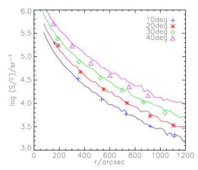
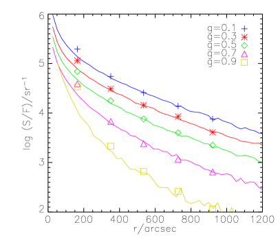
In a series of papers, Witt (1977a, b, c, hereafter collectively referred to as W77) used a Monte Carlo radiative transfer code to calculate the emerging surface-brightness distribution from a reflection nebula. This work is a suitable test for radiative-transfer calculations, because the problem geometry is simple and the papers contain an extensive study of how the surface-brightness distribution is affected by changing the input parameters. The nebula consists of a cylindrical, homogenous slab of dust. The star is located along the centerline of the cylinder, either in front of the dust, or embedded within it. The surface-brightness distribution was then described by the quantity $S/F$, where $S$ is the surface brightness of the nebula and $F$ is the flux from the star, observed at the distance of $126\mathrm{pc}$, as a function of the angular distance from the star. In sunrise, the adaptive grid was used to approximate the analytically defined cylinder used by W77. In practice, the results were insensitive to the degree of grid refinement used.

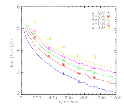
A selection of the cases calculated by W77, varying the viewing angle, grain albedo, scattering asymmetry, and optical depth of the nebula, are presented in Figure 2. In general, the results agree well, after a constant factor of 2 discrepancy in surface brightness has been accounted for. This discrepancy, in the sense that the W77 results are too low, appears attributable to a normalization error in the W77 results (A. Witt 2000, private communication), as it has been confirmed by other codes (A. Watson 2000, private communication). There is a systematic trend where sunrise  predicts a less steep rise in surface brightness close to the star, but this is consistent with the expected effect from the wide radial bins used by W77 in combination with the steep non-linear rise in surface brightness towards the center.

The largest discrepancy is the $a=1.0$ case in the lower left of Figure 2, where W77 predicts a surface brightness significantly higher than sunrise. The origin of this discrepancy is unknown, but unlike the W77 data, the sunrise results appear to be the extrapolation of the lower albedo data.

5.2 Comparison to Watson & Henney (2001)

Figure 3: Comparison with Watson & Henney (2001), showing the luminosity (or, more accurately, the radiative intensity) emerging in different directions from an infinite slab. On the left, the equivalent of their figure 1, where a point source is sitting on the surface of the slab, and on the right the equivalent of their figure 2, where a collimated beam is radiating into the surface. The WH01 results are shown as diamonds, the sunrise results as asterisks. Direct and singly scattered light is in blue (WH01 separated this into direct and singly scattered light, but that is not easy to do by default in sunrise), double-scattered light in red and triply scattered and above in green. The results agree to a remarkable degree.

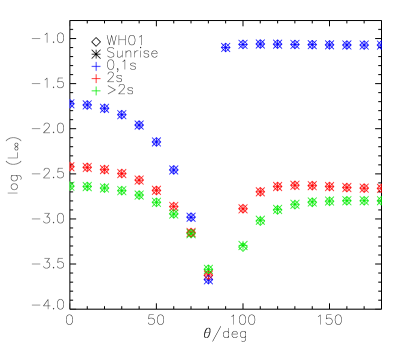
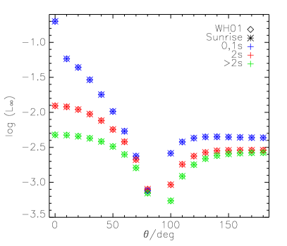
Watson & Henney (2001) presented a problem geometry very similar to the W77 study, and argued that this was a suitable test for radiative-transfer codes in that it was simple but yet nontrivial. In this problem, an infinite plane-parallel slab of unit optical depth is illuminated either by a point source on the surface of the slab or by a collimated beam incident along the normal of the slab. (While the extent of the slab is described as infinite, this violates those authors’ own definition of the set of problems they are treating, in which the opaque region is only of finite extent. This restriction applies also to sunrise, so the slab was made finite but much larger than its thickness.) In contrast with W77, Watson & Henney (2001) used the “radiative intensity” instead of the surface brightness. The radiative intensity is the total flux resulting from the source region, at large distance, multiplied by the distance squared. This quantity, which is independent of distance, can be determined even in cases where the source is unresolved. Figure 3 shows the radiative intensity in different directions using the point source and collimated beam. The results have been split into three categories: direct plus single-scattered light, doubly scattered light, and more-than-doubly scattered light. (sunrise has no explicit facilities for selecting light depending on its history, but by comparing runs with different $I_{\rm{min}}$, this can be extracted.) The sunrise results agree remarkably well with the ones presented by Watson & Henney (2001).

5.3 Comparison to Witt & Gordon (1996)

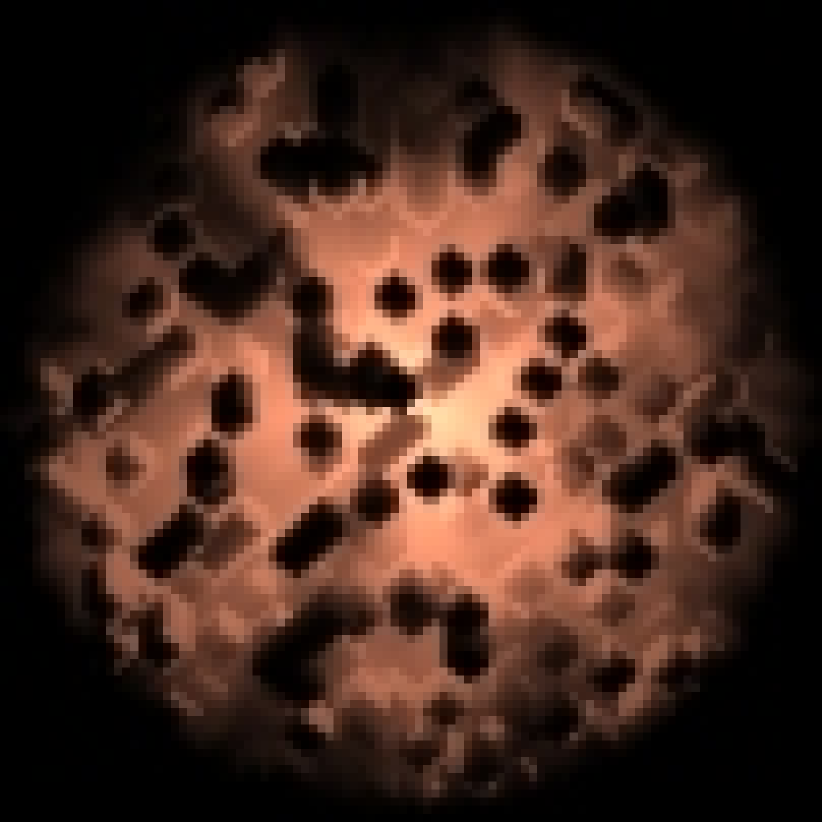
As a more complicated test, the “clumpy scattering environments” of Witt & Gordon (1996, from now on WG96), was replicated and the results compared. Briefly, WG96 investigated the escape of radiation from a clumpy environment consisting of a spherical region built up by smaller cubes of randomly assigned high- or low-density material illuminated by a central point source. The setup is described by 4 parameters: the filling factor, $f\!f$, the fraction of cells which have high density; the density contrast, $k$, the ratio of opacities between the low-density and high-density cells; the grid resolution, $N$; and the optical depth of a homogeneous distribution with the same amount of dust, $\tau_{H}$. WG96 also defined the effective optical depth $\tau_{\rm{eff}}=-\ln(L_{\rm{dir}}/L_{\rm{tot}})$, where $L_{\rm{dir}}$ is the direct luminosity escaping through the distribution, without scattering, and $L_{\rm{tot}}$ is the source luminosity. An image of a realization of these clumpy regions is shown in Figure 4.

This test is more difficult to perform conclusively, because the problem geometry itself is random. To get accurate results, not only must the emerging luminosity be averaged over sufficiently many lines of sight, but enough realizations of the clumpy medium must also be used. WG96 did not described the number of lines of sight or the number of realizations of the medium used, but our results indicate that at least 150 lines of sight and 60 realizations were necessary to obtain reasonably converged results. Even so, significant uncertainties in the sunriseresults remain. The uncertainties in the results obtained by WG96 are unknown.

Due to the nature of the grid used by sunrise, the problem cannot be compared exactly; in WG96, the ray tracing was terminated when the rays pass through a sphere inscribed within the grid, but this cannot be done in sunrise. Instead, the adaptive grid was used to approximate a spherical surface, leading to a slightly “tiled” surface, as opposed to smooth, spherical one. Four subdivisions were used, for which the results were largely converged. In any case, the uncertainty due to this effect is dwarfed by the uncertainty due to the averaging over lines of sight and realizations of the medium.

Figure 4: Image of the radiation emerging from a realization of the Witt & Gordon (1996) random clumpy medium, with parameters $\tau_{H}=10$, $f\!f=0.10$, $k=0.01$, and $N=20$. Most radiation is emerging on paths through the low-density medium. The inner surfaces of the high-density clumps can be seen as bright edges due to the efficient scattering of light off of them, while dark shadows are cast towards the outside.

Figure 5: Comparison with figures 8 – 9 of Witt & Gordon (1996): scattered luminosity emerging from the clumpy system vs. effective optical depth, for a range of density ratios ($1\geq k_{2}/k_{1}\geq 0.001$) in steps of factors of $\sqrt{10}$, starting with $k=1$ at $\tau_{\mathrm{eff}}=10$. On the left, the equivalent of figure 8 in WG96, three different filling factors, $f\!f$, are shown in different colors, while on the right, the equivalent of figure 9 in WG96, the colors indicate different grid grid resolutions, $N$. The WG96 points are connected by lines, while the corresponding sunrise points, for a number of different random realizations, are found immediately to the right and below. In general, as the density contrast departs from unity, the effective optical depth is lowered, and the scattered luminosity increases. The sunrise results agree with WG96 for the $k=1$ case, and for large $N$, but in other cases sunrise predicts systematically higher $\tau_{\mathrm{eff}}$ and lower $L_{\mathrm{scat}}$.

Figure 6: Radial surface brightness distributions of light for a range of density ratios ($1\geq k_{2}/k_{1}\geq 0.001$). This is the equivalent of figure 15 in Witt & Gordon (1996), but for clarity the different cases have been separated into two plots. The sunrise results are shown as lines, and the WG96 results as points. The sunrise results fall off more sharply towards the edge, but over a large range of radii the agreement is good. The sharp rise in the sunrise lines compared to the innermost WG96 point is because the direct light from the central point source is included in the sunrise results, but has been removed in the WG96 data.

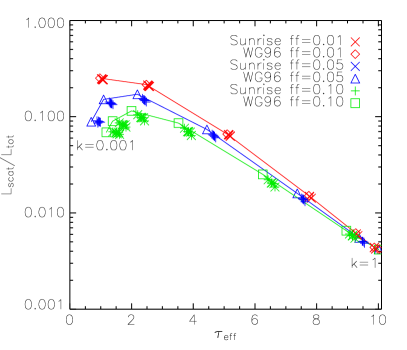
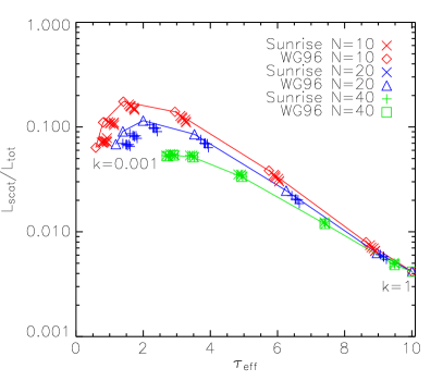
Two tests are done. The first is the equivalent of figures 8 and 9 in WG96, where the ratio of the scattered luminosity, $L_{\rm{scat}}$, the luminosity escaping the system after scattering at least once, to the total luminosity is plotted against $\tau_{\rm{eff}}$ for varying values of the density contrast $k$. The results are shown in Figure 5. As the density contrast departs from unity, the effective optical depth is lowered and the scattered luminosity increases. This is a natural consequence of clumping, as low-density paths open up through the medium and allow radiation to escape. The sunrise results agree with those of WG96 very well for the homogenous case, but as the density contrast increases, the sunrise points show systematically higher $\tau_{\rm{eff}}$ than the WG96 ones. The discrepancy seems to decrease as the number of grid cells increase; the $N=40$ case agrees within the statistical uncertainty.

The statistical spread in the sunrise points is strongly correlated. The main cause of this uncertainty is the random variation in the number of high- vs. low-density cells in the grid. Realizations in which the number of high-density cells is small will have smaller $\tau_{\rm{eff}}$ and larger $L_{\rm{scat}}$. Interestingly enough, this variation is also generally in the direction towards the WG96 results. Experiments showed that artificially lowering $f\!f$ by about 0.015 from the $f\!f=0.10$ case, while keeping the opacities unchanged, will largely remove the discrepancy between the sunrise and WG96 points. However, this does not work very well for $k\la 0.01$, and is probably not the cause of the discrepancy, the origin of which remains unknown.

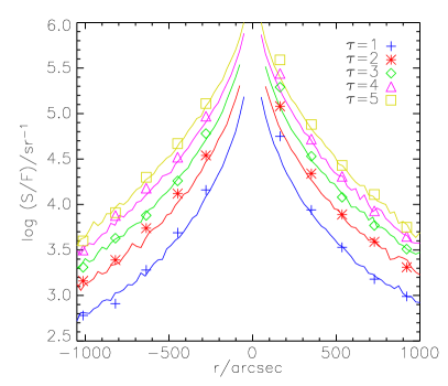
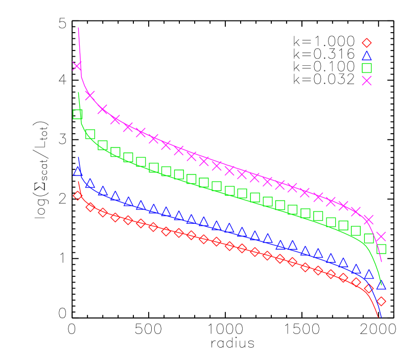
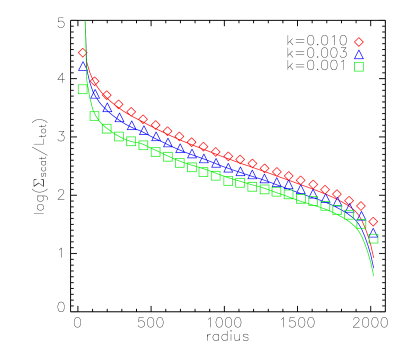
The second test is the equivalent of figure 15 in WG96. This compares the radial surface brightness distribution of scattered light, averaged over many viewing directions and realizations of the clumpy medium, for the case $\tau_{H}=10$, $f\!f=0.10$ and $N=10$. The results are shown in Figure 6. As the density contrast departs from unity, the overall surface brightness of the scattered light increases from the homogenous case, and the distribution becomes more peaked towards the center. For very small contrast ratios, when the low-density cells are already optically thin, the surface brightness again begins to decrease.

Because the WG96 figure is plotted with “arbitrary units” on the x-axis, it has been assumed that the interval plotted is the full extent of the object. The units of their surface brightness are also not specified, so the sunrise results have been adjusted so that the $k=1$ case agrees with WG96. The sunrise lines agree well with the WG96 results over a large range of radii, but fall off more quickly towards the edge. The sunrise results are also more sharply peaked compared to the innermost bin of WG96, but this is because the direct light from the point source in the center has not been removed. There is also agreement in some of the finer structure, for example a small bump in the surface brightness at $r\approx 450$ for the $k=0.001$ case, corresponding to the radius of the innermost grid cell boundary.

As seen, there are some systematic differences between the WG96 results and those determined using sunrise. However, the discrepancies are not large, and both results share the same qualitative behavior. While it would be desirable to pin down the cause of the discrepancies, we do not believe that they are severe enough to cause alarm.

5.4 Tests of the Polychromatic algorithm

Figure 7: The polychromatic algorithm tested on the W77 problems. The three plots show the deviation in surface brightness between the polychromatic results, where all 13 test cases were calculated simultaneously, and the monochromatic results presented in Figure 2. The different cases have been displaced from zero for clarity. For each test case, results using three different reference opacities and scattering asymmetries are shown by different colored lines. In general, the agreement is good. There is significantly more noise in those cases where the reference values differ greatly from the case being tested, most notably the bottom blue line in the left plot where very forward-scattering dust ($g=0.9$) is being traced with practically isotropically scattering dust ($g_{\mathrm{ref}}=0.1$). Increased noise is also evident in the top left green line ($g=0.1,\,g_{\mathrm{ref}}=0.9$) and the bottom right blue line ($\kappa=5,\,\kappa_{\mathrm{ref}}=1$).

Figure 8: Spectra from the galaxy merger simulations, exemplifying the effects of the new polychromatic algorithm. In both images, the red line shows the intrinsic emission in the pixel, neglecting radiative-transfer effects. The green line shows the old algorithm, where the spectrum is interpolated between 20 discrete wavelengths, and the blue line is the result from the polychromatic radiative transfer. The top plot shows a pixel containing an obscured H ii region, the bottom plot a pixel near an H ii region where the UV flux is dominated by scattered light. While the results agree well on the overall spectral shape, the new method gives significantly more realistic results especially for the small-scale spectral features, at a fraction of the runtime. Note in particular how the polychromatic algorithm predicts the appearance of the Ly$\,\alpha$ absorption line, the disappearance of the nebular Balmer continuum edge, and the increased attenuation of the Paschen$\,\beta$ line at $1.3\,{\mu\rm m}$ in the spectrum of the H ii region. The polychromatic calculation, including 500 wavelengths, used about 8 times the CPU time required for one monochromatic calculation. With monochromatic ray tracing, 500 separate wavelengths would have to be used to predict the same amount of detail, which would require a factor of 50 more CPU time.

The “polychromatic” algorithm has been tested with a preliminary implementation, showing that it does indeed reproduce the results obtained with the single-wavelength calculation, but it is not yet included in the production version of sunrise.

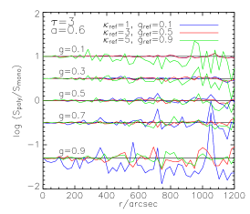
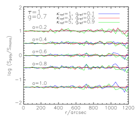
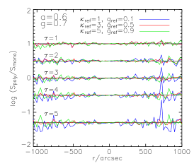
As a test, the W77 comparisons presented in Section 5.1 were redone, but now all different optical depths, albedos and scattering asymmetries were calculated simultaneously. The results are shown in Figure 7. On the whole, the agreement is excellent when the reference opacity and scattering asymmetry is close to the case being calculated. When the reference parameters are very different from the case being calculated, the results can indeed become very noisy. This is most evident in the cases where very forward-scattering dust ($g=0.9$) is being calculated using an isotropically-scattering reference case ($g_{\rm{ref}}=0.1$, or vice versa. In these cases, the weighting factor can reach values of up to 200.

Very large weighting factors can also be obtained in very optically thick cases where $\tau/\tau_{\rm{ref}}<1$. In fact, it is clear from equation 31 that in those cases $w_{\lambda}$ will increase without bound while the total contribution $w_{\lambda}exp(-\tau_{\rm{ref}})$ from those cases remains finite. This suggests that convergence will be poor, and emphasizes that a proper choice of reference parameters is crucial for the accuracy of the method; the reference wavelength should be chosen such that the range of weighting factors encountered in the problem is minimized.

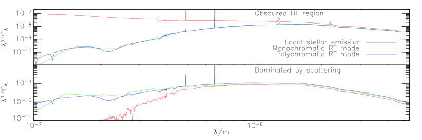
The polychromatic algorithm has also been tested on our galaxy merger simulations. This is a favorable situation, as direct light often dominates. Examples of outputs are shown in Figure 8, which shows the spectra of two different pixels in a galaxy merger simulations.

The dust opacity in a standard Milky-Way dust model varies by close to three orders of magnitude from the far-UV to the near-IR. The disadvantages of the large weighting factors resulting from this large range of opacity can be alleviated by stratifying the calculation into several ranges of wavelengths, which will restrict the range of opacities treated in the same random walk. This is used in the next section.

5.5 The Pascucci et al. (2004) 2D benchmark

Figure 9: Difference in SED between the results obtained with sunrise and the reference code radical for the Pascucci et al. (2004) benchmark problem. The monochromatic algorithm is shown in red, the polychromatic algorithm in blue. For the $\tau_{v}=100$ edge-on case, the “stratified” polychromatic calculation (see text) is shown in green. The error bars (frequently too small to be visible) indicate the $1\sigma$ Monte-Carlo sampling uncertainty in runs with $10^{6}$ rays (per wavelength for the monochromatic algorithm). The discrepancy reaches 40% for the edge-on $\tau=100$ case. The results of the polychromatic algorithm are indistinguishable from those obtained with the monochromatic one except for the most optically thick case, where the results diverge around $1\,{\mu\rm m}$. The stratified polychromatic calculation avoids this problem and agrees well with the monochromatic run. This figure is directly comparable to Figure 8 in Pascucci et al. (2004).

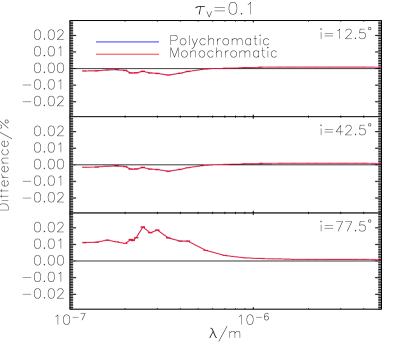
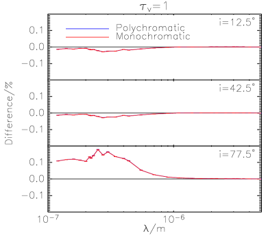
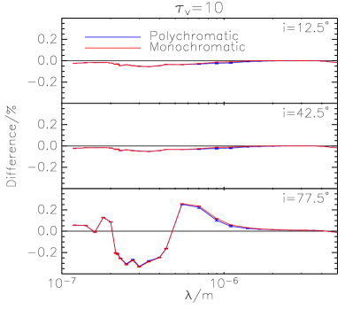
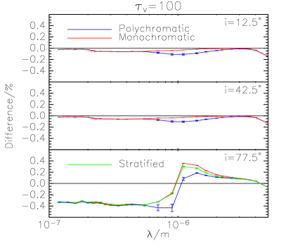
Pascucci et al. (2004, from now on P04) aimed at establishing a standard benchmark radiative-transfer problem, in the spirit of similar benchmark hydrodynamic tests, where a number of codes are compared against each other in a more complicated problem that lacks an analytical solution. They designed a two-dimensional, axisymmetric problem modeling a circumstellar disk and calculated the dust temperature distribution and emerging SED from a number of inclination angles. The optical data for the dust grains and the outputs from the 5 codes they used are available for download, which makes a detailed comparison possible. Since sunrise currently does not have the capability to calculate temperature distributions, only the SEDs at wavelengths shorter than $5\,{\mu\rm m}$, where stellar light dominates, were compared. Comparisons were done both using the monochromatic and polychromatic algorithms, which makes it possible to evaluate the efficiency of the polychromatic method in a fairly complicated problem.

The codes tested by P04 all used two-dimensional, axisymmetric grids with variable grid spacings. The orthogonal, explicitly three-dimensional adaptive-mesh grid used by sunrise is not ideally suited for such a problem, as the number of grid cells necessary to resolve the problem geometry well is much greater compared to a 2D grid. The P04 benchmark was also used by Ercolano et al. (2005) to test the MOCCASIN combined photoionization/dust radiative transfer code, which uses a (uniform) Cartesian grid.

The sunrise results are presented in Figure 9, which is analogous to Figure 8 in P04. The differences between the results using sunrise and the RADICAL (Dullemond & Turolla, 2000) code are plotted as a function of wavelength for the four different optical depths and three different inclination angles used by P04. For small optical depths the results agree very well, which is not surprising since the SED is close to the intrinsic blackbody SED of the central source. For larger optical depths, and especially for the edge-on configurations, the discrepancies reach $\pm 40\%$. This is larger than the internal differences between the codes used by P04, and is probably due to the use of an orthogonal three-dimensional grid. This hypothesis is supported by the fact that the results were converging (slowly) towards the P04 results as the grid resolution was increased. The results plotted used a grid with $1.7\times 10^{6}$ cells and a minimum cell size of $0.02\times 0.02\times 0.002\>\mbox{ AU }$. Grids with up to $4.3\times 10^{6}$ cells have been tried, and improved the agreement of around $5\%$ in the most optically thick case. The agreement between the P04 benchmark and the sunrise results is still significantly better than those presented by Ercolano et al. (2005) for the MOCCASIN code, using a uniform Cartesian grid, which disagree with the P04 results by up to a factor of 20. It is unclear what grid resolution was used by Ercolano et al. (2005).

Figure 10: The efficiencies of the polychromatic and monochromatic methods in the Pascucci et al. (2004) benchmark problem. The polychromatic algorithm is shown as solid lines, the monochromatic as dashed lines, while the color indicates the optical depth of the problem. For the $\tau_{v}=100$ case, the efficiency of the “stratified” polychromatic calculation is shown as a dot-dashed line. For lower optical depths, the efficiency of the polychromatic algorithm exceeds that of the monochromatic one for all wavelengths. For $\tau_{v}=10$, the minimum efficiency, indicating the error of the most poorly constrained wavelength, is still higher for the polychromatic algorithm. For the highest optical depth, the polychromatic calculation suffers from the large range of optical depths for different wavelengths, and shows very low efficiencies around $0.8\,{\mu\rm m}$. The stratified calculation, where wavelengths longer than $0.5\,{\mu\rm m}$ are traced separately, avoids this problem and keeps the minimum efficiency significantly higher than the monochromatic algorithm.

The benchmark was calculated using both the monochromatic and polychromatic methods. For the monochromatic calculations, $10^{6}$ rays were used for each of the 28 wavelengths used by P04 blueward of $5\,{\mu\rm m}$, while the polychromatic calculations used $10^{6}$ polychromatic rays and a reference wavelength of $0.4\,{\mu\rm m}$. Except for the $\tau_{v}=100$ case, the results are indistinguishable in Figure 9. As the optical depth increases, the polychromatic calculation becomes increasingly affected by the large range of optical depths encountered at different wavelengths. The reference wavelength used was $0.4\,{\mu\rm m}$, where both opacity and albedo are high, and as a consequence accuracy suffers at wavelengths between $0.7\,{\mu\rm m}$ and $1.5\,{\mu\rm m}$, where the opacity drops but the albedo is still fairly high. This problem was solved by “stratifying” the calculation into two wavelength ranges. The reference wavelength was kept at $0.4\,{\mu\rm m}$ for wavelengths shorter than $0.55\,{\mu\rm m}$, while longer wavelengths were traced separately, using a reference wavelength of $0.7\,{\mu\rm m}$. This two-step calculation agrees very well with the monochromatic results.

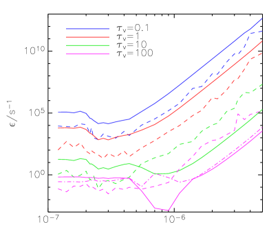
To quantify the relative efficiencies of the two methods, the “efficiency”, $\epsilon$, defined as

$$\epsilon=\frac{F_{\lambda}^{2}}{T\sigma_{F_{\lambda}}^{2}},$$ (39)

where $T$ is the CPU time required to complete the calculation and $\sigma_{F_{\lambda}}$ is the Monte Carlo sampling uncertainty in the SED, is calculated. The efficiency defined in this way is insensitive to the number of rays traced and quantifies the (inverse of the) CPU time necessary to produce results of unit relative accuracy. Figure 10 plots the efficiencies of the monochromatic and polychromatic methods as a function of wavelength for the edge-on cases in Figure 9. No effort was made to optimize the relative number of rays at different wavelengths in the monochromatic calculation.

For $\tau_{v}<10$, the efficiency of the polychromatic method exceeds that of the monochromatic one for all wavelengths. As mentioned above, the polychromatic algorithm begins to suffer at higher optical depths. For $\tau_{v}=10$, the efficiency of the monochromatic algorithm overtakes the polychromatic one at wavelengths longer than $0.5\,{\mu\rm m}$. However, the minimum efficiency, which corresponds to the wavelength with the largest error in the SED, is still higher for the polychromatic algorithm.

For the very optically thick $\tau_{v}=100$ case, the efficiency of the polychromatic algorithm plummets for the same wavelength range where the errors were large in Figure 9, reaching a minimum value much lower than the monochromatic calculation. The stratified polychromatic calculation, however, maintains an efficiency greater than the monochromatic calculation out to $1\,{\mu\rm m}$ and has a minimum efficiency significantly larger than the monochromatic results.

It is important to remember that this example used a comparably low number of 28 wavelengths. While the run time for the monochromatic method will increase linearly as the wavelength resolution is improved, the polychromatic method will scale much better (at least until the run time becomes dominated by the vector calculations as opposed to the ray tracing). It is clear that the particular strength of the polychromatic algorithm is in processing densely sampled wavelengths, not in covering a large range in wavelength.

6 Code Implementation Details

sunrise is written in C++, with a highly modular code structure. It is easy to add new types of emission, sources of scattering, etc., as these are isolated from the core radiative-transfer engine. Efficient vector calculations are provided by the Blitz++ library (Veldhuizen, 1998).

sunrise uses the implementation of the Mersenne Twister MT19937 random-number algorithm (Matsumoto & Nishimura, 1998) provided by the Blitz++ library (Veldhuizen, 1998).

6.1 Grid Traversal

Figure 11: The memory access pattern in a test run of sunrise. The graph shows the cumulative distribution of strides (differences in memory address) when accessing consecutive grid cells during a run consisting of about $10^{5}$ grid-cell-to-grid-cell steps. The minimum stride is 48 bytes, the size of the grid-cell data structure, and this is the source of the discretization of the small strides. The vertical lines indicate 4096 and 16384 bytes, the size of the TLB entries on the POWER3/Opteron and Altix 300 processors, respectively. The Hilbert ordering results in noticeably smaller strides than the default depth-first ordering, but not enough to outweigh its increased complexity.

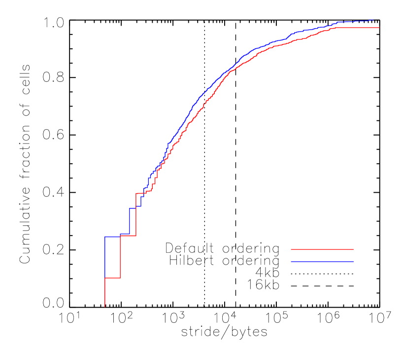
The most time-consuming part of the calculation is the grid traversal, walking the ray from grid cell to grid cell. Because the rays can traverse the grid in any direction, the memory access pattern of the code is hard to predict, and often not optimal. To minimize CPU cache and TLB (Translation Lookaside Buffer) misses, it is important to access memory in as localized a fashion as possible. This is easy in applications like matrix multiplications, where it is up to the programmer to decide in which order to access memory, but hard in the application considered here. The solution is to order the grid cells in memory in such a way that locality is preserved; grid cells that are close in space should also be stored close in memory. Since this is a mapping from 3D to 1D, it cannot be accomplished perfectly, and various approaches exist. The strategy used by sunrise is to simply store the subgrids consecutively in memory in the order they are encountered when traversing the tree of refined cells in a depth-first fashion. This actually results in a fairly compact memory access pattern. To explore the potential for improvements, storing the grid cells according to a Hilbert curve was also tried, using the algorithm described in Bartholdi & Goldsman (2001). The Hilbert curve is an example of what is known as “space-filling curves”, a one-dimensional curve which fills three-dimensional space, and has been argued as being nearly optimal for these problems (Niedermeier & Sanders, 1996). The result of this comparison is shown in Figure 11. While the Hilbert ordering did have a more compact access pattern, the differences were comparatively small and did not outweigh the accompanied increased complexity. Thus, the default memory ordering was retained.

In addition, finding neighboring cells in the grid is quite expensive, as the tree has to be traversed up the hierarchy and then down again, accessing many higher-level grid cells in the process. Because of this, sunrise utilizes a caching scheme whereby each cell saves pointers to its neighboring cells once they have been determined. This speeds up subsequent neighbor searches considerably.

6.2 Runtime Requirements

The most obvious scaling is that the runtime of the ray tracing (excluding initialization, I/O, etc.) obviously scales linearly with the number of rays traced. The time required per ray is affected by many factors, including the problem geometry, the importance of scattering, and the terminating intensity $I_{\rm{min}}$. The time is dominated by the tracing of the ray from one grid cell to the other, which takes approximately constant time. Emission and interaction events are much more rare and do not constitute the dominant computational load. From this it would be expected that the time required to trace one ray would scale with the number of grid cells, which is the case. The scaling is roughly $t_{r}\sim N_{c}^{1/3}$, which would also be the naive expectation since this is how the number of grid cells traversed by a ray should scale with the total number of cells.

Furthermore, increasing the number of cameras increases the computational load, since part of the ray propagation consists of calculating $\tau^{\rm{obs}}$, which means traversing the cells from the point of emission or interaction to each of the observers. The time taken to complete one Monte-Carlo ray can thus be split into two components such that $t_{r}=t_{0}+N_{c}t_{c}$, where $t_{0}$ is the time taken to complete the ray tracing in the absence of observers, and $t_{c}$ the time taken to traced the optical depth to an observer. This relation is indeed obeyed by the code, and the two components $t_{0}$ and $t_{c}$ are such that, in typical cases of simulated galaxies, the time proportional to $N_{c}$ becomes dominant for $N_{c}\ga 3$.

6.3 Parallelization

Any high-performance numerical code relies on parallel execution to reach high performance, so this capability was a basic requirement for the development of sunrise. The Monte-Carlo method is easy to parallelize; as long as the entire grid fits in memory, each ray is independent of others. sunrise uses multithreaded (shared-memory) parallelism during the grid creation and ray-tracing stages. As every ray is independent, communication requirements are minimal resulting in essentially perfect scaling as long as the memory bus is not saturated.

Completing the full calculation for one simulation snapshot takes 6-12 CPU hours on a contemporary dual-CPU 2.2GHz Opteron system, for typical conditions of 11 camera positions, 21 wavelengths and $10^{6}$ rays per wavelength. The total amount of CPU time consumed by the radiative-transfer calculations is roughly equal to the time used by the hydrodynamic galaxy merger simulations.

On the NASA Altix 3000 system Columbia, a cluster of machines each consisting of 256 two-processor nodes, where the full, system-wide memory is visible as a single address space using high-speed interconnects, sunrise can be used on up to 16 processors with a penalty of only 23 percent compared to running on one node.

Adding the ability to run using distributed memory would vastly increase the size of the problems that could be treated. However, it would also make the parallelization much more complicated, and as the current ability is sufficient for our computational needs, such an upgrade is not currently planned.

6.4 Distribution

As a service to the community, sunrise is available under the terms of the GNU General Public License (Free Software Foundation, 1991). Other users are encouraged to use sunrise for their radiative-transfer applications, and to add enhancements that increase its capabilities.

7 Future Improvements

There are numerous improvements that can be made to the radiative-transfer code. The polychromatic algorithm is currently being implemented in the production version of sunrise, and schemes for minimizing the impact of large weighting factors will be explored. One possibility is to split rays with large weights and scatter them in different directions (Dupree & Fraley, 2002), which will increase the sampling in the heavily weighted part of phase space. Such a scheme could be combined with “Russian roulette” into a scheme where the code attempts to keep the weights of all rays within some specified range.

The biasing of path lengths done in the polychromatic algorithm opens up other possibilities; it is well known that the Monte Carlo method has problems treating very large optical depths, for example in the case of a cloud heated by external radiation studied by Juvela (2005), because few rays make it into the opaque regions. Juvela (2005) explored the effects of biasing the distributions of the external photons and the scattering direction. Another possibility would be to bias the path lengths between scatterings to larger values, which would allow better sampling of the rare photons which penetrates unusually deep into the cloud.

These possibilities suggest that it would be advantageous to make it possible to not only use arbitrary scattering phase functions or emission distributions in sunrise, but also to provide an infrastructure for customized “biasing plug-ins” which can be selected by the user depending on the problem at hand.

Another obvious improvement is to include a self-consistent calculation of the dust emission, so predictions of infrared observations of galaxies with e.g. the Spitzer Space Telescope can be made. These calculations can be done to varying degrees of sophistication, from calculating equilibrium temperatures of single grain species to full stochastic temperature distributions of very small grains and PAH emission, but it becomes necessary to include the heating of dust grains due to the emission from other grains. This introduces a coupling between the local emissivity and radiation intensity, which makes it necessary to integrate until the dust temperature distribution converges.

An interesting alternative, applicable in situations where the opacity is not a function of temperature, is the method of Bjorkman & Wood (2001). In this method, the dust temperatures are updated whenever an absorption event happens and the energy is reemitted with an SED equal to the difference between the current emission SED and the one before the absorption event happened. This ensures that the net radiation emitted by the dust is appropriate for the temperature of the dust grains, and as more rays are traced the dust temperature distribution will relax toward the equilibrium value without iteration. Baes et al. (2005) studied this method and concluded that while it produces the correct frequency distribution in the case of grains in thermal equilibrium, the method will not work for stochastically heated grains because the probability distribution required for the reemitted radiation will become negative. As negative probabilities are unphysical, the method will fail. The polychromatic algorithm suggests a way around this obstacle: There is no obvious reason why the weights of the rays in the polychromatic algorithm can’t be negative. The problem is not fundamentally that negative probabilities are necessary, but that the grain has emitted too much energy in a certain part of the spectrum and this must be corrected for. This can be accomplished with negative weights for certain wavelengths. Since it will only serve to remove energy which was previously emitted, the radiation field should still converge towards the true value, only it will not converge from below as in the original Bjorkman & Wood (2001) formulation. This possibility will be explored in sunrise in the future.

Another important improvement for correctly predicting the SED of galaxies is a more detailed modeling of star-forming regions, which are not resolved in our galaxy simulations. Studies have shown that extra attenuation of young stellar populations are necessary for fitting dust attenuations in galaxies (Silva et al., 1998; Charlot & Fall, 2000; Tuffs et al., 2004). While the adaptive grid could be used to resolve these regions, the computational cost would be prohibitive. A better way would be to use sub-resolution models of the emission from star-forming regions (e.g. Groves et al., 2004) and feed this emission into the sunrise grid.

8 Conclusion

This paper has described sunrise, a new Monte-Carlo code for calculating the radiative transfer of light through a scattering and absorbing medium. sunrise builds on previous advanced Monte-Carlo codes (Kurosawa et al., 2004; Baes et al., 2003; Gordon et al., 2001; Bianchi et al., 2000; Lucy, 1999; Wolf et al., 1999), and adds a polychromatic algorithm, where all wavelengths are traced simultaneously, and efficient parallel computation in a flexible, modular package, making calculations with a spatial dynamical range of more than $10^{4}$ feasible. Images at any wavelength from far-UV to near-IR from an arbitrary number of directions are generated, as well as the radiation intensity and dust luminosity as a function of position in the object. In addition, sunrise  includes a framework for calculating the effects of dust in hydrodynamic simulations, and the code is freely available to the community.

Accurate radiative-transfer calculations with realistic geometries are crucial in tying theory to observations in any situation where dust significantly affects the radiation emerging from an object. This applies to such diverse a family of objects as galaxies, star-forming regions, AGN, and protostellar disks. The outputs from the radiative-transfer calculations generate “simulated observations” of the object, so comparisons with observations can be done using observational instead of theoretical quantities. This approach requires specifying many free parameters, but in reality only serves to make this dependence explicit, since if the comparisons are done with theoretical quantities, the same parameters normally need to be specified to convert observed quantities to intrinsic ones. In many cases, such as the complicated radiative-transfer situations that can be solved by sunrise, it is not even possible to invert the observations, and making observational predictions from a theoretical model is then the only avenue possible. Another advantage of comparing observational quantities is that it is usually easier to mimic selection biases and instrumental effects in simulations than to infer their effects on theoretical quantities.

sunrise is currently being used to investigate dust attenuation in simulations of isolated spiral galaxies (Rocha Gaso et al., in preparation), to generate a library of images of simulated galaxy mergers which can be directly compared to Hubble Space Telescope observations, and to quantify the timescales over which mergers result in disturbed morphologies.

The author wishes to thank T. J. Cox and Joel Primack for their help with the infrastructure to process the galaxy merger simulations, and them as well as Sandy Faber, Greg Novak, Mike Kuhlen and Brent Groves for stimulating discussions about the radiative transfer problem. Thanks also go to A. Witt and A. Watson for their assistance in pinning down the discrepancy with the W77 results, to the referee, J. Yates, for comments which improved the paper, and to I. Pascucci for help in setting up the P04 benchmark. The author is also grateful for the hospitality of the Max-Planck Institute for Astrophysics in Garching, where part of this paper was written, and for support from a UC/LLNL cooperative grant from IGPP to Wil van Breugel. This work was supported by program number HST-AR-10678.01-A, provided by NASA through a grant from the Space Telescope Science Institute, which is operated by the Association of Universities for Research in Astronomy, Incorporated, under NASA contract NAS5-26555. This research used computational resources of the National Energy Research Scientific Computing Center (NERSC), which is supported by the Office of Science of the U.S. Department of Energy, and the NASA Advanced Supercomputing Division (NAS).

References

- Baes et al. (2003) Baes M., Davies J. I., Dejonghe H., Sabatini S., Roberts S., Evans R., Linder S. M., Smith R. M., de Blok W. J. G., 2003, MNRAS, 343, 1081
- Baes et al. (2005) Baes M., Dejonghe H., Davies J. I., 2005, in AIP Conf. Proc. 761: The Spectral Energy Distributions of Gas-Rich Galaxies: Confronting Models with Data Efficient radiative transfer modelling with SKIRT. pp 27–
- Baes et al. (2005) Baes M., Stamatellos D., Davies J. I., Whitworth A. P., Sabatini S., Roberts S., Linder S. M., Evans R., 2005, New Astronomy, 10, 523
- Bartholdi & Goldsman (2001) Bartholdi J. J. I., Goldsman P., 2001, Softw., Pract. Exper., 31, 395
- Bekki & Shioya (2000a) Bekki K., Shioya Y., 2000a, ApJ, 542, 201
- Bekki & Shioya (2000b) Bekki K., Shioya Y., 2000b, A&A, 362, 97
- Bianchi et al. (2000) Bianchi S., Ferrara A., Davies J. I., Alton P. B., 2000, MNRAS, 311, 601
- Bjorkman & Wood (2001) Bjorkman J. E., Wood K., 2001, ApJ, 554, 615
- Cashwell & Everett (1959) Cashwell E. D., Everett C. J., 1959, A Practical Manual on the Monte Carlo Method for Random Walk Problems. Pergamon, New York
- Cattaneo et al. (2005) Cattaneo A., Combes F., Colombi S., Bertin E., Melchior A.-L., 2005, MNRAS, 359, 1237
- Charlot & Fall (2000) Charlot S., Fall S. M., 2000, ApJ, 539, 718
- Cox (2004) Cox T. J., 2004, PhD thesis, University of California, Santa Cruz, http://physics.ucsc.edu/~tj/work/thesis
- Cox et al. (2005) Cox T. J., Jonsson P., Primack J., Somerville R. S., 2005, MNRAS, submitted (astro-ph/0503201)
- Devriendt et al. (1999) Devriendt J. E. G., Guiderdoni B., Sadat R., 1999, A&A, 350, 381
- Draine (2003) Draine B. T., 2003, ApJ, 598, 1017
- Dullemond & Turolla (2000) Dullemond C. P., Turolla R., 2000, A&A, 360, 1187
- Dupree & Fraley (2002) Dupree S. A., Fraley S. K., 2002, A Monte-Carlo Primer. Kluwer Academic / Plenum Publishers
- Ercolano et al. (2005) Ercolano B., Barlow M. J., Storey P. J., 2005, MNRAS, 362, 1038
- Fischer et al. (1994) Fischer O., Henning T., Yorke H. W., 1994, A&A, 284, 187
- Folini et al. (2003) Folini D., Walder R., Psarros M., Desboeufs A., 2003, in ASP Conf. Ser. 288: Stellar Atmosphere Modeling A New Method for 3D Radiative Transfer with Adaptive Grids. p. 433
- Free Software Foundation (1991) Free Software Foundation 1991, GNU General Public License, http://www.gnu.org/licenses/gpl.html
- Gordon et al. (2001) Gordon K. D., Misselt K. A., Witt A. N., Clayton G. C., 2001, ApJ, 551, 269
- Groves et al. (2004) Groves B. A., Dopita M. A., Sutherland R. S., 2004, ApJS, 153, 9
- Guhathakurta & Draine (1989) Guhathakurta P., Draine B. T., 1989, ApJ, 345, 230
- Harries et al. (2004) Harries T. J., Monnier J. D., Symington N. H., Kurosawa R., 2004, MNRAS, 350, 565
- Henyey & Greenstein (1941) Henyey L. C., Greenstein J. L., 1941, ApJ, 93, 70
- Hernquist & Katz (1989) Hernquist L., Katz N., 1989, ApJS, 70, 419
- Hobson & Padman (1993) Hobson M. P., Padman R., 1993, MNRAS, 264, 161
- Jonsson (2004) Jonsson P., 2004, PhD thesis, University of California, Santa Cruz, http://sunrise.familjenjonsson.org/thesis
- Jonsson et al. (2006) Jonsson P., Cox T. J., Primack J. R., Somerville R. S., 2006, ApJ, 637, 255
- Juvela (2005) Juvela M., 2005, A&A, 440, 531
- Kurosawa et al. (2004) Kurosawa R., Harries T. J., Bate M. R., Symington N. H., 2004, MNRAS, 351, 1134
- Kurosawa & Hillier (2001) Kurosawa R., Hillier D. J., 2001, A&A, 379, 336
- Leitherer et al. (1999) Leitherer C., Schaerer D., Goldader J. D., Delgado R. M. G., Robert C., Kune D. F., de Mello D. F., Devost D., Heckman T. M., 1999, ApJS, 123, 3
- Lucy (1999) Lucy L. B., 1999, A&A, 344, 282
- Lux & Koblinger (1991) Lux I., Koblinger L., 1991, Monte Carlo particle transport methods: neutron & photon calculations. CRC Press
- Matsumoto & Nishimura (1998) Matsumoto M., Nishimura T., 1998, ACM Transactions on Modeling and Computer Simulation, 8, 3
- Misselt et al. (2001) Misselt K. A., Gordon K. D., Clayton G. C., Wolff M. J., 2001, ApJ, 551, 277
- Neufeld (1991) Neufeld D. A., 1991, ApJ, 370, L85
- Niccolini et al. (2003) Niccolini G., Woitke P., Lopez B., 2003, A&A, 399, 703
- Niedermeier & Sanders (1996) Niedermeier R., Sanders P., 1996, Technical report, On the Manhattan-distance between points on space-filling mesh-indexings. Universität Karlsruhe, Fakultät für Informatik
- Pascucci et al. (2004) Pascucci I., Wolf S., Steinacker J., Dullemond C. P., Henning T., Niccolini G., Woitke P., Lopez B., 2004, A&A, 417, 793
- Scannapieco et al. (2005) Scannapieco C., Tissera P. B., White S. D. M., Springel V., 2005, MNRAS, 364, 552
- Silva et al. (1998) Silva L., Granato G. L., Bressan A., Danese L., 1998, ApJ, 509, 103
- Springel (2005) Springel V., 2005, MNRAS, 364, 1105
- Springel et al. (2005) Springel V., Di Matteo T., Hernquist L., 2005, MNRAS, 361, 776
- Springel & Hernquist (2003) Springel V., Hernquist L., 2003, MNRAS, 339, 289
- Springel et al. (2001) Springel V., Yoshida N., White S. D. M., 2001, New Astronomy, 6, 79
- Stamatellos & Whitworth (2005) Stamatellos D., Whitworth A. P., 2005, A&A, 439, 153
- Steinacker et al. (2003) Steinacker J., Henning T., Bacmann A., Semenov D., 2003, A&A, 401, 405
- Tuffs et al. (2004) Tuffs R. J., Popescu C. C., Völk H. J., Kylafis N. D., Dopita M. A., 2004, A&A, 419, 821
- Városi & Dwek (1999) Városi F., Dwek E., 1999, ApJ, 523, 265
- Veldhuizen (1998) Veldhuizen T. L., 1998, in Proceedings of the 2nd International Scientific Computing in Object Oriented Parallel Environments (ISCOPE’98) Arrays in Blitz++
- Watson & Henney (2001) Watson A. M., Henney W. J., 2001, Revista Mexicana de Astronomia y Astrofisica, 37, 221
- Witt (1977a) Witt A. N., 1977a, ApJS, 35, 1
- Witt (1977b) Witt A. N., 1977b, ApJS, 35, 7
- Witt (1977c) Witt A. N., 1977c, ApJS, 35, 21
- Witt & Gordon (1996) Witt A. N., Gordon K. D., 1996, ApJ, 463, 681
- Witt & Gordon (2000) Witt A. N., Gordon K. D., 2000, ApJ, 528, 799
- Wolf et al. (1999) Wolf S., Henning T., Stecklum B., 1999, A&A, 349, 839
- Yusef-Zadeh et al. (1984) Yusef-Zadeh F., Morris M., White R. L., 1984, ApJ, 278, 186