X-ray and Sunyaev-Zel’dovich Effect Measurements
of the Gas Mass Fraction in Galaxy Clusters
Abstract
We present gas mass fractions of 38 massive galaxy clusters spanning redshifts from 0.14 to 0.89, derived from Chandra X-ray data and OVRO/BIMA interferometric Sunyaev-Zel’dovich Effect (SZE) measurements. We use three models for the gas distribution: (1) an isothermal -model fit jointly to the X-ray data at radii beyond 100 kpc and to all of the SZE data, (2) a non-isothermal double -model fit jointly to all of the X-ray and SZE data, and (3) an isothermal -model fit only to the SZE spatial data. We show that the simple isothermal model well characterizes the intracluster medium (ICM) outside of the cluster core, and provides consistently good fits to clusters spanning a wide range of morphological properties. The X-ray and SZE determinations of mean gas mass fractions for the 100 kpc-cut isothermal -model are (X-ray) and (SZE), where uncertainties are statistical followed by systematic at 68% confidence. For the non-isothermal double -model, (X-ray) and (SZE). For the SZE-only model, (SZE). The agreement in the results shows that the core can be satisfactorily accounted for by either excluding the core in fits to the X-ray data (the 100 kpc-cut model) or modeling the intracluster gas with a non-isothermal double- model. We find that the SZE is largely insensitive to structure in the core. Our results indicate that the ratio of the gas mass fraction within to the cosmic baryon fraction, , is where the range includes statistical and systematic uncertainties at 68% confidence. Finally, by assuming that cluster gas mass fractions are independent of redshift, we find that the results are in agreement with standard CDM cosmology and are inconsistent with a flat matter dominated () universe.
1 Introduction
Massive galaxy clusters () are thought to be the relatively recent descendants of rare high density fluctuations in the primordial universe. The evolution of massive clusters is critically dependent on cosmology, in particular on the matter density and the normalization of the power spectrum . Furthermore, as massive galaxy clusters have collapsed from volumes of order 1000 Mpc3, their composition should reflect that of the non-relativistic components of the universe, i.e., the baryon budget of a cluster should reflect .
For these reasons there is considerable interest in using cluster observations to constrain cosmology, and there has been significant success. For example, early X-ray observations were used to constrain the gas mass fraction of clusters and thereby set a lower limit to /. Using constraints on from Big Bang Nucleosynthesis, this led to upper limits on that strongly ruled out a flat matter dominated universe (White et al., 1993); a precise measurement of was not possible due to insufficient understanding of the cluster baryon budget. A low was also indicated by the discovery of high redshift () massive clusters, which should be extremely rare in a matter dominated, flat universe (Bahcall & Fan, 1998; Donahue et al., 1998).
Cosmological constraints can be obtained by exploiting the expected redshift independence of cluster gas mass fractions; only if the correct cosmology is used in the derivation of the gas mass fractions for a sample of clusters spanning a reasonable redshift range would the resulting gas mass fractions be constant with redshift (Sasaki, 1996; Pen, 1997). This technique is independent of the uncertainty in the cluster baryon budget as well as the value of the Hubble constant.
Subsequently there have been many more cosmological studies using cluster X-ray and Sunyaev-Zel’dovich Effect (SZE) measurements (e.g., see White et al., 1993; David et al., 1995; Evrard, 1997; Myers et al., 1997; Mohr et al., 1999; Ettori & Fabian, 1999; Grego et al., 2001; Allen et al., 2002; Sanderson & Ponman, 2003; Allen et al., 2004). In general the results are in good agreement, along with cosmic microwave background (CMB) (i.e., Spergel et al., 2006) and Type Ia supernova measurements (Perlmutter et al., 1999; Riess et al., 1998), with the now standard CDM cosmology.
Future large scale cluster surveys are being pursued which exploit the critical cosmological dependence of the evolution of cluster abundance to provide independent, precise determinations of , , and the equation of state of dark energy, (e.g., Kneissl et al., 2001; Romer et al., 2001; Kosowsky, 2003; Ruhl et al., 2004). The ability to extract cosmology from large surveys using SZE, X-ray, or any other cluster observable, will depend on the ability to link the measurements to cluster mass. An improved understanding of cluster structure and evolution is of interest in itself and would clearly also be helpful for improving cosmological measurements with clusters.
In this paper we investigate the gas mass fractions for a sample of 38 clusters spanning redshifts from 0.14 to 0.89, using Chandra X-ray data and BIMA/OVRO interferometric radio SZE data. This SZE cluster sample is the largest yet compiled by over a factor of two. Combining the SZE data with the high resolution Chandra X-ray data we are able to compare the SZE and X-ray gas mass fractions using two different models for the ICM. Comparison of the SZE and X-ray results allows us to place constraints on the possible systematic effects associated with our incomplete knowledge of cluster properties. The results also provide constraints on the cluster baryon budget, and thereby provide an important observational benchmark for cluster simulations. The baryon budget is sensitive to the details of cluster formation, gas cooling and star formation history of the ICM (Ettori et al., 2006). Lastly, we consider the cosmological constraints derived by assuming the cluster gas mass fractions of our sample do not evolve with redshift.
The paper is organized as follows: we review the theory underlying the X-ray emission and the SZE in clusters in §2 and describe the X-ray and SZE data in §3. In §4 we describe the cluster models and analysis methods used to determine the gas mass fractions, and we present tests of these models. In §5 we discuss additional sources of uncertainty in the gas mass fraction measurements, both statistical and systematic. The results are presented in §6, and constraints on the cluster baryon budget and cosmological parameters are detailed in §7. Finally, we summarize our conclusions in §8. All uncertainties are at the 68.3% confidence level, and a CDM cosmology with =0.3, =0.7, =0.7 is assumed unless otherwise stated.
2 X-ray emission and Sunyaev Zel’dovich Effect
X-ray emission in clusters arises predominantly from thermal bremsstrahlung for gas electron temperatures keV. The X-ray emissivity is not a directly observable quantity; instead X-ray proportional counters and CCDs measure the X-ray surface brightness over some frequency band (e.g., Sarazin, 1988),
| (1) |
where the integral is along the line of sight and is called the X-ray cooling function and is proportional to . The observed X-ray emission can also be used to measure the gas temperature using instruments with spectral capability.
The thermal SZE is a small ( mK) distortion in the CMB spectrum caused by inverse Compton scattering of the CMB photons off of energetic electrons in the hot intracluster gas (Sunyaev & Zel’dovich, 1970, 1972). The spectral distortion can be expressed for dimensionless frequency as a temperature change relative to the CMB temperature :
| (2) |
where is the Compton- parameter, is the Thomson scattering cross-section of the electron, contains the frequency dependence of the SZE, and the integral is along the line of sight. The frequency dependence can be expressed as
| (3) |
where is a relativistic correction. We adopt the analytic corrections of Itoh et al. (1998) which are good to fifth order in . The linear density and temperature dependences of the SZE make it a complementary probe to the X-ray emission, which varies as . The SZE is a decrement at low frequencies ( GHz) and an increment at high frequencies due to the up-scattering of photons by the hot electrons. There is also a kinetic SZE that arises from scattering of CMB photons in a cluster with line of sight motion relative to the CMB rest frame. Discussion of the SZE in this work refers to the thermal SZE unless otherwise specified. We address the possible effects of the kinetic SZE on our results in §5.
With knowledge of the gas temperature, one can use either or to determine the gas distribution and obtain . The total mass can be determined by assuming that the gas is in hydrostatic equilibrium (HSE) with the cluster potential. The gas mass fraction is then /.
3 Data
The cluster sample consists of clusters that have both X-ray data from the Chandra X-ray Observatory and SZE data from the BIMA/OVRO SZE imaging project, which uses the Berkeley-Illinois-Maryland Association (BIMA) and Owens Valley Radio Observatory (OVRO) interferometers to image the SZE. The BIMA/OVRO SZE imaging project has generally pursued hot clusters (published keV) which by inference should be massive and have a strong SZE. Properties of the cluster sample, including full cluster names, redshifts, positions, and Chandra and BIMA/OVRO observing information, are listed in Table 1.
The X-ray data were reduced using the Chandra Interactive Analysis of Observations (CIAO) 3.2 software package with CALDB 3.1. Details of the data reduction procedure are given in Bonamente et al. (2004) and Bonamente et al. (2006); briefly, CIAO and the CALDB are used to apply corrections for charge transfer inefficiency (CTI) and buildup of a contaminant on the optical blocking filter. The observations are filtered to contain only photons with energies between 0.7 and 7.0 keV, and to remove contamination from solar flares. The data are then binned into images for each chip relevant to the observation, and X-ray backgrounds are extracted from appropriate cluster-free regions of the chips (Bonamente et al., 2004). Exposure maps are also created with CIAO, and all spatial analysis is performed on the binned images and exposure maps. Cluster spectra are extracted from a circular region centered on the cluster containing roughly 95% of the cluster counts, again restricted to the energy range 0.7—7.0 keV. Spectra are grouped so that Gaussian statistics can be used in the spectral fitting, and a background spectrum is also extracted using the same background regions used in the image analysis. The software package XSPEC (Arnaud, 1996) is used to fit a model to the spectrum and determine the X-ray spectroscopic temperature and metallicity of the cluster.
Interferometric radio observations of the cluster SZE were performed at the Berkeley-Illinois-Maryland Association observatory (BIMA) and at the Owens Valley Radio Observatory (OVRO). The millimeter-wave arrays were equipped with 26-36 GHz receivers for the SZE observations (Carlstrom et al., 1996). Most of the OVRO and BIMA telescopes were placed in a compact configuration to provide sensitivity on angular scales subtended by distant clusters (typically ) and a few telescopes were placed at longer baselines for simultaneous point source imaging (Reese et al., 2002).
The SZE data consist of the position in the Fourier domain (- plane) and the visibilities — the real and imaginary Fourier component pairs as functions of and , which are the Fourier conjugate variables to right ascension and declination. The effective resolution of the interferometer, the synthesized beam, depends on the - coverage and is therefore a function of the array configuration and source position. A typical size for the synthesized beam for the short baseline data is . Details of the SZE data reduction can be found in Grego et al. (2001) and Reese et al. (2002). Briefly, the SZE data were reduced using the MIRIAD (Sault et al., 1995) and MMA (Scoville et al., 1993) software packages. Absolute flux calibration was performed using Mars observations adopting the brightness temperature from the Rudy (1987) Mars model. The gain was monitored with observations of bright radio point sources, and remained stable at the 1% level over a period of months. Data were excised when one telescope was shadowed by another, when cluster observations were not bracketed by two phase calibrators, when there were anomalous changes in the instrumental response between calibrator observations, or when there was spurious correlation.
Images were made with the DIFMAP software package (Pearson et al., 1994) to inspect the data quality and, using only long baseline data, to identify and fix the positions of radio point sources. The point source fluxes are included as free parameters in the model fitting, using the same methodology as Reese et al. (2002).
4 Analysis Methods and Modeling
4.1 Cluster Density Models
The isothermal -model has frequently been used in the analysis of X-ray and SZE cluster images (Cavaliere & Fusco-Femiano, 1976, 1978; Jones & Forman, 1984; Elbaz et al., 1995; Grego et al., 2001; Reese et al., 2002; Ettori et al., 2004). The 3-dimensional electron number density is given by
| (4) |
where is the electron number density, is the radius from the center of the cluster, is the core radius of the intracluster medium (ICM), and is a power law index. A convenient feature of the isothermal -model is that the X-ray surface brightness and SZE decrement profiles take simple analytic forms
| (5) | |||||
| (6) |
where is the central X-ray surface brightness, is the central thermodynamic SZE temperature decrement/increment, and is the angular core radius of the cluster.
However, recent deep X-ray Chandra observations and numerical simulations indicate that the -model is not a good description in the outskirts (—) of clusters (Borgani et al., 2004; Vikhlinin et al., 2005); to avoid biases associated with this effect, we compute masses enclosed within , the radius at which the mean enclosed mass density is equal to . Results are not extrapolated beyond this radius. Incidentally, is also the outer limiting radius at which both the Chandra (e.g., Allen et al., 2004) and BIMA/OVRO data (Grego et al., 2001) provide strong constraints on the ICM model.
In some clusters the isothermal model fails to provide a good description of the X-ray surface brightness observed in the cluster core. This is the case, for instance, in highly relaxed clusters with sharply peaked central X-ray emission. We have therefore developed two extensions of the isothermal -model to overcome this limitation; we describe these new models and their application to the X-ray and SZE data below.
4.1.1 The 100 kpc-Cut Model
First we consider a single isothermal -model fit to the X-ray data with the central 100 kpc excised. The 100 kpc radius is a good compromise, as it is large enough to exclude the cooling region in cool-core clusters while keeping a sufficient number of photons to enable the mass modeling. The X-ray spectroscopic temperature is also determined using photons extracted from a radial shell between 100 kpc and . This is referred to as the 100 kpc-cut model in the remainder of this work.
There is no simple way to excise the central 100 kpc from the interferometric SZE data, because these data are fit in the Fourier plane. We therefore fit the entire SZE dataset, while using the X-ray spectroscopic temperature from the 100 kpc-cut model. The inclusion of the dense core in the SZE data should have little effect on the derived cluster parameters, because the SZE as a probe of pressure is less sensitive to behavior in the dense core than are the X-ray data. It should also have little effect on the best-fit shape parameters, and , because these fits are driven mainly by the X-ray data. The SZE data therefore mainly constrain the overall normalization of the SZE signal, which is insensitive to the details of the cluster core (e.g., Nagai, 2005).
4.1.2 The Non-isothermal Double -Model
We also develop a more sophisticated cluster plasma model that takes into account temperature profiles. A motivation for considering this model is to assess the biases arising from the isothermal assumption and the effects of the core exclusion in the previous model.
The model uses a second -model component to describe the sharply peaked X-ray emission present in the cores of some clusters (Mohr et al., 1999). The 3D density profile of the double- model is expressed by,
| (7) |
where the two core radii, and , describe the narrow, peaked central density component and the broad, shallow outer density profile, respectively, and represents the fractional contribution of the narrow, peaked component to the central density (). This model has enough freedom to simultaneously fit the X-ray surface brightness in the outer regions and the central emission excess seen in some clusters. We set (equivalent of the single -model) if the reduced for such a fit is less than 1.5.
The 3D temperature profile is modeled assuming that the ICM is in hydrostatic equilibrium with a NFW dark matter density distribution (Navarro et al., 1996, 1997),
| (8) |
where is the critical density of the universe at redshift , is the scale radius, is the concentration parameter of the dark matter, and is the characteristic over-density of the halo and is related to the concentration parameter . Using the best-fit 3D gas density model, we solve the hydrostatic equation iteratively for the 3D model temperature profile. This 3D temperature profile is then weighted by the X-ray cooling function and the square of the cluster density, convolved with the appropriate instrumental response, and integrated along the line of sight, yielding a projected temperature profile model. Finally, the projected temperature profile model is compared to the observed temperature profile extracted from the Chandra data.
Altogether, the model is parametrized by the combination of the ICM density model, , , , , and ; the concentration parameter of the dark matter, ; and the outer radius, . This model is referred to as the non-isothermal -model in the remainder of this work.
4.1.3 The SZE-only Model
We also adopt a third model, used to fit the SZE spatial data independently of the X-ray spatial data. We use the full SZE dataset with no 100 kpc exclusion, but use the 100 kpc-cut X-ray spectral data to determine the gas mass fractions. The SZE spatial data alone do not have sufficient resolution to provide strong individual constraints on and (Grego et al., 2001), so we fix at the median value of for our sample. Values of in our sample are almost entirely in the range 0.5 to 1.0, with most clustered between 0.6 and 0.8; this range is also consistent with many independent studies using other cluster samples (e.g., Jones & Forman, 1999; Mohr et al., 1999; Ettori et al., 2004). To test the effect of changing , we have repeated the analysis with fixed at 0.6 and 0.8, finding that all changes in the parameters are small relative to the 68% statistical uncertainties. We refer to this model as the SZE-only model in the remainder of this work.
4.2 Model Fitting and Likelihood Analysis
We determine the best-fit values and confidence intervals of the model parameters using likelihood analysis based on a Markov chain Monte Carlo (MCMC) method. We work with log likelihoods for both the spatial and spectral data. For spatial fitting to X-ray and SZE images, the log likelihoods can be written (Cash, 1979; Reese et al., 2002)
| (9) | |||||
| (10) |
where and are the model prediction and data in pixel in the X-ray data, while and are the difference between the real and imaginary components of the SZE data and model at each point in the Fourier plane and is a measure of the Gaussian noise. Calculation of the spectral log likelihood is done with XSPEC. The spatial and spectral log likelihoods are then added together to compute the joint log likelihood. Bonamente et al. (2006) describe the likelihood analysis for the non-isothermal double -model; in that case the X-ray and SZE central densities were linked and was a free parameter in the fit. Our approach differs only in that is fixed for an assumed cosmology and the X-ray and SZE central densities are fit separately so that the individual mass results can be compared. We therefore describe the likelihood calculation here only in the context of the 100 kpc-cut and SZE-only models.
In the 100 kpc-cut case, the X-ray model is given by Eq. [5] plus a constant X-ray background, . The model has five free parameters, including the two-dimensional cluster position (, ), central surface brightness , and the shape parameters and . The background, , is determined from the data using a method described in Bonamente et al. (2004) and held constant during the model fitting. The model is calculated at each pixel position and then multiplied by the exposure map before being compared to the image. X-ray point sources and any obvious substructure are masked out, and the masked pixels are ignored in the likelihood calculation. Any pixels within 100 kpc of the cluster center are also ignored. The Poisson log likelihood is then computed using Eq. [9].
The interferometric SZE data are analyzed directly in the Fourier plane, where the noise characteristics and spatial filtering of the interferometer are well understood. In both the 100 kpc-cut and SZE-only cases, the composite SZE model consists of the isothermal -model and any point sources detected in the field. The parameters of interest are the two-dimensional cluster position, central decrement , , and and the positions and fluxes of the point sources. The SZE -model plus point source model are constructed in the image plane, multiplied by the primary beam, and fast Fourier transformed to the - plane for comparison with the data. The Gaussian log likelihood is then calculated using Eq. [10].
X-ray spectral likelihoods are calculated using information from XSPEC. A photo-absorbed Raymond-Smith thermal plasma model (Raymond & Smith, 1977) is fit to the 0.7—7.0 keV X-ray spectral data, with HI column density fixed at the value from Dickey & Lockman (1990) and solar abundances from Feldman (1992). XSPEC is used to create a table of and metallicity relative to solar, , values versus log likelihood for the spectral model using the relation .
Best fit values and confidence intervals for model parameters are determined using a MCMC method which efficiently handles the large number of parameters involved in the model fitting. Implementation of a MCMC method for determining the angular diameter distance to the cluster A611 from SZE and X-ray data is described in detail in Bonamente et al. (2004), including choice of parameter support and convergence and mixing tests.
For the 100 kpc-cut model, we use the likelihood analysis based on the MCMC method and fit the SZE and X-ray data jointly; and are linked between X-ray and SZE datasets (Reese et al., 2000), and the X-ray spectral model is also included. Since the SZE data do not constrain and well individually, the X-ray dataset drives the fit to these parameters while is allowed to find its best-fit value. The central 100 kpc are excluded from the X-ray data but not the SZE data. Since the datasets are independent, the X-ray and SZE spatial log likelihoods and spectral log likelihood are added to determine the joint likelihood for this model.
For the SZE-only model, the MCMC method is used to fit the SZE data to an isothermal -model; is fixed at 0.7 while and are allowed to find their best fit values. An X-ray spectral model with central 100 kpc excluded from the X-ray data is also included. Since the SZE and X-ray datasets are independent, the SZE spatial log likelihood and X-ray spectral log likelihood are added to determine the joint likelihood for this model.
4.2.1 Gas Mass, Total Mass and Gas Mass Fraction
With the best-fit ICM model and X-ray temperature in hand, it is straightforward to compute the gas mass and total mass of the cluster. For the -model, the enclosed gas mass is obtained by integrating the best-fit 3D gas density profile:
| (11) |
where , and , the mean molecular weight of the electrons, is determined from the X-ray spectral data. Assuming the isothermal gas temperature, we can compute the gas mass independently from both the X-ray and SZE datasets. For the X-ray data, the model central electron density can be expressed analytically as (Birkinshaw et al., 1991):
| (12) |
For the SZE, the model central electron density can be expressed as (e.g., Grego et al., 2001):
| (13) |
For the 100 kpc-cut model, we compute the gas mass using Eq. [11] by extrapolating the model into the cluster centers. For the non-isothermal -model, the gas mass is obtained by integrating the best fit central density over a distribution similar to Eq. [11], but which accounts for the additional density component. In this case is treated as a constant, as its value changes by only over the radial range considered. In the SZE-only analysis, the gas mass is computed using Eq. [11] with model central density from Eq. [13].
The total mass, , can be obtained by solving the hydrostatic equilibrium equation as:
| (14) |
Under the isothermal assumption, this reduces to the simple analytic form (e.g., Grego et al., 2001):
| (15) |
which can be used to calculate total masses for both the 100 kpc-cut and SZE-only models. For the non-isothermal -model, the temperature derivative of Eq. [14] is simple to compute numerically. We then compute X-ray and SZE gas mass fractions as for the sample of 38 clusters.
4.3 Comparison of the Density Models Fit to X-ray Data
We now compare the results of the X-ray surface brightness modeling and the cluster parameters extracted using different ICM models. The primary goal of this comparison is to assess the effects of the isothermal assumption and different treatments of the cluster core.
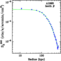
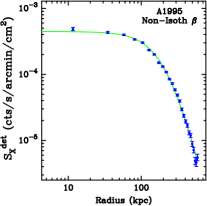
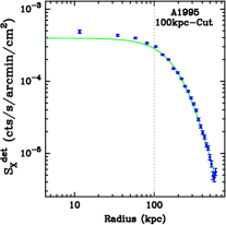
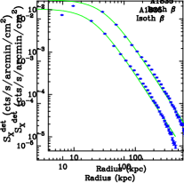
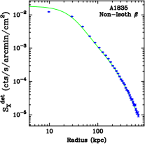
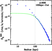
Figure 1 shows the isothermal -model, non-isothermal -model, and 100 kpc-cut model as fit to both the non cool-core cluster A1995 and the cool-core cluster A1835. The X-ray surface brightness profiles are background subtracted and constructed using concentric annuli centered on the cluster (e.g., Bonamente et al., 2006). The model fitting is done to the entire two-dimensional cluster image. Table 2 lists the spatial ( and ), spectral (isothermal spectroscopic gas temperature ), and inferred (, , ) cluster quantities obtained using these three ICM models. The radius is computed using parameters from the 100 kpc-cut models. Temperature profiles and data points for the non-isothermal models can be found in Bonamente et al. (2006), who demonstrate that the spectroscopic data are well fit by the model temperature profiles.
In the case of A1995 (a non cool-core cluster), we find that the results are largely insensitive to the chosen model. The surface brightness profiles appear well fit by all three models, and the derived gas masses, total masses, and gas mass fractions are in good agreement. Although and differ slightly, these parameters are sufficiently degenerate that the difference has a very small effect on the derived masses. These results illustrate that the simple 100 kpc-cut model works as well as the more sophisticated non-isothermal double -model for the non cool-core clusters.
Analysis of the cool-core cluster A1835, on the other hand, highlights the importance of a proper treatment of the cluster core. The most striking differences are the masses derived from the isothermal -model versus those from the other two models. This illustrates the shortcomings of a brute force application of the isothermal -model to cool-core clusters. The mass discrepancies can be attributed to a poorer fit to the surface brightness at kpc; this arises because the fit is driven mainly by the extremely high signal to noise data in the cluster core. A1835 and other cool-core clusters tend to have extremely small core radii and parameters when fit by a single isothermal -model. We also find that the X-ray spectroscopic temperature, , is biased low when the core is included in the determination of , which has an additional impact on the total mass estimate of the cluster.
The models can be quantitatively compared using a goodness of fit analysis. Goodness of fit for the X-ray data is assessed using Monte-Carlo simulations, following Winkler et al. (1995). For a given cluster, we construct the best-fit model and compare with the data to determine the fit statistic from Eq. [9]. Poisson noise is then randomly added to the best-fit model, creating new realizations, and the fit statistic is calculated for each by comparing them with the original best-fit model. The fraction of simulations that give a lower fit statistic than that of the best-fit model compared to the data is called the “goodness” (e.g., Jonker et al., 2005), with values near 0.5 indicating a good fit to the data and values near zero or one indicating a poor fit.
In the case of A1995, all three models (standard isothermal , 100 kpc-cut, and non-isothermal) provide acceptable descriptions of the data, with respective goodness values of 0.416, 0.427, and 0.496. Acceptable goodness values of 0.547, 0.548, and 0.603, for the same three models, are also found for A1835. However, the goodness value for the standard isothermal -model may be biased by the extremely high count rate in the core of this cluster. To investigate this, we use the best-fit parameters from the standard -model, but test them with the 100 kpc-cut dataset. The result is a goodness of zero; the standard -model is a poor description of the cluster gas distribution between 100 kpc and . Tests on clusters in our sample indicate that 90—95% of the cluster gas mass within lies beyond a 100 kpc radius (LaRoque, 2005). It is therefore critical that the model give a good description of the data between 100 kpc and , which the standard isothermal -model fails to do. By contrast, when the best-fit non-isothermal -model parameters are fit to the data between 100 kpc and , the goodness is 0.776, implying a much better description of the data in this region.
4.4 Testing the Model with Simulations
The ability of the 100 kpc-cut model to recover the gas mass can be further assessed by fitting the model to projected data from simulated clusters with precisely known gas masses. This test is carried out using cosmological simulations of galaxy clusters generated with the Adaptive Refinement Tree (ART) N-body+gasdynamics code (Kravtsov, 1999; Kravtsov et al., 2002). These simulations include radiative cooling and UV heating, star formation, and stellar feedback processes in addition to the standard gas dynamics. Mock Chandra observations of these simulated clusters are performed by using the true gas density, temperature and metallicity in each gas cell along with the MEKAL spectral emissivity code (Mewe et al., 1985) to generate an energy-dependent X-ray flux between 0.1 and 10 keV. This flux is then projected along the line of sight, converted to a photon count rate appropriate for , and convolved with an instrumental response simulating that of ACIS-I between 0.7 and 7.0 keV. This generates a counts image similar to the Chandra level 2 event files described in §3. The spectroscopic temperature over a region of interest is determined using an absorbed MEKAL model in XSPEC (Nagai et al., in preparation). Temperatures derived using the MEKAL model differ by at most a few percent from those derived from the relativistic Raymond-Smith model used in our analysis. These temperatures should therefore well approximate the measured Chandra temperatures for the clusters in our sample.
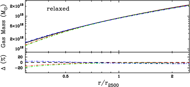
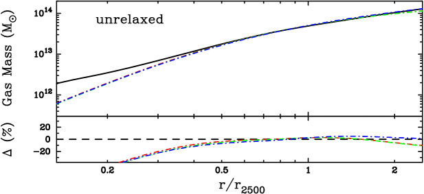
We have fit -models to the counts images described above for four different simulated clusters, spanning a range in mass from to at and including both relaxed and unrelaxed clusters. Three fits are performed for each cluster; one each to projections along three perpendicular axes. The likelihood analysis follows the methods of §4.2, and the central 100 kpc of each simulated cluster are excluded from the fit. Any obvious gas clumps are also removed from the mock images prior to fitting. A spectroscopic temperature is measured between 100 kpc and , and the masses are determined at . Goodness values for 100 kpc-cut fits to the simulated data are consistently in the range 0.35 to 0.65, implying an acceptable description of the data.
Figure 2 shows the mass results for both a highly relaxed and a highly unrelaxed cluster. In both relaxed and unrelaxed clusters, the gas mass is recovered to better than 10% between 0.5 and 2, and to better than 5% within for the twelve different fits. This shows that the simple isothermal -model with central 100 kpc excluded does an excellent job of recovering the true three-dimensional gas mass distribution from the two-dimensional projected data at radii encompassing in simulated clusters.
5 Additional Sources of Uncertainty
Before presenting the results, we discuss possible sources of both statistical and systematic uncertainty in our measurements and estimate their effects on the X-ray and SZE derived gas mass fraction in clusters. Bonamente et al. (2006) address sources of statistical and systematic uncertainty in the X-ray and SZE measurements as they apply to calculation of the angular diameter distance . Some are found to have a negligible effect on our measurements, such as uncertainties in the assumed Galactic used to calculate spectroscopic temperatures, and interference associated with other anisotropies in the CMB. However, we do review non-negligible effects discussed in Bonamente et al. (2006) in the context of the calculations, and we address additional uncertainties unique to the analysis. The effect of these uncertainties on the gas mass fractions is summarized in Table 3. The effects are quantified below in terms of their impact on the gas mass fraction for individual clusters. Note, however, that in mean results for the sample presented in §6.1, statistical uncertainties average down by a factor of one over square root of the sample size, while systematic uncertainties do not average down.
5.1 Selection Effects
Clusters chosen for SZE observation are generally selected on the basis of X-ray luminosity, . Selecting by X-ray brightness could bias the SZE sample toward elliptical clusters elongated along the line of sight; selecting instead by luminosity alleviates this problem. However, selecting by may introduce other biases because of the preferential selection of cool-core clusters or clusters undergoing major merging events. Another SZE selection bias involves point sources; preferentially selecting clusters without bright ( mJy) point sources in the field may bias our sample toward non cool-core clusters, or toward clusters at higher redshifts whose properties might differ from nearby clusters (e.g., Grego et al., 2001; Reese et al., 2002). X-ray selection biases could also be a factor, as we only include clusters which can be fit with the 100 kpc-cut and non-isothermal double -models. Three clusters, CL J0152.71357, Abell 520, and MACS J0717.5+3745, are not included in our sample due to their highly irregular morphologies.
We assess the bias associated with sample selection by attempting to construct a subsample largely free of these effects. The subsample consists of clusters from the BCS catalog (Ebeling et al., 1998), which is compiled with data from a single instrument (ROSAT) and has a well-defined flux limit of erg cm-2 s-1 in the ROSAT 0.1—2.4 keV band. The subsample contains only clusters with redshifts to minimize biases associated with cluster redshift evolution. To reduce selection effects associated with line-of-sight elongation, we impose a flux cut of erg cm-2 s-1 on the subsample, which is 50% higher than the BCS flux limit. We further select clusters with intrinsic luminosities in the range erg s-1 in the 2—10 keV Chandra band. This eliminates clusters in the extreme high and low luminosity ranges of our sample, which may have unusual dynamical properties. The final subsample consists of the ten clusters A267, A665, A773, Zw3146, A1413, A1914, A2204, A2218, A2261, and R2129 (A1413 and R2129 are not included when the SZE-only model is considered, for reasons discussed in §6.1).
To quantify the effects of selection biases, we calculate the weighted mean values using the 100 kpc-cut, non-isothermal, and SZE-only model results (see §6.1) for both the full cluster sample and the unbiased subsample. We find that the mean changes by less than 3% between the full and unbiased samples, for all three of these models. We therefore conclude that selection effects do not appear to have a substantial impact on the gas mass fraction or cosmological results.
5.2 Kinetic SZE
The kinetic SZE is a distortion in the CMB spectrum caused by the peculiar velocity of a cluster along the line of sight. Reese et al. (2002) report that, for a cluster with keV and with typical line of sight peculiar velocity of 300 km s-1 (Watkins, 1997; Colberg et al., 2000), the kinetic SZE would be 4% of the thermal SZE for our 30 GHz observations. This effect can be positive or negative depending on whether the cluster is moving toward us or away from us. Since the SZE-derived is linearly proportional to the SZE decrement, the kinetic SZE introduces a additional statistical uncertainty into the measurement of each cluster.
5.3 Radio Point Source Contamination
Point sources unaccounted for in the SZE data can cause the decrement to be “filled in” by the point source flux, diminishing the magnitude of the SZE signal. It is also possible to overestimate the magnitude of the decrement if the point source is in a negative beam sidelobe. Point sources are identified in the data using images from DIFMAP. All cluster fields are also cross-referenced with 1.4 GHz maps from the NRAO VLA Sky Survey (NVSS) (Condon et al., 1998), which occasionally allow us to distinguish faint point sources with flat or gently declining spectra from the noise in the 30 GHz maps. For cases in which NVSS shows a bright source that does not show up at 30 GHz, we place a point source model at the NVSS position and marginalize over its flux. Strongly inverted sources with 30 GHz fluxes near the noise limit would not show up in NVSS, but should be rare. Cooray et al. (1998) report spectral indices for 55 point sources with fluxes measured between 1.4 GHz and 30 GHz, finding only three with mildly inverted spectra.
NVSS contains only point sources with fluxes greater than 2 mJy at 1.4 GHz. To test the effect of point sources too faint to be cross-correlated with NVSS, LaRoque et al. (2002) randomly distribute point sources in the field of the cluster A2163 according to a number count versus flux density relationship calibrated from 41 clusters observed with BIMA. Considering undetected point sources with intrinsic fluxes between 10 Jy and 300 Jy at 30 GHz, they find that the best-fit SZE decrement can change by .
Most clusters have massive central cD galaxies, and many of them are radio bright. LaRoque et al. (2002) include a point source model at the optical position of the cD galaxy in A2163 and marginalize over its flux. They find an increase in magnitude of the best-fit central decrement of 2%, and the best-fit point source flux is consistent with zero. Reese et al. (2002) uses a similar treatment, placing point source models at the centers of the clusters A697, A2261, and A1413. The best-fit fluxes are all consistent with zero, and again increase the magnitude of by only . We conclude that the effect of undetected point sources is likely dominated by the off-center sources, and should add an additional statistical uncertainty to the SZE gas mass fractions for each cluster.
5.4 Instrument Calibration
The absolute calibration of the ACIS response is uncertain at the 5% level in the 0.7—7.0 keV band (http://cxc.harvard.edu/cal), after CTI corrections and correction for contamination on the optical blocking filters are applied. Measurements of are also subject to systematic uncertainty, owing mainly to calibration errors between energy bins. The Chandra calibration uncertainty therefore translates to uncertainty in the X-ray gas mass () and 5% in the HSE total mass () for a 6% uncertainty in the X-ray . Absolute calibration of the BIMA/OVRO interferometric imaging system is known conservatively to 4% (Reese et al., 2002), which when combined with the uncertainty in translates to a 6% systematic uncertainty in the SZE derived gas mass () and 8% systematic uncertainty in the SZE-derived .
5.5 X-ray Background
X-ray background is usually estimated from regions as far from a cluster as possible; however, due to space constraints on the chip, the background regions might contain some amount of cluster flux, particularly for low- clusters which subtend a larger solid angle on the sky. We therefore test the effect of overestimating the X-ray background due to cluster contamination on a relatively nearby cool core cluster, Zw3146. This cluster is on chip I3, so the original background is extracted from circular regions on chips I0, I1, and I2 at appropriate distances from the readouts (e.g., Bonamente et al., 2004). To assess the effect of overestimating the background, we move the extraction regions closer to the cluster until the best-fit background increases by due to cluster contamination. This should be seen as an extreme case, only applicable to a small number of bright, nearby clusters in our sample. The spectral fits are redone with these new background regions, and the resulting temperature and higher background level are applied in the X-ray/SZE joint fit.
We find that the higher X-ray background modifies the best-fit parameters, but the magnitude of the effect on individual parameters is small () with a combined effect on of . We repeat this same analysis on one of the non cool-core clusters, A2259, which has a much smaller central surface brightness to background ratio, and find that the results are much the same. Given that typical statistical uncertainty in is at most , much less than the systematic uncertainty of 25% considered here, fixing the background in our analysis should have a negligible effect on the results presented in this paper. Accounting for the fact that some clusters are more susceptible than others to an overestimated X-ray background, we add a one-sided systematic uncertainty to the X-ray derived results.
5.6 Effects of Asphericity
All cluster analysis presented in this paper uses a spherical model. Here we assess the effects of this assumption on the results presented in this paper. To assess this effect, we refit the X-ray data of all 38 clusters using a 100 kpc-cut isothermal -model and accounting for projected ellipticity and position angle of the clusters on the sky. We find a mean projected ellipticity with rms scatter 0.09, where is the ratio of a cluster’s minor axis to major axis. These results are consistent with the previous studies of Mohr et al. (1995). Accounting for the inclination angle (e.g., Cooray, 1998), an ellipsoidal cluster with and axis of symmetry inclined at to the line of sight can have a derived total mass in error by 12% and derived gas mass in error by 6% if modeled as a sphere. Extending this to the more complex triaxial distributions, we conservatively estimate a statistical uncertainty of 10% in the X-ray derived and 15% in . This translates to a statistical uncertainty in the X-ray derived gas mass fractions, given that the changes in gas mass and total mass can either add or partially cancel depending on inclination angle and geometry (Piffaretti et al., 2003). The effect on the SZE results should be smaller since the SZE depends linearly on density. Grego et al. (2000) calculate the gas mass fraction of A370 assuming both prolate and oblate geometries and find a resulting uncertainty in of 20%. This cluster has , however, so we assume a milder 10% statistical uncertainty in the SZE results for each cluster.
5.7 Hydrostatic Equilibrium
The HSE condition is a key assumption that enables measurements of the gravitationally bound mass of clusters from the X-ray and SZE data. The assumption is that the ICM is supported against gravitational collapse only by thermal pressure of the hot intracluster gas. The hydrostatic mass would therefore underestimate the true gravitational bound mass of the cluster if non-thermal pressure support is present. One form of non-thermal pressure comes from turbulent gas motions in clusters. Recent numerical simulations suggest that this provides about 10% of the total pressure support in clusters (Faltenbacher et al., 2005; Rasia et al., 2006; Lau et al., 2006) and similar results are obtained using XMM-Newton observations of the Coma cluster (Schuecker et al., 2004). More direct measurements of the turbulent gas motions in clusters, however, await measurements of Doppler broadening of the iron lines with high-resolution X-ray spectroscopy experiments (Inogamov & Sunyaev, 2003). Cosmic rays and magnetic fields may also provide non-thermal pressure support. While direct measurements of the non-thermal pressure support may be difficult, detailed comparisons of the hydrostatic mass with other mass estimates for the same cluster (e.g., gravitational lensing and the velocity dispersion of galaxies in clusters) will likely provide an important check on the hydrostatic mass estimate and potentially interesting constraints on the non-thermal pressure support in clusters. For now we assign a one-sided systematic uncertainty of to the total masses which accounts for the assumed contribution from non-thermal pressure. We caution, however, that this estimate is somewhat uncertain and this effect will need to be investigated in greater detail as more data become available.
5.8 Isothermal Assumption
The isothermal assumption can potentially affect the gas mass fraction measurements and the cosmological constraints through its effects on both gas mass and total mass. The X-ray derived gas mass is affected little by the isothermal assumption, because the X-ray emission has a very weak dependence on the assumed temperature (). The SZE derived gas mass is more sensitive to this assumption since it depends linearly on the cluster gas temperature. Our choice of a radial range between 100 kpc and should minimize the bias due to the temperature structure for two reasons: (1) use of the X-ray temperature with the 100 kpc core exclusion should avoid the most significant bias associated with cool-core clusters, and (2) focusing on the inner should minimize the bias due to the temperature decline observed in the outskirts of clusters (Vikhlinin, 2005).
The total mass derived from the X-ray and SZE data is also affected by the isothermal assumption. If the temperature profile deviates from the isothermal gas distribution, the average temperature depends on the weighting scheme. For example, the spectroscopic temperature, , may differ by about 10% from the gas mass-weighted temperature in the radial range between 70 kpc and (Vikhlinin, 2005). But the difference is likely smaller in the radial range (100 kpc ) considered in this study. We therefore expect that the bias on the cluster masses and hence our gas mass fraction measurements is not significant.
The effect of the isothermal assumption can be quantified using the results of Table 7, presented in §6.1 below. There we find that the X-ray and SZE weighted mean gas mass fractions are nearly identical for the non-isothermal model, while the SZE gas mass fraction is larger than the X-ray value for the 100 kpc-cut model. This hints at a possible systematic bias of about in the spectral temperature under the isothermal assumption, since the SZE has an additional dependence relative to the X-ray. We therefore assign an additional systematic uncertainty to the gas mass fractions derived from the X-ray 100 kpc-cut fits, and a systematic uncertainty to the gas mass fractions from the SZE 100 kpc-cut fits.
5.9 Cluster Substructure
The X-ray derived gas mass fractions are particularly sensitive to any non-negligible small scale structure in the intracluster gas. When gas clumps, it has density higher than the local average, , and the X-ray surface brightness is increased by a factor of relative to the SZE decrement (Nagai et al., 2000; Mathiesen & Evrard, 2001). Since for the X-ray data and for the SZE data, X-ray gas mass fractions would be systematically overestimated by a factor of with respect to SZE gas mass fractions in the presence of significant clumping. Cluster substructure has two important effects on the X-ray observables. First, gas clumps can bias the measured X-ray gas mass high by . Second, cluster substructure can bias the average spectroscopic temperature of the cluster as a whole (e.g., Mathiesen & Evrard, 2001; Mazzotta et al., 2004).
The Chandra observations provide important handles on both of these effects, because their superb resolution and sensitivity enable detection of the prominent clumps that contribute significantly to the X-ray surface brightness and the determination of the average temperature of the cluster. We test this using the mock Chandra observations of the simulated clusters introduced in §4.4. The test shows that the gas mass is recovered to better than 5% using the simple 100 kpc-cut model, indicating that the clumping factor should be small if the most prominent clump is removed from the image. These results should also hold for the high clusters, as a significant fraction of the low energy photons from the cool clumps are redshifted out of the 0.7—7 keV band, making the instrument less sensitive to clumping effects (Nagai et al., in preparation).
For the same reasons, the bias on the Chandra spectroscopic temperature is also small. Tests on several clusters in our sample show that not removing bright clumps may bias the temperatures low by 10—15%, in reasonable agreement with the previous findings (Mathiesen & Evrard, 2001; Mazzotta et al., 2004). Further tests, leaving in only fainter clumps, show a decrease in spectroscopic temperature of only 2—3%, smaller than the assumed bias due to the isothermal assumption.
We therefore conclude that there is no evidence that cluster substructure significantly affects our results when bright spots are removed from the X-ray images prior to fitting. The agreement in the mean X-ray and SZE gas mass fractions, particularly for the non-isothermal model which avoids the bias due to the isothermal assumption, is consistent with this conclusion (cf. §6.3).
6 Results and Discussion
6.1 Gas Mass Fraction Results
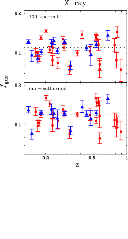
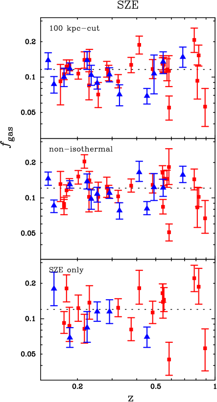
In Table 4 we present the X-ray and SZE measurements of cluster gas mass fractions as determined from the 100 kpc-cut model (§4.1.1). The X-ray and SZE data are fit jointly, with the cluster core radius and parameter linked between datasets while the central surface brightness and central SZE decrement are allowed to vary. The gas mass fractions are plotted as a function of redshift in Figure 3. X-ray surface brightness profiles and the best-fit 100 kpc-cut models are shown in Appendix A for the 38 clusters in our sample. The X-ray surface brightness profiles are well described by the isothermal -model beyond 100 kpc from the cluster center.
In Table 5 we present X-ray and SZE gas mass fractions determined from the non-isothermal model (§4.1.2). The X-ray and SZE data are again fit jointly with shape parameters linked, while the X-ray and SZE central density parameters are allowed to vary separately. The gas mass fractions are plotted as a function of redshift in Figure 3. Surface brightness profiles for the non-isothermal model are shown in Bonamente et al. (2006), and show consistently good fits to the cluster radial profiles out to .
In Table 6 we present SZE gas mass fractions determined from the SZE-only model (§4.1.3). We find that this model constrains and individually in 23 of our 38 clusters, and those 23 are shown in the table. Gas mass fractions derived with this method are plotted versus redshift in Figure 3.
The mean X-ray and SZE gas mass fractions for all three models are summarized in Table 7, where the uncertainties are statistical followed by systematic at 68% confidence. The statistical uncertainties include the effects of cluster asphericity, radio point sources, and the kinetic SZE, combined in quadrature; systematic uncertainties include errors associated with instrument calibration, X-ray background, and the assumptions of HSE and isothermality (see §5 and Table 3). The results show that the X-ray and SZE measurements of the mean gas mass fraction in clusters agree to better than 10% for the three ICM models considered.
6.2 Effects of Cluster Cores on Derived Gas Mass Fractions
The results summarized in Table 7 show that the X-ray and SZE derived gas mass fractions agree remarkably well as long as care is taken to account for the effect of the cluster core on the X-ray emission. The results show that the core can be satisfactorily accounted for by either ignoring the core in fits to the X-ray data (the 100 kpc-cut model) or modeling the ICM with the non-isothermal double- model.
It is also noteworthy that the gas mass fraction results derived from spatial fits to only the SZE data including the core also agree remarkably well with the above models. This indicates that the SZE is not very sensitive to the cluster core, and is in line with expectations since the SZE is a probe of the ICM pressure.
The effect of cluster cores on the gas mass fractions is further investigated by comparing results for cool-core and non cool-core subsamples. There is a population of clusters in our sample with bright and sharply peaked cores (cf. Appendix A), including A586, MC0744, Zw3146, A1413, MC1311, A1689, R1347, MS1358, A1835, MC1423, A2204, A2261, and R2129. These clusters have central cooling times (calculated with the cores included in the X-ray data) less than 0.5 , and we refer to this subsample as the cool-core sample because the sharply peaked X-ray emission is indicative of strong radiative cooling in the cluster core. The results of a comparison of cool-core and non cool-core weighted mean gas mass fractions are shown in Table 8, where in addition to the three main ICM models considered above, we include results from two additional naive models which make no effort to compensate for the cluster cores: (1) a no-cut isothermal -model fit jointly to the full X-ray and SZE datasets, and (2) a spatial model fit to only the SZE data as before, but using the X-ray temperature derived from all of the X-ray data instead of the data with central 100 kpc excluded.
Apart from a small % offset in the X-ray results, the derived gas mass fractions for the 100 kpc-cut and non-isothermal models for the cool-core and non cool-core clusters are in excellent agreement. Figure 3 also demonstrates this agreement, as there is no systematic offset seen between the cool-core (triangles) and non cool-core (squares) clusters. The results for the naive models clearly show the importance of accounting for the core in the cool-core subsample; large offsets are found for the derived gas mass fraction of the cool-core subsample, while the same naive models provide perfectly consistent results for the non cool-core subsample. The primary cause of the biased results of the naive models for the cool-core clusters is the poor spatial fits and the low . A depressed results in a lower derived total cluster mass as well as a higher SZE gas mass.
6.3 Constraints on Clumping in the Intracluster Gas
The comparison of the X-ray and SZE gas mass fraction measurements shows that the results are in good agreement. These results suggest a clumping factor of the ICM consistent with zero. The high resolution Chandra data allow one to remove any visible clumps before the data are fit, and the agreement between X-ray and SZE gas mass fraction measurements indicates that any clumps below the noise level of the data have a negligible effect on the mass measurements. Further indications in favor of a negligible clumping factor are discussed in §5.9.
6.4 Comparison with previous studies
Finally, we compare our X-ray and SZE gas mass measurements to the results from previous studies in the literature. We first compare our X-ray results with Chandra results obtained using a different analysis technique (Allen et al., 2002, 2004)111Although mean gas mass fraction results for other cluster samples are available in the literature (e.g., Evrard, 1997; Mohr et al., 1999; Ettori et al., 2003; Sanderson et al., 2003), the detailed comparisons with our results are non-trivial as they are often calculated at different radii and assume different cosmologies., in which the cluster mass is modeled assuming that the cluster gas is in hydrostatic equilibrium with a NFW potential and using a deprojected 3D gas temperature profile. These authors report mean gas mass fractions of for a sample of six highly relaxed clusters (Allen et al., 2002) and for a larger sample of 26 relaxed clusters (Allen et al., 2004); these results are in good agreement with our own. We also compare the results of eight clusters we have in common with the Allen et al. (2004) dataset and find that the measurements of individual clusters are consistent with no systematic offset.
For the SZE gas mass fractions, we compare results of our SZE-only model fitting directly with the results of Grego et al. (2001). There are many similarities between our cluster sample and analysis method and those of Grego et al.; for instance, they use BIMA and OVRO data, and 13 of our 23 clusters have data in common with their sample. They also use an isothermal -model to analyze the SZE data. Their approach also differs somewhat from ours, in that they (1) use spectroscopic temperatures from the literature (generally from ASCA), and (2) measure the gas mass fraction at from the cluster center, then scale the results to using relations calibrated from numerical simulations (Evrard et al., 1996; Evrard, 1997). Despite these differences, Grego et al. measure a mean gas mass fraction of , which is equivalent to for , in good agreement with our SZE derived gas mass fraction (cf. Table 7). Similarly, if we calculate gas mass fractions from our SZE-only model at 65″ and scale to using the same relations, we obtain a weighted mean of , in good agreement with the Grego et al. results. The cluster gas mass fraction results derived from the implied SZE for nearby clusters obtained from correlating known clusters with WMAP data is also consistent with our results (Afshordi et al., 2005).
7 Constraints on Cluster Physics and Cosmology
7.1 The cluster baryon budget
Currently, the relation between and the cosmological baryon fraction / is not accurately known (Ettori et al., 2006). However, since recent CMB studies provide precise constraints on cosmological parameters (e.g., Spergel et al., 2006), we can use our measurements to obtain constraints on the ratio
| (16) |
Combining our results with the WMAP values of and (, ) and the Hubble Space Telescope measurement of (Freedman et al., 2001), we obtain the constraints on given in Table 9, where uncertainties are again statistical followed by systematic at 68% confidence. Since the data are calculated assuming =0.3, =0.7, , very similar to the WMAP constraints, no significant bias is expected in the results of Table 9. These results indicate that the ratio of the gas mass fraction in clusters within to the cosmic baryon fraction, , is where the range includes statistical and systematic uncertainties, in accord with the conclusions reached by Afshordi et al. (2005). This ratio provides a benchmark for simulations of galaxy clusters. We note that recent numerical simulations that include radiative cooling and star formation have baryon budgets in line with our results, although they find that the gas tends to overcool in the cluster cores (Kravtsov et al., 2005).
7.2 Cosmological Parameters
Cluster gas mass fractions can provide strong constraints on cosmological parameters. The normalization of the cluster gas mass fraction depends sensitively on the ratio of / (e.g., White et al., 1993; David et al., 1995; Myers et al., 1997; Mohr et al., 1999; Ettori & Fabian, 1999; Grego et al., 2001; Allen et al., 2002), while the redshift evolution of the gas mass fraction depends sensitively on , and even the equation of dark energy, (Sasaki, 1996; Pen, 1997; Allen et al., 2004). Methods involving the normalization, however, depend sensitively on a priori knowledge of the cluster baryon budget which, as discussed in § 7.1, is poorly known. By contrast, methods using the redshift evolution are powerful in that they are independent of the cluster baryon budget and even prior knowledge on other cosmological parameters such as and .
We therefore consider constraints on cosmological parameters from the redshift evolution of the cluster gas mass fraction. For parameter estimation, we follow the procedure described in Allen et al. (2004), and fit the data to the model,
| (17) |
where we assume a CDM cosmology with =0.3, =0.7, as a fiducial cosmology, indicated by “fid”. Using this model, we fit an arbitrary normalization , and grid the variables and between 0 and 1.3 with the WMAP constraint (Spergel et al., 2006). We cannot place useful constraints on and from the X-ray or SZE data without a prior on the total density parameter.
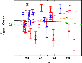
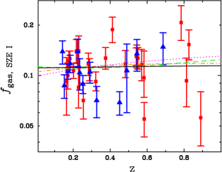
Marginalizing over the WMAP total density prior, we find best-fit parameters of , from the 100 kpc-cut X-ray data and and from the isothermal model analysis. Similarly, the non-isothermal model returns , from X-ray and , from SZE. Our results are consistent with independent tests, such as those of WMAP, and inconsistent with a matter dominated universe (=1, =0) model. In Figure 4 we show the data, the best-fit model using the WMAP prior (solid line), the best-fit model without the WMAP prior (unconstrained; dashed line), and the model corresponding to two other fiducial cosmologies (=1, =0: dotted line; =0.3, =0: dash-dotted line). Only the 100 kpc-cut results are plotted for simplicity. It is evident that the X-ray data disfavors the flat, matter-dominated model. Interestingly, systematic uncertainty should be negligible compared to statistical uncertainty with this method, since most of the systematic uncertainties affect the normalization and do not introduce trends with redshift. Cosmological constraints from this method are therefore expected to improve as the cluster sample size is increased.
8 Conclusions
We have presented X-ray and SZE measurements of gas mass fractions for a sample of 38 massive galaxy clusters using Chandra X-ray observations and BIMA/OVRO SZE radio interferometric observations. Three models for the cluster gas distributions are used in the gas mass fraction derivations: (1) an isothermal -model fit to the X-ray data at radii beyond 100 kpc and to all of the SZE data, (2) a non-isothermal double -model fit to all of the X-ray and SZE data, and (3) an isothermal -model fit to the SZE spatial data with fixed at 0.7 and a spectral temperature from the 100 kpc-cut X-ray data.
The cluster gas distributions are well fit by the non-isothermal model out to . We have also demonstrated that the simple 100 kpc-cut isothermal model provides a good description of the intracluster medium (ICM) outside of the cluster core for objects with a wide range of morphological properties.
For all three models, the mean gas mass fractions determined from the X-ray and SZE data are in excellent agreement. Specifically, with the isothermal -model we find a mean X-ray gas mass fraction (X-ray) and a mean SZE gas mass fraction (SZE), where uncertainties are statistical followed by systematic at 68% confidence. For the non-isothermal double -model, the mean gas mass fractions are (X-ray) and (SZE). For the SZE-only model, (SZE).
It is noteworthy that the gas mass fractions derived from spatial fits to only the SZE data including the core also agree remarkably well with the other models. This indicates that the SZE is largely insensitive to structure in the cluster core. The lack of sensitivity to the core structure is expected since the SZE is a probe of the gas pressure; this is promising for extracting cosmology from upcoming large scale SZE cluster surveys (e.g., see Carlstrom et al., 2002).
To investigate the effect of the cluster cores on the results, we divided the cluster sample into two subsamples depending on whether or not the clusters exhibit cool cores. The three ICM models above lead to consistent gas mass fraction results for each subsample. However, when the subsamples are fitted with naive ICM models that make no effort to account for the cluster cores, the resulting gas mass fractions for the cool-core subsample show large offsets from the above results, while the results for the non cool-core clusters are consistent with the above results. This clearly indicates the importance of accounting for the cores in clusters that exhibit cool cores.
Understanding the baryon budget in clusters is one of the most important aspects of cluster physics. Our X-ray and SZE measurements indicate that the ratio of the gas mass fraction within to the cosmic baryon fraction, , is where the range includes statistical and systematic uncertainties at 68% confidence. This result is in accord with the conclusions reached by Afshordi et al. (2005). The measurement provides a benchmark for simulations of galaxy clusters. We note that recent numerical simulations that include radiative cooling and star formation have baryon budgets in line with our measurements, although they find that the gas tends to overcool in the cluster cores (Kravtsov et al., 2005).
Our results also have implications for cosmological constraints based on measurements of cluster gas mass fractions. Constraints from the normalization of the gas mass fraction depend sensitively on a priori knowledge of the cluster baryon budget , which, as discussed above, is still somewhat uncertain. However, a cosmological test based on the redshift evolution of the gas mass fraction is independent of the cluster baryon budget and even prior knowledge of cosmological parameters such as and . Marginalizing over the WMAP total density prior, we use this method and find best-fit parameters of , and , from the 100 kpc-cut X-ray and SZE samples, and , and , from the non-isothermal X-ray and SZE samples, respectively. Our results are consistent with standard CDM cosmology, and inconsistent with =1, =0. Interestingly, the systematic uncertainty for this method is negligible compared to statistical uncertainty, as most sources of systematic uncertainty are not expected to introduce trends with redshift. Cosmological constraints using this method are therefore expected to improve rapidly as the cluster sample size increases with upcoming X-ray and SZE cluster surveys.
References
- Afshordi et al. (2005) Afshordi, N., Lin, Y.-T., & Sanderson, A. J. R. 2005, ApJ, 629, 1
- Allen et al. (1992) Allen, S. W. et al. 1992, MNRAS, 259, 67
- Allen et al. (2004) Allen, S. W., Schmidt, R. W., Ebeling, H., Fabian, A. C., & van Speybroeck, L. 2004, MNRAS, 353, 457
- Allen et al. (2002) Allen, S. W., Schmidt, R. W., & Fabian, A. C. 2002, MNRAS, 334, L11
- Arnaud (1996) Arnaud, K. A. 1996, in Astronomical Data Analysis Software and Systems V, ed. G. H. Jacoby & J. Barnes, 17
- Bahcall & Fan (1998) Bahcall, N. A., & Fan, X. 1998, ApJ, 504, 1
- Birkinshaw et al. (1991) Birkinshaw, M., Hughes, J. P., & Arnaud, K. A. 1991, ApJ, 379, 466
- Böhringer et al. (2000) Böhringer, H. et al. 2000, ApJS, 129, 435
- Bonamente et al. (2004) Bonamente, M., Joy, M. K., Carlstrom, J. E., Reese, E. D., & LaRoque, S. J. 2004, ApJ, 614, 56
- Bonamente et al. (2006) Bonamente, M., Joy, M. K., LaRoque, S. L., Carlstrom, J., Reese, E. D., & Dawson, K. S. 2006, ApJ, in press
- Borgani et al. (2004) Borgani, S. et al. 2004, MNRAS, 348, 1078
- Carlstrom et al. (2002) Carlstrom, J. E., Holder, G. P., & Reese, E. D. 2002, ARA&A, 40, 643
- Carlstrom et al. (1996) Carlstrom, J. E., Joy, M., & Grego, L. 1996, ApJ, 456, L75
- Cash (1979) Cash, W. 1979, ApJ, 228, 939
- Cavaliere & Fusco-Femiano (1976) Cavaliere, A., & Fusco-Femiano, R. 1976, A&A, 49, 137
- Cavaliere & Fusco-Femiano (1978) —. 1978, A&A, 70, 677
- Colberg et al. (2000) Colberg, J. M., White, S. D. M., MacFarland, T. J., Jenkins, A., Pearce, F. R., Frenk, C. S., Thomas, P. A., & Couchman, H. M. P. 2000, MNRAS, 313, 229
- Condon et al. (1998) Condon, J. J., Cotton, W. D., Greisen, E. W., Yin, Q. F., Perley, R. A., Taylor, G. B., & Broderick, J. J. 1998, AJ, 115, 1693
- Cooray (1998) Cooray, A. R. 1998, A&A, 339, 623
- Cooray et al. (1998) Cooray, A. R., Grego, L., Holzapfel, W. L., Joy, M., & Carlstrom, J. E. 1998, AJ, 115, 1388
- David et al. (1995) David, L. P., Jones, C., & Forman, W. 1995, ApJ, 445, 578
- Dickey & Lockman (1990) Dickey, J. M., & Lockman, F. J. 1990, ARA&A, 28, 215
- Donahue et al. (1998) Donahue, M., Voit, G. M., Gioia, I., Lupino, G., Hughes, J. P., & Stocke, J. T. 1998, ApJ, 502, 550
- Donahue et al. (1999) Donahue, M., Voit, G. M., Scharf, C. A., Gioia, I. M., Mullis, C. R., Hughes, J. P., & Stocke, J. T. 1999, ApJ, 527, 525
- Ebeling et al. (1998) Ebeling, H., Edge, A. C., Bohringer, H., Allen, S. W., Crawford, C. S., Fabian, A. C., Voges, W., & Huchra, J. P. 1998, MNRAS, 301, 881
- Ebeling et al. (2001) Ebeling, H., Jones, L. R., Fairley, B. W., Perlman, E., Scharf, C., & Horner, D. 2001, ApJ, 548, L23
- Elbaz et al. (1995) Elbaz, D., Arnaud, M., & Böhringer, H. 1995, A&A, 293, 337
- Ettori et al. (2006) Ettori, S., Dolag, K., Borgani, S., & Murante, G. 2006, MNRAS, 365, 1021
- Ettori & Fabian (1999) Ettori, S., & Fabian, A. C. 1999, MNRAS, 305, 834
- Ettori et al. (2004) Ettori, S., Tozzi, P., Borgani, S., & Rosati, P. 2004, A&A, 417, 13
- Ettori et al. (2003) Ettori, S., Tozzi, P., & Rosati, P. 2003, A&A, 398, 879
- Evrard (1997) Evrard, A. E. 1997, MNRAS, 292, 289
- Evrard et al. (1996) Evrard, A. E., Metzler, C. A., & Navarro, J. F. 1996, ApJ, 469, 494
- Faltenbacher et al. (2005) Faltenbacher, A., Kravtsov, A. V., Nagai, D., & Gottlöber, S. 2005, MNRAS, 358, 139
- Feldman (1992) Feldman, U. 1992, Physica Scripta Volume T, 46, 202
- Freedman et al. (2001) Freedman, W. L. et al. 2001, ApJ, 553, 47
- Gioia & Luppino (1994) Gioia, I. M., & Luppino, G. A. 1994, ApJS, 94, 583
- Grego et al. (2000) Grego, L., Carlstrom, J. E., Joy, M. K., Reese, E. D., Holder, G. P., Patel, S., Cooray, A. R., & Holzapfel, W. L. 2000, ApJ, 539, 39
- Grego et al. (2001) Grego, L., Carlstrom, J. E., Reese, E. D., Holder, G. P., Holzapfel, W. L., Joy, M. K., Mohr, J. J., & Patel, S. 2001, ApJ, 552, 2
- Henry et al. (1997) Henry, J. P. et al. 1997, AJ, 114, 1293
- Inogamov & Sunyaev (2003) Inogamov, N. A., & Sunyaev, R. A. 2003, Astronomy Letters, 29, 791
- Itoh et al. (1998) Itoh, N., Kohyama, Y., & Nozawa, S. 1998, ApJ, 502, 7
- Jones & Forman (1984) Jones, C., & Forman, W. 1984, ApJ, 276, 38
- Jones & Forman (1999) —. 1999, ApJ, 511, 65
- Jonker et al. (2005) Jonker, P. G., Campana, S., Steeghs, D., Torres, M. A. P., Galloway, D. K., Markwardt, C. B., Chakrabarty, D., & Swank, J. 2005, MNRAS, 537
- Kneissl et al. (2001) Kneissl, R., Jones, M. E., Saunders, R., Eke, V. R., Lasenby, A. N., Grainge, K., & Cotter, G. 2001, MNRAS, 328, 783
- Kosowsky (2003) Kosowsky, A. 2003, New Astronomy Review, 47, 939
- Kravtsov (1999) Kravtsov, A. V. 1999, PhD thesis, New Mexico State University
- Kravtsov et al. (2002) Kravtsov, A. V., Klypin, A., & Hoffman, Y. 2002, ApJ, 571, 563
- Kravtsov et al. (2005) Kravtsov, A. V., Nagai, D., & Vikhlinin, A. A. 2005, ApJ, 625, 588
- LaRoque (2005) LaRoque, S. J. 2005, PhD thesis, University of Chicago
- LaRoque et al. (2003) LaRoque, S. J. et al. 2003, ApJ, 583, 559
- LaRoque et al. (2002) LaRoque, S. J., Reese, E. D., Carlstrom, J. E., Holder, G., Holzapfel, W. L., Joy, M., & Grego, L. 2002, astro-ph/0204134
- Lau et al. (2006) Lau, E., Kravtsov, A. V., & Nagai, D. 2006, ApJ in preparation
- Luppino & Gioia (1995) Luppino, G. A., & Gioia, I. M. 1995, ApJ, 445, L77
- Mathiesen & Evrard (2001) Mathiesen, B. F., & Evrard, A. E. 2001, ApJ, 546, 100
- Mazzotta et al. (2004) Mazzotta, P., Rasia, E., Moscardini, L., & Tormen, G. 2004, MNRAS, 354, 10
- Mewe et al. (1985) Mewe, R., Gronenschild, E. H. B. M., & van den Oord, G. H. J. 1985, A&AS, 62, 197
- Mohr et al. (1995) Mohr, J. J., Evrard, A. E., Fabricant, D. G., & Geller, M. J. 1995, ApJ, 447, 8
- Mohr et al. (1999) Mohr, J. J., Mathiesen, B., & Evrard, A. E. 1999, ApJ, 517, 627
- Myers et al. (1997) Myers, S. T., Baker, J. E., Readhead, A. C. S., Leitch, E. M., & Herbig, T. 1997, ApJ, 485, 1
- Nagai (2005) Nagai, D. 2005, ApJ– submitted: astro-ph/0512208
- Nagai et al. (2000) Nagai, D., Sulkanen, M. E., & Evrard, A. E. 2000, MNRAS, 316, 120
- Navarro et al. (1996) Navarro, J. F., Frenk, C. S., & White, S. D. M. 1996, ApJ, 462, 563
- Navarro et al. (1997) —. 1997, ApJ, 490, 493
- Patel et al. (2000) Patel, S. K. et al. 2000, ApJ, 541, 37
- Pearson et al. (1994) Pearson, T. J., Shepherd, M. C., Taylor, G. B., & Myers, S. T. 1994, BAAS, 185, 0808
- Pen (1997) Pen, U. 1997, New Astronomy, 2, 309
- Perlmutter et al. (1999) Perlmutter, S. et al. 1999, ApJ, 517, 565
- Piffaretti et al. (2003) Piffaretti, R., Jetzer, P., & Schindler, S. 2003, A&A, 398, 41
- Rasia et al. (2006) Rasia, E. et al. 2006, MNRAS—submitted: astro-ph/0602434
- Raymond & Smith (1977) Raymond, J. C., & Smith, B. W. 1977, ApJS, 35, 419
- Reese et al. (2002) Reese, E. D., Carlstrom, J. E., Joy, M., Mohr, J. J., Grego, L., & Holzapfel, W. L. 2002, ApJ, 581, 53
- Reese et al. (2000) Reese, E. D. et al. 2000, ApJ, 533, 38
- Riess et al. (1998) Riess, A. G. et al. 1998, AJ, 116, 1009
- Romer et al. (2001) Romer, A. K., Viana, P. T. P., Liddle, A. R., & Mann, R. G. 2001, ApJ, 547, 594
- Rudy (1987) Rudy, D. J. 1987, PhD thesis, California Institute of Technology
- Ruhl et al. (2004) Ruhl, J. E. et al. 2004, astro-ph/0411122
- Sanderson & Ponman (2003) Sanderson, A. J. R., & Ponman, T. J. 2003, MNRAS, 345, 1241
- Sanderson et al. (2003) Sanderson, A. J. R., Ponman, T. J., Finoguenov, A., Lloyd-Davies, E. J., & Markevitch, M. 2003, MNRAS, 340, 989
- Sarazin (1988) Sarazin, C. L. 1988, X-ray Emission From Clusters of Galaxies (Cambridge University Press)
- Sasaki (1996) Sasaki, S. 1996, PASJ, 48, L119
- Sault et al. (1995) Sault, R. J., Teuben, P. J., & Wright, M. C. H. 1995, in Astronomical Data Analysis Software and Systems IV, ed. R. A. Shaw, H. E. Payne, & J. J. E. Hayes, 433
- Schindler et al. (1995) Schindler, S. et al. 1995, A&A, 299, L9
- Schuecker et al. (2004) Schuecker, P., Finoguenov, A., Miniati, F., Böhringer, H., & Briel, U. G. 2004, A&A, 426, 387
- Scoville et al. (1993) Scoville, N. Z., Carlstrom, J. E., Chandler, C. J., Phillips, J. A., Scott, S. L., Tilanus, R. P. J., & Wang, Z. 1993, PASP, 105, 1482
- Spergel et al. (2006) Spergel, D. N. et al. 2006, ApJ—submitted: astro-ph/0603449
- Stocke et al. (1991) Stocke, J. T., Morris, S. L., Gioia, I. M., Maccacaro, T., Schild, R., Wolter, A., Fleming, T. A., & Henry, J. P. 1991, ApJS, 76, 813
- Struble & Rood (1999) Struble, M. F., & Rood, H. J. 1999, ApJS, 125, 35
- Sunyaev & Zel’dovich (1970) Sunyaev, R. A., & Zel’dovich, Y. B. 1970, Comments Astrophys. Space Phys., 2, 66
- Sunyaev & Zel’dovich (1972) —. 1972, Comments Astrophys. Space Phys., 4, 173
- Vikhlinin (2005) Vikhlinin, A. 2005, ApJ—submitted: astro-ph/0504098
- Vikhlinin et al. (2005) Vikhlinin, A., Kravtsov, A., Forman, W., Jones, C., Markevitch, M., Murray, S. S., & Van Speybroeck, L. 2005, ApJ—submitted: astro-ph/0507092
- Watkins (1997) Watkins, R. 1997, MNRAS, 292, L59
- White et al. (1993) White, S. D. M., Navarro, J. F., Evrard, A. E., & Frenk, C. S. 1993, Nature, 366, 429
- Winkler et al. (1995) Winkler, C. et al. 1995, A&A, 302, 765
| Chandra X-ray Data | Interferometric SZE Data | ||||||||||
|---|---|---|---|---|---|---|---|---|---|---|---|
| Cluster | z | ObsID | Chip | (ks) | (hh mm ss) | ( ) | BIMA (hr) | OVRO (hr) | (hh mm ss) | ( ) | reference |
| CL 0016+1609 | 0.541 | 520 | I3 | 67.4 | 00 18 33.5 | +16 26 12.5 | 43 | 100 | 00 18 33.3 | +16 26 04.0 | Stocke et al. (1991) |
| ABELL 68 | 0.255 | 3250 | I3 | 10.0 | 00 37 06.2 | +09 09 33.2 | 54 | – | 00 37 04.0 | +09 10 02.5 | Struble & Rood (1999) |
| ABELL 267 | 0.230 | 1448 | I3 | 7.4 | 01 52 42.1 | +01 00 35.7 | 50 | – | 01 52 42.3 | +01 00 26.0 | Struble & Rood (1999) |
| ABELL 370 | 0.375 | 515 | S3 | 65.3 | 02 39 53.2 | -01 34 35.0 | 26 | 33 | 02 39 52.4 | -01 34 43.8 | Struble & Rood (1999) |
| MS 0451.6-0305 | 0.550 | 902 | S3 | 42.2 | 04 54 11.4 | -03 00 52.7 | – | 30 | 04 54 11.6 | -03 01 01.3 | Gioia & Luppino (1994) |
| 529 | I3 | 13.9 | |||||||||
| MACS J0647.7+7015 | 0.584 | 3196 | I3 | 19.3 | 06 47 50.2 | +70 14 54.6 | – | 23 | 06 47 50.2 | +70 14 56.1 | LaRoque et al. (2003) |
| 3584 | I3 | 20.0 | |||||||||
| ABELL 586 | 0.171 | 530 | I3 | 10.0 | 07 32 20.2 | +31 37 55.6 | 45 | – | 07 32 19.6 | +31 37 55.3 | Struble & Rood (1999) |
| MACS J0744.8+3927 | 0.686 | 3197 | I3 | 20.2 | 07 44 52.8 | +39 27 26.7 | 8 | 17 | 07 44 52.4 | +39 27 33.2 | LaRoque et al. (2003) |
| 3585 | I3 | 19.4 | |||||||||
| ABELL 611 | 0.288 | 3194 | S3 | 36.1 | 08 00 56.6 | +36 03 24.1 | – | 57 | 08 00 56.5 | +36 03 22.9 | Struble & Rood (1999) |
| ABELL 665 | 0.182 | 3586 | I3 | 29.7 | 08 30 58.1 | +65 50 51.6 | 52 | 16 | 08 30 58.6 | +65 50 49.8 | Struble & Rood (1999) |
| 531 | I3 | 9.0 | |||||||||
| ABELL 697 | 0.282 | 4217 | I3 | 19.5 | 08 42 57.5 | +36 21 56.2 | – | 47 | 08 42 57.8 | +36 21 54.5 | Struble & Rood (1999) |
| ABELL 773 | 0.217 | 533 | I3 | 11.3 | 09 17 52.8 | +51 43 38.9 | 26 | 66 | 09 17 53.5 | +51 43 49.8 | Struble & Rood (1999) |
| 3588 | I3 | 9.4 | |||||||||
| ZW 3146 | 0.291 | 909 | I3 | 46.0 | 10 23 39.7 | +04 11 09.5 | 25 | 15 | 10 23 37.8 | +04 11 17.8 | Allen et al. (1992) |
| MS 1054.5-0321 | 0.826 | 512 | S3 | 89.1 | 10 56 59.4 | -03 37 34.2 | – | 43 | 10 56 59.1 | -03 37 34.0 | Luppino & Gioia (1995) |
| MS 1137.5+6625 | 0.784 | 536 | I3 | 77.0 | 11 40 22.3 | +66 08 16.0 | 88 | – | 11 40 23.1 | +66 08 05.3 | Donahue et al. (1999) |
| MACS J1149.5+2223 | 0.544 | 1656 | I3 | 18.5 | 11 49 35.5 | +22 24 02.3 | 39 | – | 11 49 34.9 | +22 23 54.8 | LaRoque et al. (2003) |
| 3589 | I3 | 20.0 | |||||||||
| ABELL 1413 | 0.142 | 1661 | I3 | 9.7 | 11 55 18.0 | +23 24 17.0 | 28 | – | 11 55 17.7 | +23 24 39.5 | Struble & Rood (1999) |
| 537 | I3 | 9.6 | |||||||||
| CL J1226.9+3332 | 0.890 | 3180 | I3 | 31.7 | 12 26 57.9 | +33 32 47.4 | 33 | – | 12 26 58.0 | +33.32 57.9 | Ebeling et al. (2001) |
| 932 | S3 | 9.9 | |||||||||
| MACS J1311.0-0310 | 0.490 | 3258 | I3 | 14.9 | 13 11 01.7 | -03 10 38.5 | 39 | – | 13 11 02.2 | -03 10 45.6 | Allen et al. (2004) |
| ABELL 1689 | 0.183 | 1663 | I3 | 10.7 | 13 11 29.5 | -01 20 28.2 | 16 | 26 | 13 11 29.1 | -01 20 29.7 | Struble & Rood (1999) |
| 540 | I3 | 10.3 | |||||||||
| RX J1347.5-1145 | 0.451 | 3592 | I3 | 57.7 | 13 47 30.6 | -11 45 08.6 | 22 | 3 | 13 47 30.6 | -11 45 12.3 | Schindler et al. (1995) |
| MS 1358.4+6245 | 0.327 | 516 | S3 | 48.1 | 35 59 50.6 | +62 31 04.1 | 70 | – | 13 59 50.2 | +62 31 07.0 | Gioia & Luppino (1994) |
| ABELL 1835 | 0.252 | 495 | S3 | 19.5 | 14 01 02.0 | +02 52 41.7 | 27 | 23 | 14 01 01.8 | +02 52 45.6 | Struble & Rood (1999) |
| 496 | S3 | 10.7 | |||||||||
| MACS J1423.8+2404 | 0.545 | 4195 | S3 | 115.6 | 14 23 47.9 | +24 04 42.6 | 35 | – | 14 23 47.7 | +24 04 37.3 | LaRoque et al. (2003) |
| ABELL 1914 | 0.171 | 3593 | I3 | 18.9 | 14 26 00.8 | +37 49 35.7 | 24 | – | 14 26 01.3 | 37 49 38.6 | Struble & Rood (1999) |
| 542 | I3 | 8.1 | |||||||||
| ABELL 1995 | 0.322 | 906 | S3 | 56.7 | 14 52 57.9 | +58 02 55.8 | 50 | 58 | 14 52 58.1 | +58 02 57.0 | Patel et al. (2000) |
| ABELL 2111 | 0.229 | 544 | I3 | 10.3 | 15 39 41.0 | +34 25 08.8 | 36 | – | 15 39 40.2 | +34 25 00.4 | Struble & Rood (1999) |
| ABELL 2163 | 0.202 | 1653 | I1 | 71.1 | 16 15 46.2 | -06 08 51.3 | 23 | 37 | 16 15 43.6 | -06 08 46.6 | Struble & Rood (1999) |
| ABELL 2204 | 0.152 | 499 | S3 | 8.6 | 16 32 46.9 | +05 34 31.9 | 30 | – | 16 32 46.6 | +05 34 20.6 | Struble & Rood (1999) |
| 6104 | I3 | 9.6 | |||||||||
| ABELL 2218 | 0.176 | 1666 | I0 | 41.7 | 16 35 51.9 | +66 12 34.5 | 32 | 70 | 16 35 48.7 | +66 12 28.1 | Struble & Rood (1999) |
| RX J1716.4+6708 | 0.813 | 548 | I3 | 51.7 | 17 16 48.8 | +67 08 25.3 | 37 | – | 17 16 51.2 | +67 07 49.6 | Henry et al. (1997) |
| ABELL 2259 | 0.164 | 3245 | I3 | 10.0 | 17 20 08.5 | +27 40 11.0 | 25 | – | 17 20 09.0 | +27 40 09.4 | Struble & Rood (1999) |
| ABELL 2261 | 0.224 | 550 | I3 | 9.1 | 17 22 27.1 | +32 07 57.8 | 23 | 40 | 17 22 26.9 | +32 07 59.9 | Struble & Rood (1999) |
| MS 2053.7-0449 | 0.583 | 551 | I3 | 44.3 | 20 56 21.2 | -04 37 47.8 | – | 154 | 20 56 21.0 | -04 37 47.2 | Stocke et al. (1991) |
| 1667 | I3 | 44.5 | |||||||||
| MACS J2129.4-0741 | 0.570 | 3199 | I3 | 8.5 | 21 29 26.0 | -07 41 28.7 | – | 24 | 21 29 24.9 | -07 41 43.9 | LaRoque et al. (2003) |
| 3595 | I3 | 18.4 | |||||||||
| RX J2129.7+0005 | 0.235 | 552 | I3 | 10.0 | 21 29 39.9 | +00 05 19.8 | 47 | – | 21 29 38.1 | +00 05 12.4 | Ebeling et al. (1998) |
| MACS J2214.9-1359 | 0.483 | 3259 | I3 | 19.5 | 22 14 57.3 | -14 00 12.3 | 41 | 11 | 22 14 58.4 | -14 00 10.9 | Note (aaRedshift derived from the Fe lines in the Chandra x-ray spectrum, this paper. ) |
| 5011 | I3 | 16.1 | |||||||||
| MACS J2228.5+2036 | 0.412 | 3285 | I3 | 19.9 | 22 28 33.0 | +20 37 14.4 | 39 | – | 22 28 33.1 | +20 37 14.2 | Böhringer et al. (2000) |
| Cluster | Model | () | () | ||||
|---|---|---|---|---|---|---|---|
| () | (keV) | () | () | ||||
| A1995 | Isoth. | ||||||
| Non-Isoth. | |||||||
| 100 kpc-cut | |||||||
| A1835 | Isoth. | ||||||
| Non-Isoth. | aaInner . | ||||||
| bbfootnotemark: | |||||||
| 100 kpc-cut |
| Source | X-ray | SZE |
|---|---|---|
| Statistical Effects11Statistical uncertainties average down by a factor of for the sample. | ||
| Kinetic SZE | ||
| Radio Point Sources | ||
| Asphericity | ||
| Systematic Effects22Systematic uncertainties do not average down. | ||
| Instrument Calibration | ||
| X-ray Background | ||
| HSE | ||
| Isothermality33Applies to isothermal 100 kpc-cut model only. | ||
| Cluster | aaOuter . | / | |||||||||
|---|---|---|---|---|---|---|---|---|---|---|---|
| () | (mK) | (keV) | () | () | () | ||||||
| CL0016 | |||||||||||
| A68 | |||||||||||
| A267 | |||||||||||
| A370 | |||||||||||
| MS0451 | |||||||||||
| MC0647 | |||||||||||
| A586 | |||||||||||
| MC0744 | |||||||||||
| A611 | |||||||||||
| A665 | |||||||||||
| A697 | |||||||||||
| A773 | |||||||||||
| Zw3146 | |||||||||||
| MS1054 | |||||||||||
| MS1137 | |||||||||||
| MC1149 | |||||||||||
| A1413 | |||||||||||
| CL1226 | |||||||||||
| MC1311 | |||||||||||
| A1689 | |||||||||||
| RXJ1347 | |||||||||||
| MS1358 | |||||||||||
| A1835 | |||||||||||
| MC1423 | |||||||||||
| A1914 | |||||||||||
| A1995 | |||||||||||
| A2111 | |||||||||||
| A2163 | |||||||||||
| A2204 | |||||||||||
| A2218 | |||||||||||
| RXJ1716 | |||||||||||
| A2259 | |||||||||||
| A2261 | |||||||||||
| MS2053 | |||||||||||
| MC2129 | |||||||||||
| RXJ2129 | |||||||||||
| MC2214 | |||||||||||
| MC2228 |
| Cluster | conc | ||||||||||||
|---|---|---|---|---|---|---|---|---|---|---|---|---|---|
| (Mpc) | () | () | () | () | () | () | () | ||||||
| CL0016 | |||||||||||||
| A68 | … | … | |||||||||||
| A267 | … | … | |||||||||||
| A370 | … | … | |||||||||||
| MS0451 | … | … | |||||||||||
| MC0647 | … | … | |||||||||||
| A586 | … | … | |||||||||||
| MC0744 | |||||||||||||
| A611 | |||||||||||||
| A665 | |||||||||||||
| A697 | … | … | |||||||||||
| A773 | … | … | |||||||||||
| Zw3146 | |||||||||||||
| MS1054 | … | … | |||||||||||
| MS1137 | … | … | |||||||||||
| MC1149 | … | … | |||||||||||
| A1413 | |||||||||||||
| CL1226 | … | … | |||||||||||
| MC1311 | … | … | |||||||||||
| A1689 | |||||||||||||
| R1347 | |||||||||||||
| MS1358 | |||||||||||||
| A1835 | |||||||||||||
| MC1423 | |||||||||||||
| A1914 | |||||||||||||
| A1995 | … | … | |||||||||||
| A2111 | … | … | |||||||||||
| A2163 | |||||||||||||
| A2204 | |||||||||||||
| A2218 | … | … | |||||||||||
| R1716 | … | … | |||||||||||
| A2259 | … | … | |||||||||||
| A2261 | |||||||||||||
| MS2053 | … | … | |||||||||||
| MC2129 | … | … | |||||||||||
| R2129 | |||||||||||||
| MC2214 | … | … | |||||||||||
| MC2228 | … | … |
| Cluster | () | () | () | ||
|---|---|---|---|---|---|
| () | (mK) | () | () | ||
| CL0016 | |||||
| A267 | |||||
| A370 | |||||
| MS0451 | |||||
| MC0647 | |||||
| A665 | |||||
| A773 | |||||
| Zw3146 | |||||
| MS1054 | |||||
| MS1137 | |||||
| MC1149 | |||||
| CL1226 | |||||
| A1689 | |||||
| R1347 | |||||
| A1835 | |||||
| A1914 | |||||
| A1995 | |||||
| A2163 | |||||
| A2204 | |||||
| A2218 | |||||
| A2261 | |||||
| MC2214 | |||||
| MC2228 |
| Method used in spatial analysis | ||
|---|---|---|
| Joint fit to X-ray+SZE data, 100 kpc-cut isothermal model | ||
| Joint fit to X-ray+SZE data, non-isothermal double- model | ||
| Spatial fit to SZE data only, isothermal model |
| Analysis Method | Dataset | Cool-Core | Non Cool-Core |
|---|---|---|---|
| Joint fit X-ray+SZE 100 kpc-cut isothermal model | X-ray | ||
| SZE | |||
| Joint fit X-ray+SZE non-isothermal double- model | X-ray | ||
| SZE | |||
| SZE-data only, 100 kpc-cut X-ray temperature | SZE | ||
| Joint fit X-ray+SZE no-cut isothermal model | X-ray | ||
| SZE | |||
| SZE-data only, no-cut X-ray temperaturea | SZE |
| Method used in spatial analysis | ||
|---|---|---|
| Joint fit to X-ray+SZE data, 100 kpc-cut isothermal model | ||
| Joint fit to X-ray+SZE data, non-isothermal double- model | ||
| Spatial fit to SZE data only, isothermal model |
Appendix A: Surface brightness profiles
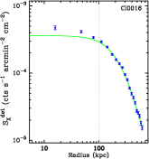
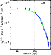
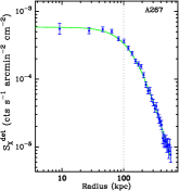
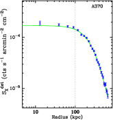
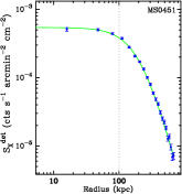
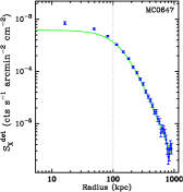
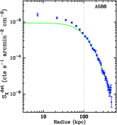
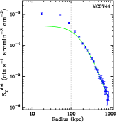
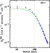
![[Uncaptioned image]](/html/astro-ph/0604039/assets/x22.png)
![[Uncaptioned image]](/html/astro-ph/0604039/assets/x23.png)
![[Uncaptioned image]](/html/astro-ph/0604039/assets/x24.png)
![[Uncaptioned image]](/html/astro-ph/0604039/assets/x25.png)
![[Uncaptioned image]](/html/astro-ph/0604039/assets/x26.png)
![[Uncaptioned image]](/html/astro-ph/0604039/assets/x27.png)
![[Uncaptioned image]](/html/astro-ph/0604039/assets/x28.png)
![[Uncaptioned image]](/html/astro-ph/0604039/assets/x29.png)
![[Uncaptioned image]](/html/astro-ph/0604039/assets/x30.png)
Cont.
![[Uncaptioned image]](/html/astro-ph/0604039/assets/x31.png)
![[Uncaptioned image]](/html/astro-ph/0604039/assets/x32.png)
![[Uncaptioned image]](/html/astro-ph/0604039/assets/x33.png)
![[Uncaptioned image]](/html/astro-ph/0604039/assets/x34.png)
![[Uncaptioned image]](/html/astro-ph/0604039/assets/x35.png)
![[Uncaptioned image]](/html/astro-ph/0604039/assets/x36.png)
![[Uncaptioned image]](/html/astro-ph/0604039/assets/x37.png)
![[Uncaptioned image]](/html/astro-ph/0604039/assets/x38.png)
![[Uncaptioned image]](/html/astro-ph/0604039/assets/x39.png)
Cont.
![[Uncaptioned image]](/html/astro-ph/0604039/assets/x40.png)
![[Uncaptioned image]](/html/astro-ph/0604039/assets/x41.png)
![[Uncaptioned image]](/html/astro-ph/0604039/assets/x42.png)
![[Uncaptioned image]](/html/astro-ph/0604039/assets/x43.png)
![[Uncaptioned image]](/html/astro-ph/0604039/assets/x44.png)
![[Uncaptioned image]](/html/astro-ph/0604039/assets/x45.png)
![[Uncaptioned image]](/html/astro-ph/0604039/assets/x46.png)
![[Uncaptioned image]](/html/astro-ph/0604039/assets/x47.png)
![[Uncaptioned image]](/html/astro-ph/0604039/assets/x48.png) \contcaption
\contcaption
Cont.
![[Uncaptioned image]](/html/astro-ph/0604039/assets/x49.png)
![[Uncaptioned image]](/html/astro-ph/0604039/assets/x50.png)
Cont.