$N$-Body Simulations of Alternative Gravity Models

Abstract

Theories in which gravity is weaker on cosmological scales have been proposed to explain the observed acceleration of the universe. The nonlinear regime in such theories is not well studied, though it is likely that observational tests of structure formation will lie in this regime. A class of alternative gravity theories may be approximated by modifying Poisson’s equation. We have run N-body simulations of a set of such models to study the nonlinear clustering of matter on 1–100 Mpc scales. We find that nonlinear gravity enhances the deviations of the power spectrum of these models from standard gravity. This occurs due to mode-coupling, so that models with an excess or deficit of large-scale power (at $k<0.2$ Mpc^-1) lead to deviations in the power spectrum at smaller scales as well (up to $k\sim 1$ Mpc^-1), even though the linear spectra match very closely on the smaller scales. This makes it easier to distinguish such models from general relativity using the three-dimensional power spectrum probed by galaxy surveys and the weak lensing power spectrum. If the potential for light deflection is modified in the same way as the potential that affects the dark matter, then weak lensing constrains deviations from gravity even more strongly.

Our simulations show that even with a modified potential, gravitational evolution is approximately universal, and our conclusions extend to models with modifications on scales of 1–20 Mpc. Based on this, the Peacock-Dodds approach can be adapted to get an analytical fit for the nonlinear power spectra of alternative gravity models, though the recent Smith et al formula is less successful. We also use a way of measuring projected power spectra from simulations that lowers the sample variance, so that fewer realizations are needed to reach a desired level of accuracy.

I Introduction

Observations of Type Ia supernovae, along with observations of the cosmic microwave background and large-scale structure, have established that the expansion of the universe is accelerating (Knop et al., 2003; Spergel et al., 2003; Riess et al., 2004). Einstein’s theory of gravity, and a cosmological model that includes dark matter, baryons and radiation, cannot explain this cosmic acceleration. The explanation may involve the existence of an exotic form of energy density, or the breakdown of general relativity (GR) on large scales. These explanations for cosmic acceleration are known as “dark energy” and “alternative gravity” approaches, respectively.

The rate at which the universe expands is predicted by the Friedmann equation $H^{2}=8\pi G\rho/3$ (for a spatially flat universe), which is derived from the Einstein equations and the metric. In order to reproduce the cosmic acceleration, we have to modify the Einstein equation:

$$R_{\mu\nu}-\frac{1}{2}Rg_{\mu\nu}=8\pi GT_{\mu\nu}.$$ (1)

The left hand side describes the curvature of spacetime due to gravity while the right hand side describes its sources. Given an observed expansion history that one wishes to describe, an alternative gravity (AG) theory will attempt to explain it via a modification of the left-hand side while a dark energy (DE) theory introduces a new term on the right-hand side that gives the desired acceleration. While one could imagine two different kinds of modifications that gave the same expansion history, they will have different effects on the growth of structure by gravitational clustering: a smooth dark energy (DE) affects the growth of structure only by changing the expansion rate, while AG affects it by direct modification of the gravitational interaction. The linear regime growth factor $G(a)$ is scale independent in DE models; an AG modification will produce a different solution, which in general is scale-dependent: $G(k,a)$ as described in Sec. II (though see Jacobs et al. (1993) for weak scale dependence in standard gravity due to the effect of inhomogeneities).

There are several potential ways of modifying GR: adding nonlinear terms in the Ricci scalar $R$ to the gravitational action, coupling $R$ to a scalar field as in Brans-Dicke gravity, having gravity operate in a higher dimensional universe on large scales as suggested by brane cosmology, introducing scalar and vector degrees of freedom and so on. The tensor-vector-scalar theory of Bekenstein (2004), the ghost condensate theory of Arkani-Hamed et al. (2004), and the five-dimensional theory of Dvali, Gabadadze, and Porrati (2000, DGP gravity) have drawn recent attention. Our interest is in the class of theories such as DGP that aim to reproduce cosmic acceleration by weakening gravity on large-scales. The theory is then likely to have testable consequences on scales probed by large-scale structure.

Lue et al. (2004a) have derived the linear growth of perturbations in DGP gravity. Further, Lue et al. (2004b) argued that generic gravity theories that obey Birkhoff’s theorem and mimic cosmic acceleration lead to the suppression of the growth of large-scale density perturbations at the level of $\sim 5\%$, similar to DGP. Predictions for the exact linear growth as a function of scale, or for scale-dependent growth in the nonlinear regime, do not yet exist in such theories.

Newton’s Law has been directly measured from millimeter to solar system scales (Adelberger et al., 2003; Hoyle et al., 2004). To constrain possible deviations from Eq. (1) on cosmological scales requires geometric information (distance measurements to objects of known redshift) and information on the growth of structure. Since the observed cosmic acceleration occurs at low redshift, observational constraints at $z<1$ are needed to learn about its origin. Geometric information at low redshift has been measured most cleanly by the measurement of the luminosity distances $d_{L}(z)$ to type Ia supernovae. Weak lensing (WL) can measure low-redshift distance information as well as the evolution of the growth factor, especially with tomography (Hu, 1999). Baryon acoustic oscillations in the power spectrum of galaxies or other probes can measure the angular diameter distance at low redshifts. The CMB (cosmic microwave background) measures geometric information (the angular diameter distance to last scattering at $z=1089$), the shape and amplitude of the primordial power spectrum, and matter/radiation content (Dodelson, 2003). Thus the CMB anchors the cosmological model at high redshift, and by comparing to it, Type Ia SN, weak lensing, baryon oscillations and galaxy cluster measurements constrain the effects of dark energy or AG. Currently, combining the CMB, SN, and large-scale structure information has led to a best-fit “standard” cosmological model (Spergel et al., 2003). This model is usually described in terms of standard gravity (GR) and dark energy; current constraints on the equation of state of dark energy are consistent with a cosmological constant, but a possible time evolving dark energy is not well constrained.

Some studies have considered the constraints on alternative gravity from existing and planned survey data (e.g. Liddle et al., 1998; Uzan and Bernardeau, 2001; Peebles, 2002; Song, 2005, 2006; Knox et al., 2005; Ishak et al., 2005; Alam and Sahni, 2005; Sawicki and Carroll, 2005; Koyama, 2006; Maartens and Majerotto, 2006). Lue et al. (2004a) and some of these authors have examined the linear regime growth factor in DGP gravity and computed its consequences for low-redshift galaxy power spectra and weak lensing observables.

In this paper we study the consequences of modifying Poisson’s equation for the growth of structure in the nonlinear regime. The model we consider for the modified Poisson equation may be regarded as an approximate description of a complete AG theory over a range of scales (though not all AG theories will be described by our approach to gravitational clustering). While our AG model is not derivable from a covariant, consistent theory of gravity, it has the merit that we can use N-body simulations to study the the full nonlinear evolution of structure. We are interested in the amplitude and scale dependence of modified growth over the range 1–100 Mpc, where cosmological observations can probe gravity effectively. An AG theory that provides an expansion history similar to the $\Lambda$CDM accelerating universe is likely to alter Newton’s Law on these scales. We note that a similar modification of the gravitational potential was considered by White and Kochanek (2001). They followed a somewhat different approach to lensing (changing the deflection angle relation while retaining the growth of structure as in standard gravity) and calculated the consequences on smaller scales (0.01–10 Mpc), as their focus was on modifications that produce flat rotation curves for galaxies without the need for dark matter.

In the linear regime, analytic calculations can explore the effects of a modification of Poisson’s equation on the growth of structure. Recent efforts in this direction were made by Shirata et al. (2005) and Sealfon et al. (2005). However observations have significant information in the small scale nonlinear regime, so it is necessary to develop predictions for this regime. Moreover, we know from perturbation theory that quasilinear effects propagate power from large to small scales, so altering gravity on large scales is likely to affect smaller structure as well. To obtain accurate nonlinear predictions, we use N-body simulations to determine the effect of modifications to Poisson’s equation in the non-linear regime on structure formation. We quantify the extent to which such a modification would be constrained by galaxy and WL surveys.

In Sec. II we describe the formalism that describes the growth of perturbations due to gravity. Sec. III contains details on our numerical simulations and predictions for three-dimensional and lensing power spectra. We describe our results in Sec. IV and conclude in Sec. V.

II Linear Regime

In Eulerian coordinates the equations that govern the behavior of mass fluctuations are given by recasting the fluid equations in expanding coordinates, or simply by conservation of stress-energy $\nabla_{\mu}T^{\mu\nu}=0$. If we linearize these equations, the resulting second order differential equation describes the growth of the fractional overdensity $\delta({\bf r},t)$, or equivalently, its Fourier transform $\tilde{\delta}({\bf k},t)$:

$$\ddot{\delta}+2H\dot{\delta} = \frac{\nabla^{2}\phi}{a^{2}},$$ (2)

$$\ddot{\tilde{\delta}}+2H\dot{\tilde{\delta}} = -\frac{k^{2}}{a^{2}}\tilde{\phi},$$ (3)

where $a(t)$ is the expansion scale factor and gives the Hubble parameter as $H(t)\equiv\dot{a}/a$. The Fourier transformed Poisson equation in comoving coordinates reads

$${\tilde{\phi}}({\bf k},t)=-\frac{3}{2}\frac{H_{0}^{2}\Omega_{\rm m0}}{a}\frac{{\tilde{\delta}}({\bf k},t)}{|{\bf k}|^{2}},$$ (4)

where $k$ is the comoving wavenumber and $\phi$ is the gravitational potential. In this work our continuous Fourier transform conventions are

$$\tilde{\delta}({\bf k}) = \int d\,^{3}{\bf r}\,\delta({\bf r})e^{i{\bf k}\cdot{\bf r}},$$ (5)

$$\delta({\bf r}) = \int\frac{d\,^{3}{\bf k}}{(2\pi)^{3}}\,\tilde{\delta}({\bf k})e^{-i{\bf k}\cdot{\bf r}}.$$ (6)

A DE modification will change Eq. (3) via the time derivatives and the Hubble parameter $H\equiv\dot{a}/a$ on the left hand side; for such a model one separates Eq. (3) by letting $\tilde{\delta}({\bf k},t)\equiv\tilde{\delta}({\bf k})G(t)$ and then solving for the growth factor $G(t)$. An AG modification will change the potential on the right-hand side via Eq. (4). We can see from this that if an AG modification is made, i.e. if $k^{2}\phi({\bf k},t)\sim\tilde{\delta}({\bf k},t)f({\bf k},t)$ for some non-trivial $f({\bf k},t)$, Eq. (3) will no longer be separable, and hence the growth factor will become scale dependent, i.e. one must allow $\tilde{\delta}({\bf k},t)\equiv\tilde{\delta}({\bf k})G({\bf k},t)$. Eq. (3) then becomes

$$\ddot{G}({\bf k},t)+2H\dot{G}({\bf k},t)=\frac{3}{2}\frac{H_{0}^{2}\Omega_{\rm m0}}{a^{3}}G({\bf k},t)f({\bf k},t).$$ (7)

If $f({\bf k},t)\rightarrow 1$ then $G({\bf k},t)\rightarrow G(t)$ as in standard gravity. We note that a purely time-dependent modification $f(t)$ (such as a time-dependent Newton’s constant), can be accommodated without a scale-dependent growth factor.

II.1 Modified Poisson Equation

Figure 1: Ratios of linear theory alternative gravity (AG) power spectra to standard gravity at $z=0$, for different parameterizations of Eq. (9). The dotted lines are the matter power spectrum ratios $P_{\delta,{\rm alt}}/P_{\delta,{\rm std}}=(G_{\rm alt}(k,t)/G_{\rm std}(t))^{2}$. The dashed lines are the ratios of the velocity power spectra $P_{v,{\rm alt}}/P_{v,{\rm std}}=(\dot{G}_{\rm alt}(k,t)/\dot{G}_{\rm std}(t))^{2}$. The expansion history is fixed to be the same as for a $\Lambda$CDM universe.

A theory of gravity that makes gravity weaker or stronger over a range of length scales can be approximated by modifying Poisson’s equation. Sealfon et al. (2005) investigated the effect of a Yukawa-type (adding an exponential term) and power-law modifications to the Poisson equation, solving for the scale-dependent growth factor $G({\bf k},t)$ under the assumption that the modification was a small perturbation to the Newtonian potential. Shirata et al. (2005) followed by obtaining $G({\bf k},t)$ for a Yukawa modification of arbitrary strength. They adopted the Peacock-Dodds (PD) prescription (Peacock and Dodds, 1996) — an approach we check with our simulations — to obtain the non-linear matter power spectrum from the linear solution. With a prescription for galaxy biasing, this enabled them to predict galaxy power spectra, which they used with their AG model to constrain model SDSS galaxy power spectrum measurements (Tegmark et al., 2004).

Both Shirata et al. (2005) and Sealfon et al. (2005) consider the real-space potential

$$\phi_{\rm alt}({\bf r})=-G\int d\,^{3}{\bf r}^{\prime}\frac{\rho({\bf r}^{\prime})}{|{\bf r}-{\bf r}^{\prime}|}\left[1+\alpha\left(1-e^{-\frac{|{\bf r}-{\bf r}^{\prime}|}{r_{\rm s}}}\right)\right].$$ (8)

In Fourier space, this becomes

$$\widetilde{\nabla^{2}\phi}_{\rm alt}({\bf k})=\frac{3}{2}\frac{H_{0}^{2}\Omega_{\rm m0}}{a}\delta({\bf k})\left[1+\alpha\frac{1}{1+(|{\bf k}|r_{\rm s}/a)^{2}}\right].$$ (9)

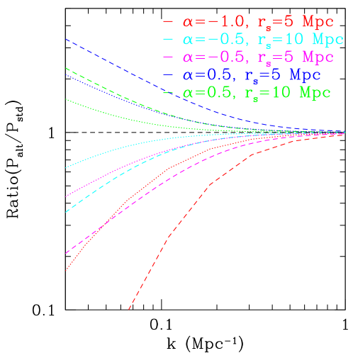
Note that this will result in a scale dependent growth factor when plugged into Eq. (2) above. In Fig. 1, we can see the effect of this modification on the linear theory power spectrum; there we have plotted the ratio of the AG matter and velocity linear power spectra to the corresponding standard linear spectrum at redshift $z=0$ for a few different parameterizations of Eq. (9). Throughout this work, we fix the background expansion to be the same as $\Lambda$CDM, i.e. we take

$$H^{2}(a)=H_{0}^{2}(\Omega_{\rm m0}a^{-3}+\Omega_{\rm\Lambda 0}).$$ (10)

In this study we do not allow the acceleration to vary with $\alpha$ or $r_{s}$; we let it be fixed solely by $\Lambda$, because an AG theory would need to predict an accelerating expansion not too different from that given by $\Lambda$CDM in order to fit the supernova data. For Fig. 1 and our simulations we take $\Omega_{\rm m0}=0.3$, and $\Omega_{\rm\Lambda 0}=0.7$.

The matter power spectrum $P_{\delta}(k)\propto G^{2}(k,t)$, while the velocity power spectrum $P_{v}(k)\propto\dot{G}^{2}(k,t)$, so the ratios of the growth factors give us the ratios of the linear spectra starting from the same initial spectrum. We solve for the growth factor using Eq. (7). The velocity power spectra show a more pronounced difference than the matter spectra (a factor of 2-5 larger deviation at $k\approx 0.05$ Mpc^-1). It may be worth exploring the measurement of large-scale peculiar velocities via the kinetic SZ effect or distance measurements on galaxies to test gravity.

On large and small scales, we get the limiting behavior

$$r\gg r_{\rm s},\ \ \phi_{\rm alt} \rightarrow (1+\alpha)\phi_{\rm newton},$$ (11)

$$r\ll r_{\rm s},\ \ \phi_{\rm alt} \rightarrow \phi_{\rm newton}.$$ (12)

So for positive $\alpha$, the alternative gravity potential is stronger than Newtonian gravity on large scales and unchanged on small scales. Shirata et al. take $r_{\rm s}$ to be a fixed physical length, that is, in comoving units it changes with redshift; consequently, at early times when $a\ll 1$, $r_{s}$ becomes very large. At our simulation starting point of $z=50$, $r_{s}$ is much larger than the boxsize, and so the linear spectra are virtually identical. Hence both the alternative and the standard gravity simulations start from the same initial conditions. We examine the effect of the initial conditions further in Sec. IV.

We note that this modification cannot extend to arbitrarily large scales or early times. We regard it as an approximate description of gravity on length scales well below the horizon at low redshifts.

III Numerical Simulations

While Eq. (2) is useful for describing linear-regime density fluctuations on large scales, if we want a more complete description we have to turn to numerical simulations. An N-body code simulates the evolution of structure by evolving a large number of particles interacting by gravity. These are evolved from early times ($z\gg 1$) up to the present, with particle positions and velocities outputted at regular intervals.

An efficient N-Body solver must compute the forces on a large number of particles simultaneously so that the equations of motion can be integrated forward in time. We use a basic particle-mesh (PM) solver for this purpose, which interpolates the particles onto a grid and then computes the potential via Fourier transform. More advanced techniques (e.g. P³M and tree codes) are available, which provide larger dynamic range in exchange for greater complexity and computation time. We use PM simulations to simulate modified gravity in the quasilinear to moderately nonlinear regime where observations can test models without needing to consider astrophysical/baryonic effects. Due to the lower CPU costs of PM simulations, we were able to run a large number of realizations to reduce sample variance on the power spectra, which would have been prohibitive with the other methods. Our code is based on the PM code of Klypin and Holtzman (1997), which was designed and tested for DM simulations (Klypin et al., 1993, 1995), and kindly made available by A. Klypin. We set up the initial conditions by displacing particles from a regular grid using a realization of the linear power spectrum.

III.1 Discrete Poisson Equation

In the PM simulation, the equations of motion are discretized on a grid, starting with the Poisson equation. Since we modify this equation for the AG simulations, we give the explicit formulae here. We define the second derivative operator in 1-D as

$$\nabla^{2}\phi_{i}\approx\phi_{i+1}+\phi_{i-1}-2\phi_{i}.$$

We define the unnormalized discrete Fourier transform as

$$\tilde{\phi}_{k} = \sum_{r=0}^{N-1}\phi_{r}e^{i2\pi rk/N},$$

$$\phi_{r} = \sum_{k=0}^{N-1}\tilde{\phi}_{k}e^{-i2\pi rk/N}.$$

Combining the previous two equations leads to the discrete Fourier space expression

$$\widetilde{\left[\nabla^{2}\phi\right]}_{k}=\tilde{\phi}_{k}\times 2\left[\cos{\frac{2\pi k}{N}}-1\right]$$ (13)

So the 3-D discrete Poisson equation for standard gravity in Fourier space reads

$$\tilde{\phi}_{k}=\frac{3}{2}\frac{H_{0}^{2}\Omega_{\rm m0}}{a}\frac{\tilde{\delta}_{k}}{G_{k}},$$ (14)

where

$$G_{k}\equiv 2\left[\cos{\frac{2\pi k_{x}}{N}}+\cos{\frac{2\pi k_{y}}{N}}+\cos{\frac{2\pi k_{z}}{N}}-3\right].$$ (15)

Figure 2: Dimensionless 3D power ($\Delta^{2}_{\delta}(k)=k^{3}P_{\delta}(k)/2\pi^{2}$, left panel) and convergence power ($\Delta^{2}_{\kappa}(\ell)=\ell^{2}P_{\kappa}(\ell)/2\pi$, right panel) from N-body simulation with a standard (Newtonian) gravity model. Also shown are the Smith et al. (solid black line) and Peacock-Dodds (solid red line) fitting formulae. The points with error bars are an average over 8 realizations. Three sets of simulations are shown with varying resolution due to differences in the total number of particles; the total number of grid points in each set is $N_{\rm g}=8N_{\rm p}$.

Figure 3: Dimensionless 3D power and convergence power spectra from simulation, shown together with the Smith and PD fitting formulae as in Fig. 2. Three different boxsizes are shown: $100h^{-1}$, $200h^{-1}$, and $500h^{-1}$ Mpc.

III.2 Particle-Mesh Simulation Parameters

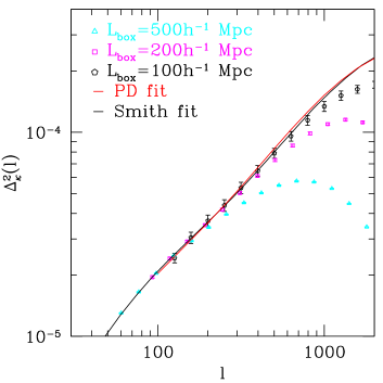
The parameters which determine the dynamic range of a PM simulation are the boxsize $L_{\rm box}$, the number of particles $N_{\rm p}$, and the Fourier grid size $N_{\rm g}$. The grid spacing should be smaller than the mean particle spacing to preserve the small scale resolution; a common choice which we adopt is to take $N_{\rm g}=8N_{\rm p}$, i.e. twice the number of particles per dimension. $L_{\rm box}$ must be large enough so that we have enough power in the linear regime to get accurate power spectra, however increasing $L_{\rm box}$ decreases one’s ability to resolve small-scale structure for fixed $N_{\rm p}$. Our computational resources fixed $N_{\rm g}=256^{3}$ and $N_{\rm p}=128^{3}$; we chose $L_{\rm box}=100h^{-1}\simeq 140$ Mpc for our boxsize. The wavenumber corresponding to $L_{\rm box}$ is $k_{\rm min}\approx 0.04$ Mpc^-1; the comoving distance to the sources is $\chi(z=1)\approx 3.3$ Gpc, so the angular wavenumber is $\ell_{\rm min}=k_{\rm min}\chi\approx 145$, corresponding to a field of view $\sim 2.5^{\circ}$ on a side.

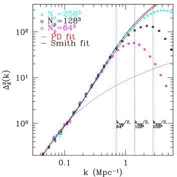
To check our results in the non-linear regime, and to insure that we chose $L_{\rm box}$ large enough, we tested our prediction for the 3D power for standard gravity against the Smith et al. (2003) fitting formula. We find in Fig. 2 that for our runs of $N_{\rm p}=128^{3}$ particles on a $N_{\rm g}=256^{3}$ grid, our results are limited by resolution at physical scales of about 1.0 Mpc, and angular scales of $\ell\approx 1000$. The power spectrum $\Delta^{2}_{\delta}(k)$ in Fig. (2) is identical to the linear theory prediction on large scales; we have about a decade of power in the linear regime at $z=0$. With our sources at $z_{s}=1$, the weak lensing weight function $W(\chi)$ in Eq. (19) peaks at $z\approx 0.4$ where the linear regime extends to smaller scales. So we can be confident that for purposes of measuring the lensing power spectrum our choice of $L_{\rm box}=100h^{-1}$ Mpc is large enough.

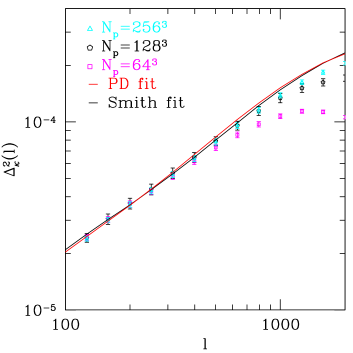
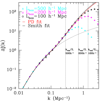
Fig. 2 and Fig. 3 show how the resolution limit behaves as we change the number of particles or the boxsize in the simulation. We note that since we are not including direct particle-particle effects (as in P³M-type codes) we don’t need to be concerned with explicit force softening, and that the shot-noise contribution is very small on the scales that we resolve.

The particle mass in our simulation $m_{\rm p}$ is given by

$$m_{\rm p}=\Omega_{\rm m0}\ \rho_{{\rm cr},0}\ \left(\frac{L_{\rm box}^{3}}{N_{\rm p}}\right)$$ (16)

For our simulations with $N_{\rm p}=128^{3}$ and $L_{\rm box}=100h^{-1}$ Mpc, we get $m_{\rm p}=1.1\times 10^{10}$ $M_{\odot}$.

We ran all of our simulations in a ${\rm\Lambda CDM}$ background cosmology. They were started at redshift $z=50$. We used $\sigma_{8}=1.0$, $H_{0}=70$, $\Omega_{\Lambda}=0.7$, and $\Omega_{m}=0.3$ as our cosmological parameters. We ran 8 realizations for our runs with standard gravity and for each of the alternative gravity models.

III.3 Convergence Power Spectrum

The output of N-Body simulations has been used to make model shear and convergence maps of cosmological weak lensing (Jain et al., 2000; White and Hu, 2000). Unlike the angular power spectrum of the CMB, which can be computed analytically, weak lensing involves the deflection of light by large scale structure at low redshift, which has already undergone significant nonlinear collapse, so model WL maps and power spectra must be computed numerically.

In the standard multiple lens plane algorithm, the convergence and shear maps are computed by filling the light cone from the observer to the source galaxies with matter from N-body simulation outputs. Starting at the source redshift, one can output three orthogonal 2D-projections (slices) of the density field at length intervals equal to the box size. By picking a projection at each redshift and randomly translating the boxes, we tile approximately uncorrelated mass distributions along a light cone for each realization. The box size at the source redshift determines the field of view simulated.

Figure 4: Comparison of the dimensionless convergence power using our Limber approximation method (red triangles) and the standard multiple lens plane method (blue squares), each averaged over 8 realizations. Computing $P_{\kappa}$ in the standard method (using Eq. (22)) uses only the 2D modes of the density field at each redshift slice. We included the full 3D modes by using the Limber equation for $P_{\kappa}$ (Eq. (24)). The scatter is significantly smaller, as shown by the error bars on the red symbols. The black curve is computed using the Peacock and Dodds (1996) 3D power spectrum.

Following Bartelmann and Schneider (2001), in the thin-lens approximation for a flat universe, the convergence $\kappa(\theta)$ is a sum over slices of the transverse gradient of the potential at comoving distances $\chi_{i}$ (with sources fixed at $\chi_{s}$):

$$\kappa({\bm{\theta}})=\frac{1}{c^{2}}\sum_{i}L_{\rm box}W(\chi_{i},\chi_{s})\nabla^{2}_{\bm{\theta}}\phi(\chi_{i}{\bm{\theta}},\chi_{i}).$$ (17)

In standard general relativity, we can use the Poisson equation, the real-space version of Eq. (4), to obtain

$$\kappa_{\rm std}({\bm{\theta}})=\frac{3H_{0}^{2}\Omega_{\rm m0}}{2c^{2}}\sum_{i}L_{\rm box}W(\chi_{i},\chi_{s})\frac{\delta^{\rm 2D}_{i}(\chi_{i}\theta)}{a(\chi_{i})},$$ (18)

where $L_{\rm box}$ is the tile boxsize, and

$$W(\chi_{i},\chi_{s})\equiv\frac{\chi_{i}(\chi_{s}-\chi_{i})}{\chi_{s}}$$ (19)

is the weak lensing weight function. If the photons feel the same modified potential as the dark matter, then we must use a modified Poisson equation such as Eq. (8) instead; note that this is not true in some theories, e.g. in the fifth force-type modification of Nusser et al. (2005). The converse has also been considered: White and Kochanek (2001) constrained the parameters of a model where the potential affecting photons was modified, but structure was assumed to have formed as in GR. Since we are interested in scales ($\ell\geq 100$), we use the flat-sky approximation and define the 2D Fourier transform as

$$\tilde{\kappa}({\bm{\ell}}) = \int d\,^{2}{\bm{\theta}}\,\kappa({\bm{\theta}})e^{i{\bm{\ell}}\cdot{\bm{\theta}}},$$ (20)

$$\kappa({\bm{\theta}}) = \int\frac{d\,^{2}{\bm{\ell}}}{(2\pi)^{2}}\,\tilde{\kappa}({\bm{\ell}})e^{-i{\bm{\ell}}\cdot{\bm{\theta}}}.$$ (21)

Assuming the mass distribution in different redshift slices is uncorrelated, the convergence power spectrum in this approximation is a sum over the 2D power spectra of the projected densities:

$$\langle|\tilde{\kappa}(\ell)|^{2}\rangle\propto\sum_{i}\frac{W^{2}(\chi_{i},\chi_{s})}{a^{2}(\chi_{i})}f^{2}\left(k=\frac{\ell}{\chi_{i}},a(\chi_{i})\right)\langle|\tilde{\delta}_{i}^{\rm 2D}(\ell)|^{2}\rangle.$$ (22)

Here we have included the function $f({\bf k},a)$, introduced in Eq. (7), that describes the modification of gravity in the Poisson equation; for the model we consider in this paper (i.e. Eq. (9)),

$$f({\bf k},a)=1+\alpha\frac{1}{1+(|{\bf k}|r_{\rm s}/a)^{2}}.$$ (23)

We can already see that if an AG modification changes the potential felt by dark matter and photons in the same way, then WL results can provide a stronger constraint on AG. In Eq. (22), the modification will affect the two-point function $\langle|\tilde{\kappa}(\ell)|^{2}\rangle$ twice: once via the modified growth of structure from the $\langle|\tilde{\delta}_{i}^{\rm 2D}(\ell)|^{2}\rangle$ term, and once via the $f^{2}(k,a)$ term that comes directly from the modification of the potential. We show in Sec. IV that for our model, these effects of AG combine to produce a dramatic effect.

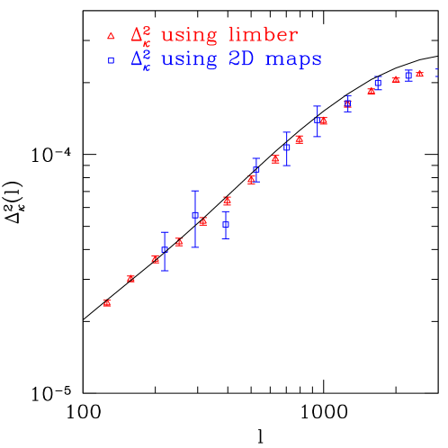
Computing the convergence power spectrum from Eq. (22) uses only the 2D modes of the density field at each redshift slice; a large part of the information in each simulation box is lost by the projection. In order to reduce the scatter in the simulations, we included the full 3D modes in our computation of $P_{\kappa}(\ell)$ from our data. We accomplished this by using the Limber approximation to compute $P_{\kappa}$ directly as an integral over the 3D matter power spectrum $P_{\delta}$:

$$P_{\kappa}(\ell)=\frac{9H_{0}^{4}\Omega_{\rm m0}^{2}}{4c^{4}}\Delta\chi\sum_{i}\frac{W^{2}(\chi_{i})}{\chi_{i}^{2}a^{2}(\chi_{i})}f^{2}\left(k=\frac{\ell}{\chi_{i}},a(\chi_{i})\right)P_{\delta}\left(k=\frac{\ell}{\chi_{i}},\chi_{i}\right).$$ (24)

Traditionally, Eq. (24) is used to compute $P_{\kappa}(\ell)$ when one has an estimate of $P_{\delta}(k)$ from the halo model or other fitting formula. Instead we use Eq. (24) with $P_{\delta}$ measured from the PM simulations at redshifts $z_{i}$. This results in a significant gain in our signal-to-noise for $P_{\kappa}$ as shown in Fig. 4: the error bars in the standard method based on measuring $P_{\kappa}$ from $\kappa$ maps are significantly larger than in our method.

Figure 5: Dimensionless 3D power and convergence power spectra from simulation. The colored pentagons are simulation data produced using a 400h^-1 Mpc box, the squares have a 200h^-1 Mpc box, and the triangles have 100h^-1 Mpc (which we use in the main portion of our simulations). The simulations are consistent with each other up to their resolution limit, regardless of whether or not $r_{s}$ is initially outside the box.

For each realization we obtain the power spectrum in $100h^{-1}$ Mpc boxes tiled along the line of sight. Using the discrete version of Equation (24) we get $P_{\kappa}(\ell)$ for each realization from $P_{\delta}(k)$ binned in spherical shells in wavenumber $k$; the bins we need at each redshift are given by $k=\ell/\chi_{i}$. Eight realizations give us our estimate of the scatter in our results. We take our results to be valid up to wavenumber $k\approx 1$ Mpc^-1, which is about $k_{\rm nyq}/2$; for $P_{\kappa}$ this corresponds to $\ell\approx 1000$. Additionally, we have checked the validity of our modified gravity simulations for larger boxsizes. Since at the start of our simulation, the comoving scale $r_{s}(z=50)\approx 250$ Mpc is larger than $L_{\rm box}=100$h^-1 Mpc, but at $z=0$, $r_{s}\ll L_{\rm box}$, we needed to insure that no numerical artifacts are produced when $r_{s}$ crosses the box scale. In Fig. 5, we find that this is indeed the case.

Figure 6: Dimensionless 3D power ($\Delta^{2}_{\delta}(k)=k^{3}P(k)/2\pi^{2}$) and convergence power ($\Delta^{2}_{\kappa}(\ell)=\ell^{2}P_{\kappa}(\ell)/2\pi$) for standard and alternative gravity models. The black curves for standard gravity are computed using the Peacock and Dodds (1996) fitting formula for the nonlinear 3D power, and using it in the Limber integral for $P_{\kappa}$. The dotted curves are predictions from linear theory. The solid curves are our analytic fits for the nonlinear spectra of modified gravity models (as indicated by the legends), while the symbols show simulation measurements. The two subpanels for $\Delta^{2}_{\kappa}$ illustrate two choices for how WL power spectra are affected by a modified potential: the curves in the left subpanel are computed assuming a GR deflection law, i.e. setting $f^{2}=1$ in Eq. (24), whereas those on the right are computed with a modified potential for photons. The error bars on the solid curves in the right panels show the expected statistical errors from a future lensing survey (see text in Section 4 for details).

Figure 7: Ratio plots of dimensionless 3D power ($\Delta^{2}_{\delta}(k)=k^{3}P(k)/2\pi^{2}$) and convergence power ($\Delta^{2}_{\kappa}(\ell)=\ell^{2}P_{\kappa}(\ell)/2\pi$). The solid curves show the ratio of the Peacock-Dodds prediction for AG with standard gravity. The dotted curves are the linear theory ratios. We divided our AG simulation power spectra by the corresponding points from the standard gravity simulation to obtain the points. As in Fig. 6, the left $P_{\kappa}$ subpanel shows the WL result for the GR deflection law, while the right subpanel shows that the deviation of AG from the standard gravity result is substantially enhanced if the deflection law is modified along with the growth of structure. The error bars on the horizontal line in the right panels show the expected statistical errors from future lensing surveys (see text for details).

IV Simulation Results

We have run ensembles of simulations using standard gravity and the AG potential given by Eqs. (8, 9) with five different sets of parameters: $\alpha=0.5,r_{\rm s}=5$ Mpc; $\alpha=-0.5,r_{\rm s}=5$ Mpc; $\alpha=0.5,r_{\rm s}=10$ Mpc; and $\alpha=-0.5,r_{\rm s}=10$ Mpc. These sets of parameters are within the $2\sigma$ range of constraints set by Shirata et al. using SDSS data; the last two models given have the smallest deviation from standard gravity, for these models the linear spectrum differs by 20% at $k=0.05$ Mpc^-1. We also consider a model that has significantly less power on large scales: $\alpha=-1.0,r_{s}=5$ Mpc.

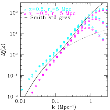
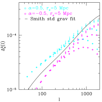
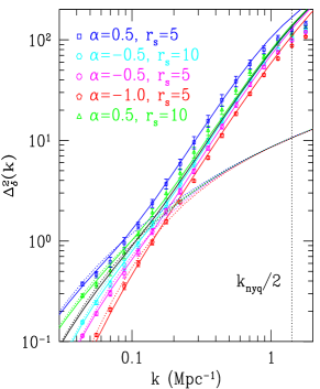
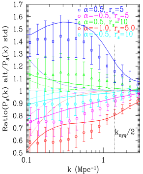
The left panel of Fig. 6 shows the 3D power for standard gravity and the five AG models, while the left panel of Fig. 7 shows them as ratios to standard gravity. There is a statistically significant difference between the models at the smallest scales resolved by our simulations, where the general trend is that models with larger $|\alpha|$ and smaller $r_{s}$ are more different from standard gravity. The overall shape of the linear and nonlinear AG spectra remains similar to the shape of the standard gravity spectra; as expected, the positive $\alpha$ models have excess power on large scales, while the models with negative $\alpha$ have less large-scale power compared to standard gravity. The nonlinear scale of each of the models is around $k=0.1$–0.2 Mpc^-1, similar to standard gravity; on scales smaller than this, the linear spectra asymptote to the standard gravity linear curve. However, the 3D nonlinear spectra show clearly that changing gravity on large scales propagates into the nonlinear regime: in the nonlinear region $k=0.5$–1.0 Mpc^-1, where the linear spectra are within a few percent of standard gravity, the nonlinear 3D spectra differ by 10% or more.

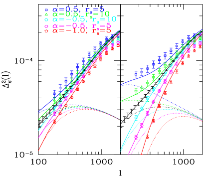
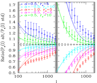
The $P_{\kappa}$ plots in Figs. 6,7 are split up into two subpanels: in the left subpanel, photons are not affected by the modification of the potential (but the growth of structure is still altered), corresponding to setting $f^{2}=1$ in Eq. (24), while in the right panel photons feel the modified potential. Each $P_{\kappa}$ is given by the limber integral over the corresponding $P_{\delta}$ in the left panel, the difference is only whether the $f^{2}$ term in Eq. (24) is included. If light deflection and structure formation are both affected by the modified potential, then the difference between the $P_{\kappa}$ subpanels in Figs. 6,7 shows that an AG model would be much more easily ruled out. Because the modified potential for photons and the modified growth of structure can reinforce each other, WL statistics potentially have more power to constrain AG theories than large-scale structure observations (such as the galaxy power spectrum) do: in the left panel of Fig. 7, we see that the cyan and green models ($|\alpha|=0.5$, $r_{s}=10$ Mpc) are perhaps just barely detectable using the power spectrum; but if light deflection as well as large-scale structure is modified, these models are easily ruled out.

For $P_{\kappa}$ as well the differences from standard gravity extend to smaller angular scales; at our resolution limit of $\ell\sim 1000$, there are still observable differences at the level of several standard deviations for our fiducial survey. The error bars on the black lines in each of the right panels are the statistical errors from a hypothetical lensing survey with $f_{\rm sky}=0.1$ and $n_{\rm gal}=40$ arcmin^-2. The general trends are the same as for $P_{\delta}$: the models with larger $|\alpha|$ and smaller $r_{s}$ exhibit larger deviations from standard gravity, and the linear and nonlinear spectra are more different on large angular scales. As is evident from Fig. 6, while the linear $P_{\kappa}$ asymptotes to the the standard gravity result on small scales, in the observable regime ($\ell>100$), $P_{\kappa}$ has nonlinear contributions. Here we have not performed a full parameter analysis that would involve CMB priors and variations of all relevant parameters.

Figure 8: Comparing the effect of changing the initial conditions to changing the potential. The ICs at $z=50$ are on the left, and the $z=0$ outputs are on the right. The cyan and magenta points are simulations that have a modified initial spectrum shape but are evolved with the standard gravity potential, while the red and blue points are evolved using the AG potential with the correct initial spectrum (as in the rest of the paper). The two pairs of points for each model (blue and cyan points, and the red and magenta points), are within errors of each other at the end of the simulation (the $z=0$ right panel). Hence there is an approximate degeneracy between the shape of the initial power spectrum and the shape of the potential during its evolution under gravity.

IV.1 Analytical Approximations

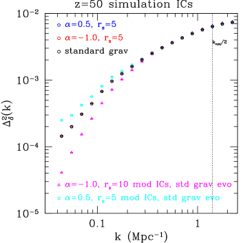
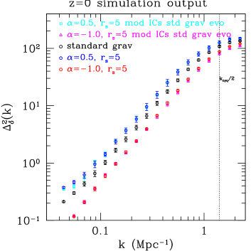
From the power spectra in Fig. 6 and Fig. 7, one cannot tell whether the observed differences on small scales at late times are a result of the changed non-linear evolution in the AG models, or whether the structure formed under the influence of normal gravity and merely started from different initial conditions.

To answer this question we ran simulations whose initial conditions had the same shape as the late-time AG linear power spectrum, but were evolved using the standard gravity potential. The results, shown in Fig. 8, are striking: the 3D power spectra of simulations, which had the $z=0$ linear shape of the AG model at the initial time, came out the same as the regular AG runs. Recall that since $r_{s}$ is a fixed physical length scale in the AG model, at the start of the simulation at $z=50$, it is $250-500$Mpc in comoving coordinates. This is larger than the simulation box size of $100h^{-1}$ Mpc. So we would expect the AG power spectrum at $z=50$ to be identical to that of standard gravity.

The plots in Fig. 8 show a kind of universality in cold dark matter structure formation: the way non-linear structures form is not uniquely determined by specifying the detailed shape of the potential. Our simulations show that the DM power spectrum by itself cannot distinguish between changing the shape of the initial power spectrum and changing the shape of the gravitational potential.

Figure 9: Dimensionless power for negative and positive $\alpha$ models at different redshift, compared to the Smith et al. (2003) (blue, dashed) and Peacock and Dodds (1996) (red, solid) fitting formulae. The $z=0$ outputs have been translated by a factor of 4 in the $y$-direction for legibility. For negative $\alpha$, PD fits better than Smith, while for positive $\alpha$, the simulation points lie between the two predictions.

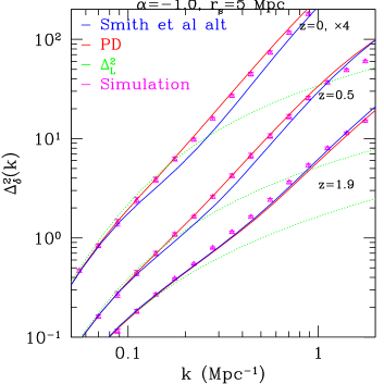
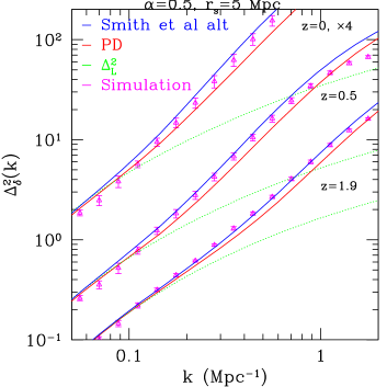
This is further revealed by testing the power spectra measured in simulations against analytical fitting functions that have been calibrated for standard gravity. The Peacock-Dodds (PD) formula (Peacock and Dodds, 1996), using a mapping of length scales between the linear and nonlinear regime, gives the dimensionless nonlinear 3D power spectrum $\Delta^{2}_{\delta}$ as a function of the dimensionless linear power $\Delta^{2}_{\rm\delta,L}$ to around 10% accuracy (when compared to simulations). Shirata et al. (2005) use the PD formula to extend their results to non-linear scales.

We have tested the PD formula with AG simulations by replacing the standard gravity linear power spectrum in the formula with the linear spectrum from the AG model. The results for $P_{\delta}$ are shown in the left panel of Fig. 6, in which the dashed lines are produced using the Peacock-Dodds formula. The right panel shows $P_{\kappa}$ fits generated by integrating the 3D power along the line of sight using the Limber approximation. The fits in Fig. 6 are accurate at about the 10% level, with the accuracy apparently better for models closer to standard gravity. From the ratio plots in Fig. 7, we also see that the positive $\alpha$ model (more large scale power) does worse.

The fitting formula of Smith et al. performs the same task as the PD formula in that, given a wavenumber $k$ and redshift $z$, it provides an estimate of the non-linear power spectrum $\Delta^{2}_{\delta}(k,z)$. The Smith formula is inspired by the halo model: it breaks up the non-linear power into two pieces, a quasi-linear term and a one-halo like term. We adapted the Smith formula for use with alternative gravity by using the AG linear spectrum, but we see in Fig. 9 that PD is a much better fit to the data for negative $\alpha$ (for the positive-$\alpha$ model that we have tested, the Smith and PD fits are comparable at low redshift). This may be due to the use of two separate terms in the Smith formula, one of which is calibrated on the basis of the shapes of CDM halos in standard gravity. It was designed and tested for simulations with scale-free initial spectra or CDM initial conditions, but not for initial spectra with a very different shape, such as those produced by a scale-dependent growth factor, initial conditions with a shape like those in Fig. 8.

To summarize, our results suggest that the nonlinear power spectrum in alternative gravity models is captured completely by the change in the linear growth factor. This result is consistent with the approach used in the PD fitting function. A similar result is shown in the recent study of Linder and White (2005), who found that nonlinear spectra for a class of dark energy models can be accurately described by appropriate choice of length and time scales. We must emphasize, however, that our results are only valid for a certain range of scales. We can estimate over what range our results should be valid by examining what happens to the comoving scale $r_{s}$ and the nonlinear scale as the simulation progresses. The comoving wavenumber corresponding to $r_{s}$ is defined by $k_{s}(z)=2\pi/((1+z)r_{s})$. For a $r_{s}=5$ Mpc model, Fig. 10 shows how the wavenumber $k_{s}$ ranges from approximately 1.3 Mpc^-1 at the present to 0.16 Mpc^-1 at $z=6.78$. Inspection also reveals that the nonlinear wavenumber $k_{\rm nl}$ (the scale where the linear and nonlinear spectra begin to diverge) ranges from approximately $k_{\rm nl}=0.2$ Mpc^-1 at the present to $k_{\rm nl}=0.5$ Mpc^-1 at $z=6.78$ for the $\alpha=-1$, $r_{s}=5$ Mpc model. So we see that $r_{s}$ actually starts out larger than $r_{\rm nl}$, but ends up well inside the nonlinear scale as time goes by; the redshift where they coincide depends on the values of $r_{s}$ and alpha chosen, for $\alpha=-1$, $r_{s}=5$ Mpc one can see that it occurs at about $z\approx 3.2$, whereas for the $\alpha=0.5$, $r_{s}=10$ Mpc model, the scales cross later at a redshift of around $z\approx 1.9$. As long as the boxsize and resolution of our simulations can adequately capture the dynamics of $r_{s}$ and $r_{\rm nl}$ over a range of redshifts, i.e. for any model where the nonlinear scale and $r_{s}$ cross well before redshift $z=0$, the conclusions we reach from our simulation should be valid; we estimate that this would be true for a range of $r_{s}$ at least from about 1 Mpc to 20 Mpc.

Figure 10: Dimensionless 3D power spectrum ($\Delta^{2}_{\delta}(k,z)=k^{3}P(k,z)/2\pi^{2}$) as a function of wavenumber and redshift for two different modified gravity models. The solid lines are the linear spectra while the points and error bars are the average of eight realizations from simulation; the vertical long-dashed lines indicate the value of $k_{s}(z)=2\pi a(z)/r_{s}$, which is the comoving wavenumber corresponding to the physical scale $r_{s}$. The nonlinear scale $k_{\rm nl}(z)$ can be read off the graph by observing where the linear and nonlinear power spectra begin to diverge. We can see that in each model, $k_{s}<k_{\rm nl}$ initially, but at $z=0$, $k_{s}>k_{\rm nl}$ in each case.

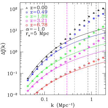
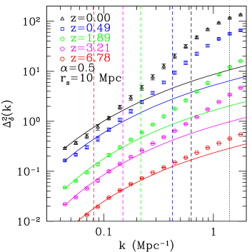
It is interesting that quasilinear perturbation theory (Jain and Bertschinger, 1994; Bernardeau et al., 2002) would have suggested some departures from this universality: equations for the second order density and velocity fields contain the linear fields as well as the $\nabla\phi$ term in the Euler equation. So the dependence of the second order terms on the scale dependent function $f(k,t)$ introduced in Eq. (7) would not be completely determined by the linear solution. Our results show that this quasilinear departure is likely very small. Generally speaking, the halo model description, assuming it describes alternative gravity models, is consistent with universality: halo bias, the linear spectrum and halo mass function depend only on the linear growth and initial power spectrum. Since the small scales where halo structure may play a role are not well probed by our simulations, it is not surprising that we find an approximate universality in the nonlinear power spectrum. The PD formula gives results close to the halo model for $\Lambda$CDM (Smith et al., 2003).

V Discussion

We have performed N-body simulations of large scale structure formation with a modified Newtonian potential in a $\Lambda$CDM background. This is intended to approximate alternative gravity theories that are designed to match the observed acceleration of the universe. We focus on the quasilinear and non-linear regime of clustering at low redshift. Our simulations resolve the 3D power spectrum of matter on scales of $k\approx 0.05$–1.0 Mpc^-1. We used the 3D simulations to compute the weak lensing power spectrum over angular wavenumbers $\ell\approx 100$–1000. We used a technique for this that reduces the scatter in measurements from simulations (described in Section 3.3). The range of scales we studied is expected to be observable with high accuracy with planned surveys. The nonlinear modification of the power spectra ranges from $10\%$ effects in the quasilinear regime to an order of magnitude at the small scale end. While the accuracy of our simulated spectra is typically $10\%$ over this range, the relative accuracy for predictions of different gravity models is significantly better.

We find that nonlinear effects propagate the difference between the power spectra to scales where the linear spectra are nearly identical. This is the expected effect of mode coupling in nonlinear gravitational evolution (Jain and Bertschinger, 1994). The result is that at scales of $k\approx 0.5$ Mpc^-1, the modified gravity power spectra differ by over 10$\%$, while the linear spectra are within 5$\%$. Similar differences are seen in the weak lensing spectra at $\ell\approx 500$, and if the potential for photons is modified in a similar way as the potential for matter, the effects reinforce each other and the differences in the weak lensing spectra are much larger. These scales are of great interest because the observational errors are expected to be small and theoretical interpretation can be made without modeling of non-gravitational effects (at least for the lensing spectra). We compare the differences between models to the expected statistical errors from a wide area lensing survey to show that it should be possible to directly constrain the parameters of an alternative gravity scenario. Models within the 2-$\sigma$ limits of current galaxy surveys would be easily distinguished by future lensing measurements. A detailed study of this is left for future work.

Our results are consistent with a universality in nonlinear gravity, which makes the nonlinear power spectrum a function only of the initial (Gaussian) conditions and linear growth, for modifications on length scales for which there are likely to be precise observations in the near future. We find that the lensing and 3D power spectra cannot distinguish between simulations which were started with appropriately modified initial conditions and evolved with standard gravity, and those which were evolved with a modified gravitational potential. This means that for observationally accessible scales, there is a degeneracy between the shape of the potential used to evolve the simulation and the shape of the initial conditions. For simple modified gravity models, it means that another constraint on the primordial power spectrum (such as the CMB), or measurements at multiple redshifts, must be used to test for modified gravity. It may also be that the structure of dark matter halos, not well probed by our simulations, are different for AG models. This is an interesting topic for future work with higher resolution simulations. The skewness or bispectrum may also help distinguish alternative gravity models, as suggested by Bernardeau (2004) and Sealfon et al. (2005), since its dependence on the scale dependent function $f(k,t)$ in Eq. (7) is different.

We tested analytical approximations to the nonlinear spectra for modified gravity models. We found that while the Peacock-Dodds fitting formula was accurate to 10–20% in comparison to the simulated spectra, its relative accuracy between different models is significantly better and within the errors of our measurements. The Smith et al. formula does somewhat worse for the models studied.

Our simulations are a useful first step in studying the effects that an alternative gravity model has on large scale structure formation. It would be of great interest to simulate the dynamics of a full alternative gravity theory, instead of our approach (which may be a convenient approximation but is not even covariant). However, a full alternative gravity theory that one can simulate is hard to come by; e.g. going beyond the linear regime for the DGP model (Lue, 2006), even in the quasilinear regime, is an unsolved problem.