Chemical abundances in LMC stellar populations I. The Inner disk sample

$Aims.$ We have used FLAMES (the Fibre Large Array Multi Element Spectrograph) at the VLT-UT2 telescope to obtain spectra of a large sample of red giant stars from the Inner Disk of the LMC, $\sim$2 kpc from the center of the galaxy. We investigate the chemical abundances of key elements for the understanding of the star formation and evolution of the LMC disk: heavy and light [$s$-process/Fe] and [$\alpha$/Fe] give constraints on the time-scales of formation of the stellar population. Cu, Na, Sc and the iron-peak elements are also studied aiming to better understand the build up of the elements of this population and the origin of these elements. We aim to provide a more complete picture of the LMC’s evolution by compiling a large sample of field star abundances.

$Methods.$ LTE abundances are derived using line spectrum synthesis or equivalent width analysis. We have used OSMARCS model atmospheres and an updated line list.

$Results.$ We have found that the alpha-elements Ca, Si, and Ti show lower [X/Fe] ratios than Galactic stars at the same [Fe/H], with most [Ca/Fe] being subsolar. [O/Fe] and [Mg/Fe] ratios are slightly deficient, with Mg showing some overlap with the Galactic distribution. Sc and Na follow the underabundant behavior of Ca, with subsolar distributions. For the light $s$-process elements Y and Zr, we have found underabundant values compared to their Galactic counterparts. [La/Fe] ratios are slightly overabundant relative to the galactic pattern showing low scatter, while the [Ba/Fe] are enhanced, with a slight increasing trend for metallicities [Fe/H] $>$ -1 dex. The [heavy-$s$/light-$s$] ratios are high, showing a slow increasing trend with metallicity. We were surprised to find an offset for three of the iron-peak elements. We have found an offset for the [iron-peak/Fe] ratios of Ni, Cr and Co, with an underabundant pattern and subsolar values, while Vanadium ratios track the solar value. Copper shows very low abundances in our sample for all metallicities, compatible with those of the Galaxy only for the most metal-poor stars. The overall chemical distributions of this LMC sample indicates a slower star formation history relative to that of the solar neighborhood, with a higher contribution from Type Ia supernovae relative to Type II supernovae.

1 Introduction

During the last decade, due to the operation of the new class of large telescopes, we have witnessed for the first time the analysis of elemental abundances of large samples of individual stars in external galaxies. Thanks to new optical technologies, objects fainter than supergiant stars, planetary nebulae or HII regions are now possible targets suitable for extragalactic research, allowing the study of older objects and the exploration of earlier phases of galaxy evolution. The abundance patterns of diverse elements in numerous stars in a galaxy give information on different domains such as the kinematic and chemical evolution, nucleosynthesis channels, the star formation history (SFH) and the initial mass function (IMF) of its stellar population(s).

One of the most interesting extragalactic objects in the study of stellar populations is the Large Magellanic Cloud (LMC), our nearest companion after the Sagittarius dwarf galaxy (that is the process of merging with the Milky Way). The LMC is an irregular galaxy located within 50 kpc from the Sun, with a kinematically-defined disk, a bar and a thick disk or flattened halo (e.g. Westerlund 1997). The almost face-on position of its disk, with a tilt relative to the plane of the sky of $\sim$30^o, gives us the precious opportunity to study stars from its different components.

The star formation (SF) and cluster formation histories of this galaxy have been studied for more than three decades (e.g. Butcher 1977, van den Bergh 1979, Olszewski et al. 1996 and references therein, Cioni et al. 2006 and references therein) although a final picture is far from complete (the current status of the research deals with the detailed SF and cluster formation within the different components and regions of this galaxy, e.g. Geha et al. 1998, Smecker-Hane 2002, Subramaniam 2004, Javiel et al. 2005, Cole et al. 2005). The clusters of the LMC show a ancient population with ages $>$ 11.5 Gyr, followed by an hiatus when just one single cluster seems to have formed (ESO 121-SC03) (e.g. van den Bergh 1998 and references therein). Some 2-4 Gyr ago, a new formation event was triggered and some other clusters have been built (e.g. Da Costa 1991). The SF in the disk field shows a different evolution, with nearly constant rate over most of the history of the LMC (Geha et al. 1998). The SFR appears to have been enhanced some 1–4 Gyr ago, with the timing and amplitude of the ‘burst’ seeming to vary between locations (Holtzman et al. 1999; Olsen et al. 1999). The SFH of the bar field appears to more closely track the cluster formation history, with a strong burst $\approx$3-6 Gyr ago (Smecker-Hane et al. 2002; Cole et al. 2005). The lack of a field star age gap means that field star properties can be used to trace the history of the LMC during the 3-11 Gyr cluster age gap (Da Costa 1999; van den Bergh 1999).

The elemental distributions of the LMC stars are still poorly known, due to the paucity of data, but the present picture is in fast change due to new observational programs (e.g. Evans et al. 2005, Dufton et al. 2006, Johnson et al. 2006). We briefly sumarize here the results on elemental abundances in the LMC (for a detailed discussion see Hill 2004). The abundance analysis of B stars and HII regions (Garnett 1999, Korn et al. 2002, Rolleston et al. 2002) show a deficient abundance of O, Mg and Si relative to their solar neighborhood counterparts, with mean log (X/H) - log (X/H)_⊙ $\sim$ -0.2 dex for oxygen, -0.2 dex for magnesium, and -0.4 dex for silicon abundances (this last value is only for the B stars, HII regions show a much lower value of $\sim$ -0.8 dex), but compatible to galactic supergiant values. Russell & Dopita (1992), Hill et al. (1995) and Luck et al. (1998) studied samples of supergiants in the field of the LMC and Hill & Spite (1999) derived abundances for supergiants in clusters. They found a similar behavior for the $\alpha$-elements when compared to the galactc disk values, while for the heavy elements (those with Z $\geq$ 56), the abundance ratios are enhanced by a factor of $\sim$ 2. Huter et al. (2007) derived C, Mg, O, Si and N abundances for three globular clusters from the LMC, and found an average value 0.3 dex lower than that of the Galactic Clusters for all the analysed elements, except for N. Red giant branch stars from the field (Smith et al. 2000, hereafter SM02) and from globular clusters (Hill et al. 2000, 2003, hereafter H00 and H03, and Johnson et al. 2006, hereafter JIS06) have also been studied. A general behavior of low [$\alpha$/Fe] ratios compared to the stars of the galactic disk with similar metallicities is detected (with the exception of Si and Mg in JIS06), while for the heavy-elements, the same overabundant pattern found for the LMC supergiants has been derived. JIS06 inferred the [Y/Fe] ratios and found abundances compatible to the solar value. Na abundances are different in field and clusters stars. While SM02 found low [Na/Fe] ratios and [Sc/Fe] ratios close to zero, JIS06 found that [Sc/Fe] and [Na/Fe] ratios are simillar to their galactic counterparts. JIS06 have derived the [iron-peak/Fe] abundances and found that Ni, V and Cu abundances fall bellow their corresponding galactic values.

An observational project aiming at making the full analysis of the elemental abundances of significant samples ($\sim$70-100) of stars from different locations in the LMC has been developed, taking advantage of the FLAMES multiplex facility at the VLT. We have obtained spectra from stars in three different regions of the LMC: the Inner Disk (characterised by a galactocentric radius of R_C=2kpc); the Outer Disk (with R_C=4kpc); and a field near the optical center of the Bar. Stars have been selected based on kinematics and metallicity data derived from the near-infrared calcium triplet (CaT and CaT metallicities), trying to sample as evenly as possible the whole metallicity range of this galaxy. In the present paper we focus on a sample of Red Giant Branch (RGB) stars on the Inner Disk region, previosly studied by Smecker-Hane et al. (2002), who derived the ages, metallicities (CaT) and kinematics of this sample. They have identified two kinematical groups in the Inner Disk field, one with velocity dispersion of 13$\pm$4 km/s, characterizing a thin disk, and one with velocity dispersion of 34$\pm$6 km/s, probably pertaining to the flattened halo. The metallicities of these two groups are different: the low-dispersion velocity group has mettalicities ranging -0.6 $\leq$ [Fe/H] $\leq$ -0.3 dex, while the high-dispersion velocity component has -2 $\leq$ [Fe/H] $\leq$ -0.4. The ages derived for this Inner Disk population has shown that stars have continuously formed during the last $\sim$ 1 to 15 Gyr, with a possible enhancement in the star formation rate (SFR) some 3 Gyr ago.

As the prototype galaxy of the Magellanic irregular class, to learn the evolutionary history of the LMC is clearly a vital step towards the global understanding of galaxies near the dwarf-giant boundary. Additionally, because the Magellanic Clouds have evolved in such close proximity to the Milky Way, their histories have been intimately tied to that of our own galaxy. The ongoing impact of the LMC on the structure and kinematics of the Milky Way is manifest in the warp of the Galactic disk and possibly in the presence of the central bar (e.g., Weinberg 1999), while Bekki & Chiba (2005) have used N-body simulations to show that the LMC could have made a significant contribution to the build up of the Milky Way halo as a result of tidal stripping.

According to models of galaxy formation within a hierarchical CDM scenario (D’Onghia & Lake 2004; Moore et al. 1999), the history of the Milky Way depends strongly on its interactions with its environment. It now seems that the abundance patterns in dwarf spheroidal stars are dissimilar to those in Milky Way halo stars (e.g., Shetrone et al. 2001; Tolstoy et al. 2003; Geisler et al. 2005), ruling them out as analogues to the accreting fragments that built up the halo. Study of the LMC takes on added significance in this light, because of the hypothesis by Robertson et al. (2005) that the accretion of LMC-like fragments circumvents this difficulty with the hierarchical accretion scenario. Deeper knowledge of the abundances in the oldest LMC stars therefore has direct bearing on the evolution of our own Galaxy.

In the present paper, we focus on a sample of RGB stars in the Inner Disk field, previously studied by Smecker-Hane et al. (2002, hereafter SMH02), who derived the SFH of the region from Hubble Space Telescope color-magnitude diagrams; they find stars in this field to have formed continuously over the whole life of the LMC, with a slight enhancement in the star formation rate (SFR) $\approx$3 Gyr ago. Smecker-Hane et al. (2007) obtained CaT spectra for a large number of red giants to measure their kinematics and overall heavy element abundances, finding the most metal-rich stars to belong to a kinematically cold population and the metal-poor stars to be more kinematically hot, possibly belonging to a flattened halo or very thick disk population. We focus our work on the Inner Disk region, presenting abundance results for iron-peak, heavy and light $s$-process elements, and $\alpha$ elements for a total of 59 stars. With this detailed information in hand, we aim to shed light on the following questions: (i) what are the chemical abundance patterns of the Inner Disk of the LMC?; (ii) what do these elemental distributions tell us about the formation and evolution of the LMC?; (iii) are they similar to any component of the Milky Way?; (iv) or to the populations of other Local Group galaxies?; (v) based on the elemental distributions, is a merging scenario with LMC debris a likely solution for the Galactic Halo formation?

The paper is organized as follows: in Sect. 2 the observations and the reduction procedure are described; in Sect. 3 the calculation of stellar parameters is presented; Sect. 4 describes the abundance determination procedures; Sect. 5 reports the results for the abundance ratios, comparing to Milky Way samples; in Sect. 6 we compare our results to those for the dSph galaxies; we discuss the results in Sect. 7; and finally in Sect. 8 a summary of the work is given.

2 Sample selection, observations and reductions

2.1 Sample selection

To best measure the elemental abundances of the LMC disk and their evolution along time, we selected a field located $1.7^{\circ}$ southwest of the LMC Bar, in the Bar’s minor axis direction to ensure a negligible contribution of its stellar populations. An HST color-magnitude diagram study of this field (SMH02) found it to have experienced a rather smooth and continuous history of star formation over the past 13 Gyr, with a possibly increased star-formation rate over the last 2 Gyr. This stands in contrast to the history of the Bar itself, in which significant star-formation episodes are seen to have commenced 4–6 Gyr ago (SMH02; see also Holtzman et al. 1999 and references therein). This field has also more recently been the target of a low-resolution spectroscopy campaign (Cole et al. 2000; SMH), using the CaT to derive its metallicity distribution and break the age-metallicity degeneracy inherent to color magnitude diagram CMD analyses.

We have used these infrared CaT metallicities from SMH to select a sample of red giant branch members of the LMC (based on their radial velocities) distributed uniformly (i.e., with the same number of stars in each metallicity bin) over the whole metallicity range of the LMC disk. In this way, we have been able to sample the lower metallicity bins of the LMC very efficiently. The most metal-poor stars convey essential information on the evolution of the elements of this galaxy, but they are rare, hence their number would have been significantly lower if we had selected our sample by picking stars randomly across the RGB. The final sample consists of 67 stars with CaT metallicities ranging from $-$1.76 to $-$0.02 dex (including 13 stars with metallicities below $-$1.0 dex), drawn from the 115-star sample of SMH. In Fig. 1 we show the sample stars overplotted on the color-magnitude diagram of the LMC inner disk region (CTIO photometry from SMH). The sample mean magnitude is V=17.25 mag, bright enough to allow reasonable S/N high-reslution spectra to be acquired.

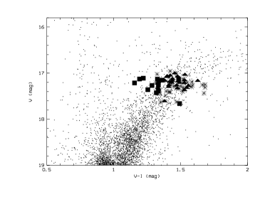
Figure 1: V (V$-$I) color-magnitude diagram of the Disk region (following SMH02), with our sample stars overplotted: asterisks are stars with [Fe/H]${}_{CaT}\geq-0.5$ dex, triangles$-1.0\leq$[Fe/H]${}_{CaT}<-0.5$ dex, squares [Fe/H]${}_{CaT}<-1.0$ dex.

2.2 Observations and reductions

The observations were made at the VLT Kueyen (UT2) telescope at Paranal during the Science Verification of FLAMES/GIRAFFE (Pasquini et al. 2000) in January, February and March, 2003, complemented by one night of the Paris Observatory Guaranteed Time Observations in January, 2004. In its MEDUSA mode, GIRAFFE is a multiobject spectrograph with 131 fibers of which 67 were used for the present project. The remaining fibers were allocated to targets of other Science Verification projects in the LMC. The detector is a 2048 $\times$ 4096 EEV CCD with 15$\mu$m pixels. We used the high resolution grating of GIRAFFE in three different setups: (i) H14 $\lambda$638.3 - $\lambda$662.6 nm with R=28800; (ii) H13 $\lambda$612.0 - $\lambda$640.6 nm with R=22500, and (iii) H11 $\lambda$559.7 - $\lambda$584.0 nm with R=18529. Exposure times are 6 hours for H14 and H13 setups and 7h30 for H11. The setups were chosen in order to cover the maximum number of key elements such as Fe I and Fe II for spectroscopic calculations of stellar parameters, and $\alpha$, iron-peak and $s$-process elements, for the abundance analysis. The average signal to noise ratio of the spectra is S/N$\sim$80 per resolution element.

The data reduction was carried out using the BLDRS (GIRAFFE Base-Line Data Reduction Software http://girbldrs.sourceforge.net/) and consists of bias subtraction, localization and extraction of the spectra, wavelength calibration and rebinning. We have also used the MIDAS packages for sky subtraction and co-addition of individual exposures.

3 Determination of stellar parameters

3.1 Photometric stellar parameters

A first guess of the stellar parameters was made using photometric data of CTIO (V,I from SHM) and 2MASS (J,H,K). Bolometric magnitudes and effective temperatures were derived from calibrations of Bessell, Castelli & Plez (1998, hereafter BCP). The observed CTIO and 2MASS colors were transformed into the corresponding photometric systems using Fernie (1983, V$-$I Cousins to Johnson) and Carpenter (2001, K, V$-$K & J$-$K 2MASS). Photometric data are given in Table Chemical abundances in LMC stellar populations I. The Inner disk sample , while Table Chemical abundances in LMC stellar populations I. The Inner disk sample gives the derived effective temperatures (T_phot) and surface gravities (log g_phot): T_phot is derived using the BCP calibration of the deredenned V$-$I and V$-$K colors, and the surface gravity is computed using the following relation:

$$\log{\rm g_{phot}=4.44+log(M)+4\times log(T_{phot}/5790.)+0.4\times(M_{bol}-4.75)},$$

where $\rm M_{bol}$ is computed from the dereddened K magnitude of the star, the bolometric correction BC_K taken from BCP, and the mass of the stars (M) are assumed to be 2M$\sun$. A distance modulus based on Hipparcos data and the period-luminosity relations from LMC Cepheids of 18.44 $\pm$ 0.05 mag is assumed (Westerlund 1997, Madore & Freedman 1998). Uncertainties of this value stems from the specific subsets of the Cepheids chosen for the comparison (Madore & Freedman 1998). For the reddening, two values were checked: E(B$-$V) = 0.03, which was derived by SMH02 for the sample of the Inner Disk, using Strömgren photometry, and E(B$-$V) = 0.06, a mean value for the whole disk (Bessell 1991). We adopted CaT metallicities from SMH as our initial guesses and reported them in the [Fe/H]_CaT column of Table Chemical abundances in LMC stellar populations I. The Inner disk sample .

We have derived temperatures from V$-$I, V$-$K and J$-$K colors. We have found some trends when comparing temperatures from different colors: T_eff(V$-$I) is 65K hotter than T_eff(V$-$K) in the mean, with $\sigma$=59K; T_eff(J$-$K) is 21K hotter than T_eff(V$-$K) and shows a highly dispersed relation, with $\sigma$=118K (these numbers vary only slightly when choosing a reddening of E(B$-$V)=0.06 or 0.03). As initial values of our stellar temperatures we have chosen to use a weighted mean of the estimates from V$-$I and V$-$K, omitting the less sensitive J$-$K color. We assign higher weight to the more temperature-sensitive (V$-$K), according to the following expression:

$${\rm T_{eff}=(T_{eff}(V-I)+2\times T_{\rm eff}(V-K))/3.}$$

In Table Chemical abundances in LMC stellar populations I. The Inner disk sample the inferred temperatures for the two values of reddening, T_photLow and T_phot for E(B$-$V) = 0.03 and 0.06 respectively, are given.

3.2 Spectroscopic parameters

The final stellar parameters used for the abundance determination of the sample stars were derived spectroscopically using abundances derived from the equivalent widths (EW) of iron lines. Although 67 stars were observed, 8 of them have one or two setups with low S/N, compromising the determination of stellar parameters. These stars have not been included in the abundance analysis. Due to low S/N ratios, the H13 setup has not been used for the following stars: RGB_601, RGB_646, RGB_672, RGB_699, RGB_705, RGB_710, RGB_720, RGB_731, RGB_748, RGB_756, RGB_773 and RGB_775; and for RGB_666 the H11 setup has been discarded. We have estimated the stellar parameters as follows: effective temperatures are calculated by requiring no slope in the A(Fe I) vs. $\chi_{exc}$ (excitation potential) plot ($\chi_{exc}$ is the excitation potention of the line); microturbulent velocities, $\rm V_{\rm t}$, are derived demanding that lines of different EW give the same iron abundance, also checking for no slope in the [Fe/H] vs. log(W/$\lambda$) plot (iron abundance vs. the reduced equivalent width); and surface gravities are determined by forcing the agreement between Fe I and Fe II iron abundances (within the accuracy of the abundance determination of Fe II). For the temperature and surface gravity ranges covered by our current sample of stars, T_eff and log g determinations are well correlated and the calculation of stellar parameters is made iteratively. In Fig. 2 we show an example of the excitation equilibrium calculation for RGB_625, and in Fig. 3, the [Fe/H] vs. $\lambda$ with the log(W/$\lambda$) check, and the [Fe/H] vs. EW are given for RGB_710. The spectroscopic and photometric parameters of all our stars are reported in Table Chemical abundances in LMC stellar populations I. The Inner disk sample , together with the barycentric radial velocities calculated from the spectra.

Figure 2: Example of the temperature calculation for RGB_625: [Fe I/H] vs. $\chi_{exc}$.

Figure 3: Examples of microturbulence velocity calculation for RGB_710: [Fe I/H] vs. $\lambda$ (left); and [Fe I/H] vs. EW (right). The different values for the reduced EW in the left panel are given with different symbols: 1) squares: -5.6 $\leq$ log W/$\lambda$ $\leq$ -5.0 and 12$<$W$<$50; 2) crosses: - -4.8 $\leq$ log W/$\lambda$ $\leq$ -4.0 and 80$<$W$<$300; and 3) times: -5.0 $\leq$ log W/$\lambda$ $\leq$ -4.8 50$<$W$<$80.

3.2.1 Equivalent widths, line list and model atmospheres

The EW of the lines and the radial velocities (RV, in km/s, reported in Table Chemical abundances in LMC stellar populations I. The Inner disk sample ) of the stars are computed using the program DAOSPEC written by Stetson (Stetson and Pancino, in preparation). The line list and the atomic data were assembled from the literature and the oscillator strengths references are given in Table Chemical abundances in LMC stellar populations I. The Inner disk sample . DAOSPEC has already been used to measure the EW of spectra for different types of stars yielding reliable results (e.g. Pasquini et al. 2004, Barbuy et al. 2006, Sousa et al. 2006). We have made a study of the DAOSPEC EW estimations using GIRAFFE spectra. In the Appendix A we show a comparison of DAOSPEC EW with those made by hand using the Splot - Iraf task for six of our sample stars. We have found a very good agreement between the two methods for the analysis of the GIRAFFE spectra within the expected uncertainties.

MARCS 1D plane-parallel atmospheres models Gustafsson et al. 1975, Plez et al. 1992, Gustafsson et al. 2003) were kindly provided by B. Plez (private communication).

3.2.2 Comparison with UVES analysis

In a previous observing run (066.B-0331), we obtained UVES spectra (in slit mode) for one of our sample stars, RGB_666. UVES is an echelle spectrograph also mounted on the VLT Kueyen telescope with a higher resolving power: R = 45000 (with a slit of 1$\arcsec$) and a much wider wavelength coverage (in the case of our chosen set-up, 4800-6800Å), and therefore with a better performance to derive equivalent widths. We have used this spectrum to evaluate DAOSPEC performance to derive EW from low resolution spectra. In Fig. 4, equivalent widths derived with DAOSPEC from UVES spectra from 5800 to 6800Å are compared to those measured also by this program on the GIRAFFE spectra of the same star using the same line list. In the top of the plot, the mean differences between analyses are given together with the dispersion and the number of lines used (lines of all elements are plotted in this comparison). We can see from this plot that GIRAFFE EW are only slightly higher than UVES EW. Such a difference is probably due to a better definition of the continuum for the UVES spectra, as well as the increased blending at the lower resolution of GIRAFFE. Using the EW of this figure, we have inferred the stellar parameters for UVES to compare the analysis from both spectrographs. We have found that the stellar parameters are almost identical to those given for RGB_666 in Table Chemical abundances in LMC stellar populations I. The Inner disk sample , except for V_t for which we have found V_t = 1.8 kms^-1 (a difference of $\Delta$ V_t = +0.1 kms^-1) . Comparing the results from the two spectrographs, we have: [FeI/H]_UVES-[FeI/H]_GIRAFFE = -0.11 dex and [FeII/H]_UVES-[FeII/H]_GIRAFFE = 0.00 dex. Therefore it is possible that a systematic uncertainty of [Fe/H] $\sim$ 0.1 dex may be present in the following abundance analysis, although robust statements on this uncertainty would require better statistics. Let us further note that this 0.1 dex difference is within the errorbar that we quote for our GIRAFFE metallicities.

Figure 4: Comparison between UVES and GIRAFFE spectra analyses for RGB_666.

3.3 Behavior of stellar parameters

We found good agreement between spectroscopic and photometric temperatures. Our spectroscopic temperatures are hotter than photometric temperatures derived using the low reddening value, T_photLow, by 113 K, with $\sigma$=91K, and by 54K than T_phot (higher reddening value) with $\sigma$=64K. An interesting result is depicted in Fig. 5 where we compare the spectroscopic temperatures T_eff(spec) with those derived from colors, T_eff(V$-$I) and T_eff(V$-$K), and from the equation given in Sect. 3.1.1, T_eff(phot), for both values of reddening (E(B-V)=0.06 in the upper panels, and E(B-V)=0.03 in the lower panels). This figure shows that photometric temperatures inferred using E(B$-$V) = 0.06 are in much better agreement with spectroscopic temperatures than those derived with the lower E(B$-$V). Provided that the photometric temperatures and the excitation temperature scale show a good agreement, this could indicate that E(B$-$V)=0.06 is a better reddening value for this region.

Figure 5: Comparison between photometric and spectroscopic temperatures (see text). On the bottom plots, photometric temperatures are derived with E(B$-$V)=0.03 (SMH02), while on the upper plots, photometric temperatures are derived with a higher reddening value, E(B$-$V)=0.06 (Bessel 1991). Solid lines represent T_eff(spec) = T_eff(phot) and T_eff(spec) = T_eff(phot) $\pm$ 100K.

On average, spectroscopic surface gravities are lower than the photometric estimates by $\rm\Delta(\log g_{spec}-\log g_{phot})=-0.38$ dex, as might be expected if NLTE overionization effects are at work (Korn et al. 2003). This systematic effect in log g corresponds to a 0.2 dex difference between FeI and FeII.

The metallicities that we derive differ on average from those derived from the CaT by $\rm\Delta([Fe/H]_{CaT}-[Fe/H]_{spec})=+0.13$ dex with $\sigma$= 0.27 dex. In fact, most of this effect comes from the high-metallicity end of the sample: for [Fe/H]${}_{\rm CaT}>-0.6$ dex, CaT seems to overestimate the metallicity systematically by 0.27 dex ($\sigma$= 0.19 dex), whereas for the metal-poor end of the sample, there is almost no systematic effect ($\rm\Delta[Fe/H]_{CaT}-[Fe/H]_{spec})=-0.04$ dex with $\sigma$= 0.24 dex.

Finally, in Fig. 6, abundance ratios of different species, [Cr/Fe], [Ni/Fe] and [V/Fe], against temperatures are plotted in order to check the quality of the spectroscopic temperatures. As can be seen from this picture, there is no trend of the abundances of the elements with temperature, which means that our temperatures are well defined. Our final sample comprises 59 red giant stars within $-1.7<{\rm[Fe/H]}<-0.30$ dex and temperatures ranging from 3900 K to 4500 K.

Figure 6: Abundance ratios against temperatures. From top to bottom: [Cr/Fe] vs. T_eff, [Ni/Fe] vs. T_eff and [V/Fe] vs. T_eff.

4 Abundance determination

We have selected a list of lines covering the chosen setups in order to sample as much as possible the most important elements: iron-peak, neutron-capture and $\alpha$ elements. Abundances are derived from EW mesurements for eight elements (in parenthesis the average number of lines used in the analysis): Fe (45), Ni (7), Cr (4), V (11), Si (3), Ca (10), Ti (7) and Na (3). We have also derived abundances by using line synthesis for nine elements (in parenthesis the lines used in the synthesis): O ([O I] 6300$\rm\AA$); Mg I (5711 $\rm\AA$), Co I (5647 $\rm\AA$), Cu I (5782 $\rm\AA$), Sc II (5657 $\rm\AA$), La II (6320 $\rm\AA$), Y II (6435 $\rm\AA$), Ba II (6496 $\rm\AA$), and Zr I (6134 $\rm\AA$). The code used for the abundance analysis was developed by Monique Spite (1967) and has been improved over the years. We note that both model atmospheres and the line synthesis program are in spherical geometry, so errors due to geometry inconsistencies are minimized (Heiter & Eriksson 2006). For the synthesis of the [O I] line in 6300.311 $\rm\AA$, we have taken into account the blend with Ni I 6300.336 $\rm\AA$ (line data from Allende Prieto 2001), but no difference have been detected between results with or without such blend. Hyperfine structures (HFS) are taken into account for the following elements (the line sources are given in parenthesis): Ba II (Rutten 1978, and the isotopic solar mix following McWilliam 1998); La II (Lawler et al. 2001 with log gf from Bord et al. 1996); Cu (Biehl 1976), and Co I and Sc II (Prochaska et al. 2000). In Fig. 7 the fitting procedure is shown for the Y I 6435$\rm\AA$ line in RGB_752 and the La II line 6320$\rm\AA$ in RGB_690. Abundances are given relative to solar abundances of Grevesse & Sauval (2000). Atomic lines for the synthesis have been chosen according to the quality of the synthetic fit in the Solar Flux Atlas of Kurucz et al. (1984). In Tables 4 to 7 the derived abundances are given.

Figure 7: Example of the line synthesis procedure for the Y I and La II lines: left panel: Y I $\lambda$6435$\rm\AA$ line fitting for RGB_752; right panel: La II$\rm\AA$6320 line fitting for RGB_690. The black circles depict the observed spectra and the lines are the synthetic spectra. Abundances of the synthetic spectra are: [Y/Fe] = $-$0.55 (dashed line), $-$0.45 (continuous line - best fit), $-$0.25 (dotted line); and [La/Fe] = 0.56 (dashed line), 0.66 (continuous line - best fit), and 0.76 (dotted line).

Errors in the derived abundances have three main sources: the uncertainties in the stellar parameters, the uncertainties in the measurements of the EW (or spectrum synthesis fitting) and the uncertainties on the physical data of the lines (mainly $\log$ gf). The errors due to stellar parameters uncertainties have been chosen as the maximum range each parameter could change not to give unrealistic models atmospheres. The errors $\rm\delta([X/Fe])_{model}$, are given in Table 8, assuming the following uncertainties in each of the stellar parameters: $\Delta$(T_eff) = $\pm$100K, $\Delta$(log g) = $\pm$0.4 dex, $\Delta$(V_t) = $\pm$0.2 km/s and $\Delta$([Fe/H]) = $\pm$0.15 dex.

Errors in the EW measurement are computed by DAOSPEC during the fitting procedure, then propagated into an abundance uncertainty for each line, and then combined into an abundance error on the mean abundance for each element ($\delta_{\rm DAOSPEC}$). Errors due to the combined uncertainties on the line data and line measurement are reflected in the abundance dispersion observed for each element, provided that the number of lines is large enough to measure this dispersion in a robust way (N$\geq$3). We therefore combined these error estimates in a conservative way as given bellow:

$${\begin{array}[]{ll}\rm N_{X}<3:&\delta([X/H])=\delta_{DAOSPEC},\\ \rm N_{X}\geq 3:&\delta([X/H])=Max(\delta_{DAOSPEC},\frac{\sigma(X)}{\sqrt{N_{X}}})\\ \end{array}}$$ (1)

where $\rm N_{X}$ is the number of lines of the element X and $\sigma(X)$ the dispersion among lines.

These errors are calculated for each element and given in Tables 4 to 6 together with the abundances derived from the EW. For elements measured by synthesis spectrum fitting, an error estimate has been carried out of the typical abundance change for which two different synthetic spectra (i.e. computed with two slightly different abundances) still fit satisfactorily the same line. On average, these values are the following for each element: ${\delta}$[Zr/H] = 0.15 dex; ${\delta}$[Y/H] = 0.15 dex; ${\delta}$[La/H] = 0.20 dex; ${\delta}$[Ba/H] = 0.25 dex; ${\delta}$[Co/H] = 0.10 dex; ${\delta}$[Cu/H] = 0.20 dex; ${\delta}$[Sc/H] = 0.10 dex; ${\delta}$[Mg/H] = 0.15 dex and ${\delta}$[O/H] = 0.20 dex. For the error bars reported in our abundance plots (always shown in the lower left corner of Figs. 8-12) we have adopted two error sources. The first, due to stellar parameter uncertainties (leftmost side of the plots), comes directly from Table 8, whereas the second (more to the right side) represents the error associated with the abundance analysis. For those abundances derived from the EW, this is the mean error of Tables 4,5, and 6, and for those elements with abundances derived from spectrum synthesis, it is the value described earlier on in this Section.

5 Abundance Distributions and comparison to Galactic samples

In Figs. 8 to 12 we depict the elemental distributions for the $\alpha$-elements, the iron-peak group, Na, Sc, Cu and $s$-elements for our stars compared to different samples of the Galaxy and the LMC. Our data are represented as dots. The references of the disk are: Fulbright 2000 (crosses); Reddy et al. 2003 (open squares); Allende Prieto et al. 2004 (open stars); Prochaska et al. 2000 (open triangles); Burris et al. 2000 (stars - only for the heavy-elements plots); Johnson & Bolte 2002 (open trianlges - only for the heavy-elements plots); Simmerer et al. 2004 (open hexagons); Nissen & Shuster 1997 (asterisks, only stars with low [$\alpha$/Fe] ratios); Nissen et al. 2000 (asterisks - Sc abundances for the low-$\alpha$ stars ); and Bensby et al. 2004 (open squares - only for the oxygen plot). LMC globular clusters (GC) stars from Hill et al. (2000, hereafter HI00) for O, and Hill (2004 hereafter HI04) for Na, Mg, Ca and Si are plotted as downward-pointing, open triangles; LMC GC stars from JIS06 are represented as open diamonds; field LMC red giants of SM02 are depicted as open pentagons. Error bars as described in Sect.4.0.1 are shown in the lower left side of the plots.

5.1 Ca, Si and Ti

In Fig. 8, the elemental distributions for Ca I, Si I, and Ti I are depicted. We have found that [Si/Fe] follows roughly the solar ratio with some scatter. [Ca/Fe] shows a slight decrease with metallicity. Compared to the distribution of the galactic halo, both silicon and calcium mean abundances are deficient by a factor of 3. Ti I ratios are also underabundant relative to galactic disk and galactic halo samples, and agree very well with the results of SM02, who derived titanium abundances from neutral lines for a sample of red giants from LMC disk. There is a hint of a decreasing trend of Ti abundances for higher metallicity stars, especially when SM02 datapoints are taken into account together with our sample. Compared to the LMC GC of H04, we have found that the star of our sample with metallicity similar to those of those of Hill et al. (2004) also has similar [Ca/Fe] ratio. The JIS06 sample of LMC GC stars seems to overlap our [Ca/Fe] and [Ti/Fe] distributions, while their [Si/Fe] ratios are enhanced.

A very interesting result emerges when comparing our data with those of Nissen & Shuster 1997 (hereafter NS97, asterisks). NS97 discovered a sample of stars from the galactic halo with abnormal abundances: low [$\alpha$/Fe], [Na/Fe] and [Ni/Fe] ratios compared to “standard” halo stars. Such chemically peculiar or “low-$\alpha$” halo stars have an important role in elucidating the possible merging history of the galactic halo. Because of their chemical properties, they indicate that this group have formed in another stellar system that evoveld separately, and which has been captured or ejected to the halo. Comparing our LMC distribution to the low-$\alpha$ stars, we have found that NS97 stars show a slightly enhanced mean $\alpha$ abundance relative to our LMC stars.

Si, Ca and Ti are predicted to be produced in intermediate mass Type II SNe (SNe II) with a smaller contribution from Type Ia SNe (SNe Ia) (e.g. Tsujiomoto et al. 1995, Thielemann et al. 2002), while Fe is mostly produced by SNe Ia (e.g. Thielemann et al. 2001, Iwamoto et al. 1999). The low [$\alpha$/Fe] ratios observed indicate that SNe Ia have contributed more to the ISM content in the past than the SNe II.

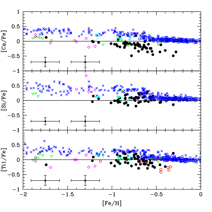
Figure 8: Abundance distributions for the Inner Disk LMC stars: [$\alpha$/Fe] vs. [Fe/H] (blue dots). LMC samples are depicted with polygons (downward-pointing green triangles - Hill et al. 2000; red pentagons - Smith et al. 2002; magenta diamonds - Johnson et al. 2006); and the remaining symbols (all in blue) are data for the galactic stars (crosses - Fulbright 2000; open squares - Reddy et al. 2003; cyan asterisks - Nissen & Schuster 1997). Error bars depict: a. leftmost side of the plots - errors due to stellar parameter uncertainties (Table 8); and b. more to the right side - errors associated with the abundance analysis - for those derived from the EW, is the mean error of Tables 4,5, and 6; for those elements with abundances derived from spectrum synthesis, is the value described in Sect. 4.

5.2 Mg, O, Na and Sc

In Fig. 9, abundance ratios are given for O, Mg, Sc and Na. Nucleosynthetic predictions attribute the main source of O, Mg and Na to high-mass stars, with M $>$ 25 M_⊙, which explode as SNe II (Woosley & Weaver 1995, hereafter WW95), with Na production controlled by the neutron excess. Although WW95 have attributed the origin of Sc to SNe II, the main source of Sc production is still unclear (e.g. McWilliam 1997, Nissen et al. 2000).

As can be seen in the upper panel of Fig. 9, oxygen ratios fall in the lower envelope of the galactic halo and disk distributions. For higher metallicities, it shows a faster decline with metallicity compared to stars from the galactic disk. In the second plot we see that the [Mg/Fe] ratios for the LMC Inner Disk overlap those of the Galaxy, but with smaller mean values. In contrast, Na and Sc behaviors are similar to those of the $\alpha$-elements Ti, and Si. Both elements are deficient and show smaller values for higher metallicities, while for the metal-poor tail, a match to the Galactic samples is observed. From this figure we see that the different LMC samples agree very well for all elements, Mg, O, Na and Sc, even the LMC globular clusters of H00, H04 and JIS06. A few stars in the NS00 sample of low-$\alpha$ stars show small [Sc/Fe] ratios and overlap our sample, but most of them show solar [Sc/Fe] values, higher than in our LMC sample. Sodium abundances in NS97 sample are similar to our values, although with a higher mean abundance. It is important to notice that sodium abundances in giants are still uncertain. Pasquini et al. (2004) found that [Na/Fe] ratios in giant stars are slightly higher than those from dwarf stars in the same cluster. High [Na/Fe] ratios were also inferred from giants in M67 (Tautvaišiene et al. 2000). But such results have not been confirmed in the reanalysis of [Na/Fe] in giants and dwarfs of M67 (Randich et al. 2006).

Nissen et al. (2000) also found that Sc behaves similarly to Na, showing lower [Sc/Fe] ratios in their low-$\alpha$ stars, suggesting a correlation among those elements. In order to test the hypothesis of a correlation among Na and $\alpha$-elements, and Sc and $\alpha$-elements we have applied a statistical test to check for the existance and significance of such correlation, calculating the linear correlation coeficient, which varies from 1 or -1 (maximum correlation or anti-correlation) to 0 (no correlation). We have found that the correlations are weak: for Na-Ca, a correlation coefficient $\phi$ = -0.06 is found, and for Sc-Ca, $\phi$ = 0.39.

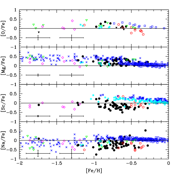
Figure 9: Abundance distributions for the Inner Disk LMC stars: [ O, Mg, Na, Sc/Fe] vs. [Fe/H] (symbols are the same as in Fig. 8, and we added: blue open stars - Allende Prieto et al. 2004, blue crosses - Bensby et al. 2004 only for oxygen; cyan asterisks - Nissen et al. 2000 for Sc and Nissen & Schuster 1997 for the other elements).

5.3 Iron-peak elements

Abundance distributions for the iron-peak elements are shown in Fig. 10. The iron-peak elements Co, Ni and Cr display a very distinct pattern in the LMC Inner Disk stars, with underabundant values compared to the Galactic distributions and many subsolar ratios. [Co/Fe], [Cr/Fe] and [Ni/Fe] show a flat trend for most of the metallicity range, with mean abundances of $\sim$ -0.18 dex for Cr, $\sim$ -0.24 for Ni, and $\sim$ -0.14 dex for Co. The [V/Fe] ratios are similar to the galactic halo and disk patterns and track the solar value, with a group of stars showing smaller values. Results from the LMC GC of JIS06 seem to agree with our samples for Co, Ni and Cr. Vanadium in their sample shows an offset, with abundance ratios corresponding to the stars with smaller values in our sample. NS97 low-$\alpha$ stars overlap our sample for Ni and Cr, but lie in the high abundance envelope of the distributions.

According to nucleosynthetic predictions, iron-peak elements are mainly produced in SNe Ia (Iwamoto 1999, Travaglio et al. 2005): while each SN Ia produces $\approx$ 0.8 M_⊙ of the solar iron-peak elements, SN II produce $\approx$ 0.1 M_⊙ each (Timmes et al. 2003). The difference in the distributions from one environment to the other are an evidence that the production factors for each iron-peak element are not the same in the different types of SNe and depend on the SFH of the parent population. This will be further discussed in Sect. 7.

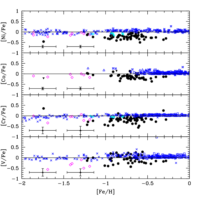
Figure 10: Abundance distributions for the Inner Disk LMC stars: [Iron-peak/Fe] vs. [Fe/H] (symbols are the same as in Figs. 8 and 9, and the solid downtriangles depict upper limits for our sample stars).

5.4 Copper

In Fig. 11 we show the plot for Cu. We have found that in the Inner Disk LMC stars, the copper distribution is flat, with a mean value of [Cu/Fe] = $-$0.68 dex. Comparing to the Galaxy, there is an overlap between the LMC and Halo stars at the metal-poor end ([Fe/H] $<-1.3$ dex); for the higher metallicity range, the distributions diverge, with LMC stars showing a clear underabundance with respect to the Galactic Disk. JIS06 also found an offset in their [Cu/Fe], compatible to our abundance ratios.

Although originally associated with the iron-peak elements, the origin of copper is still much-debated (e.g. Bisterzo et al. 2004, Cunha et al. 2004, Mishenina et al. 2002). Sometimes its main source is attributed to SNe Ia (Matteucci et al. 1993, Cunha et al. 2002, Mishenina et al. 2002) and sometimes to SNe II, particularly to a metallicity dependent mechanism (Bisterzo et al. 2004; McWilliam & Smecker-Hane 2005). If the elemental behavior of the present sample, with low [$\alpha$/Fe], low [iron-peak/Fe] ratios, is due to a higher contribution from SNe Ia, the overall low [Cu/Fe] pattern indicates that thermonuclear supernovae cannot be the main source of Cu production.

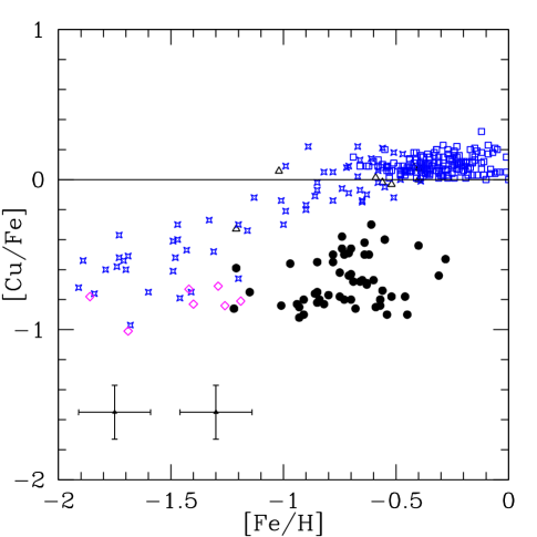
Figure 11: Abundance distributions for Inner Disk LMC stars: Copper. The symbols are the data from: our sample stars (dots); Mishenina et al. 2002 (blue stars); Prochaska et al. 2002 (open blue triangles); Reddy et al. 2003 (open blue squares); Johnson et al. 2006 (magenta diamonds).

5.5 $s$-process elements

We have found interesting elemental distributions for the $s$-process elements for our sample stars (Fig. 12). While the light $s$-process elements (hereafter $ls$: elements made by the $s$-process with atomic number lower than $\sim$45) Zr and Y, show subsolar ratios with mean abundances the heavy $s$-process elements (hereafter $hs$: elements made by the $s$-process with atomic number higher than $\sim$50) La and Ba show supersolar values with enhanced pattern compared to those of the Galaxy. The underabundance of $ls$ elements is quite strong, [Y/Fe] = $-$0.33 dex and [Zr/Fe] = $-$0.48 dex, and Zr shows a hint of decreasing with increasing metallicities. Of the $hs$ elements, Ba has a peculiar behavior with a high value for one metal-poor star ([Fe/H] $<-1.4$ dex), mild enhancements until [Fe/H] $\sim-$1.15 dex, increasing again towards higher metallicities. La shows no trend with metalicity, with mild enhancements everywhere. One star, RGB_1118, has particularly high La and Ba abundances ([Ba/Fe] and [La/Fe]$\geq$+1.0 dex) and could be a star enriched in $s$-process elements (via mass-transfer from a former AGB companion), although it is not possible from our present data to discriminate between enhancements of $s$-process or $r$-process elements. The $s$-process elements in JIS06 sample are different when compared to our results. While they have found no offset for the $ls$ elements compared to the galactic distribution, showing therefore a higher abundance compared to our stars, their $hs$ elements (Ba and La) are less enhanced than ours. Comparing NS97 low-$\alpha$ stars with our sample, we find that these stars show abundances nearer those of normal disk stars for Ba and Y than the LMC stars.

The $hs/ls$ ratios are high, showing large scatter, with a mean value of [$hs/ls$] = +0.77 dex, as can be seen in Fig. 13. This is very different from what is observed for the galactic halo and disk stars, which fall around -0.2 to +0.2 dex (e.g. Pagel & Tautvaišiene 1997; Travaglio et al. 2004). A slow increasing trend with metallicity is observed.

High abundances of elements heavier than Zr were also derived for LMC and SMC supergiants (Russell & Bessell 1989; Spite et al. 1993; Hill et al. 1995). Hill et al. (1995) for example, found that the light $s$-elements Zr and Y show solar composition in LMC supergiants while heavier $s$-elements (Ba, La, Nd) as well as the $r$-process element Eu are enhanced by +0.30 dex. As discussed by these authors, the overabundance of the heavier $s$-process and $r$-process elements seems to be a characteristic of the Magellanic Clouds, and indicate a particular evolution of that galactic system, although no satisfactory explanation was proposed for it.

In order to evaluate the $r$-process and $s$-process contributions within our sample we analysed the $r$-process content of one of our sample stars for which we have UVES spectra that cover the Eu $\lambda$ 6645 $\rm\AA$ line. Eu and Ba abundances were derived from these spectra in the same way as was done for GIRAFFE spectra. For RGB_666 we find respectively [Ba/Fe] = $+$0.52, and [Eu/Fe] = $+$0.40 dex. The corresponding [Ba/Eu] ratio of 0.12 (to be compared with the solar $r$-process [Ba/Eu]=$-$0.55 and the solar $s-$process [Ba/Fe]=+1.55, following Arlandini et al. 1999), indicate that this star contains a significant $r$-process contribution at a value close to the solar $s$/$r$ mix at intermediate metallicities (RGB_666: [Fe/H]=-1.10).

A high content of $r$-process elements seems to be in contradiction with the observed low [$\alpha$/Fe] ratios (both being produced in massive stars). More data on Eu abundances are needed to confirm this high content of $r$-process elements, and in particular, the trend of the $s$/$r$ fraction (traced by [Ba/Eu]) as a function of metallicity will help to constrain the source of the high content of heavy $s$-process elements in the LMC disk. We intend to tackle this issue in the two other fields (Bar and Outer Disk) of our LMC program, since one of the MEDUSA wavelength ranges covers the Eu line for these fields.

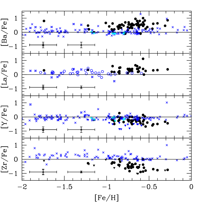
Figure 12: Abundance distributions for Inner Disk LMC stars: [$s$-elements/Fe] vs. [Fe/H]. The large dots (or downtriangles for upper limits) depict our sample stars, while open blue symbols represent galactic samples: symbols as in Figure 8, plus Burris et al. 2000 (blue stars); Johnson & Bolte 2002 (blue trianlges); Simmerer et al. 2004 (blue hexagons); Nissen & Schuster 1997 (cyan asterisks).

Figure 13: Observed abundance ratios [$hs$/$ls$] = [Ba+La/Y+Zr].

5.5.1 The NaMg, NaNi relations

In the paper by NS97 the authors found a correlation between Na and Ni for their halo stars (both “normal” and “low-$\alpha$” stars). Such correlation has been confirmed for a group of stars in the Dwarf Spheroidal Galaxies (Shetrone et al. 2003, SH03, Tolstoy et al. 2003, TO03, Venn et al. 2004). To evaluate this trend, we plot in Fig. 14 the [Ni/Fe] vs. [Na/Fe] relation for our sample stars (dots) together with NS97 low-$\alpha$ stars. We see that the LMC stars also show a correlation between Na and Ni, although with a flatter pattern than the increasing trend observed for the NS97 sample. According to Tsujimoto et al. (1995), Ni can be produced in SNe Ia without Na production; therefore, a higher contribution from SNe Ia would flatten the NaNi relation (Venn et al. 2004) and could explain the behavior of the LMC stars. In Fig. 14 we also analyze the correlation between Na and Mg and we find decreasing [Na/Mg] ratios for increasing [Mg/H] ratios. The NS97 low-$\alpha$ stars seem a continuation of the observed trend.

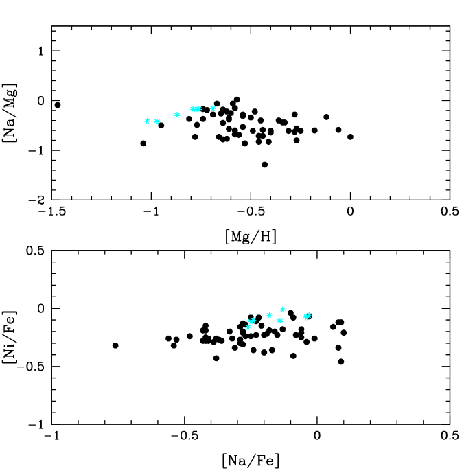
Figure 14: The NaNi and NaMg abundance relations. Our sample stars are depicted as dots and NS97 low-$\alpha$ stars as starred symbols.

6 Comparison to the Dwarf Spheroidal Galaxies

In Figs. 15 and 16 we show a comparison of the chemical distributions of our LMC sample to those of the dSph galaxies of Shetrone et al. (2003) and Tolstoy et al. (2003), and the Sagittarius dwarf galaxy (Sgr) of Bonifacio et al. (2004) and Sbordone et al. (2007). The elemental distributions of most dSph galaxies are more concentrated in the metallicity range for which we have the lowest number of stars, [Fe/H] $<-1.2$, so the present analysis is not ideal. In Fig. 15 the distributions for the $\alpha$-elements Ca, Ti and Si and for Cu are depicted (the description of the different symbols are given in the figure captions). As can be seen from these figures, and observed for also for O, Mg, Na and Sc, there is an overlap among the LMC abundance ratios and those of the dSph galaxies. The same occurs for the iron-peak elements Cr, V and Ni and for Cu (with the exception of Fornax, which shows higher values for Cu). Particularlly, the agreement among our data and those of the Sagittarius dwarf galaxy is very good, except that this galaxy shows [Ti/Fe] and [Mg/Fe] ratios slightly underabundant relative to our values.

For the $s$-process elements, depicted in Fig. 16, the dSph galaxies show enhanced $hs$ and deficient $ls$ compared to the Galactic behavior, although the general pattern is less discrepant than that showed by the LMC inner disk stars, except for Sgr, which shows striking similar ratios when compared to our data. Fornax has a more metal-rich star (Fnx21) with high $s$ content, which may be an $s$-enriched star. The [Ba/Y] ratios show a large offset relative to galactic samples, of the same order magnitude we have found. Venn et al. (2004) attribute such offset to primary $s$-process production by low-metallicity AGB stars.

The very similar elemental distributions of the Sgr galaxy indicate that this galaxy must have been very similar to LMC, i.e., with a higher mass content, which may be nowadays hidden in streams and/or dynamically mixed to the Galaxy.

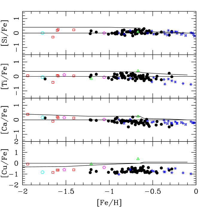
Figure 15: Comparison of the Inner Disk LMC stars with stars from the dwarf spheroidal galaxies and the Sgr galaxy. 1. Alpha elements. The symbols are: our sample (dots), Leo I (magenta pentagons), Sculptor (open cyan dots), Fornax (green triangles), Carina (red squares), and Sgr (Bonifacio et al. 2005 - blue stars; Sbordone et al. 2007 - blue asteriks). Solid lines depict mean values of the Galactic distributions for each element.

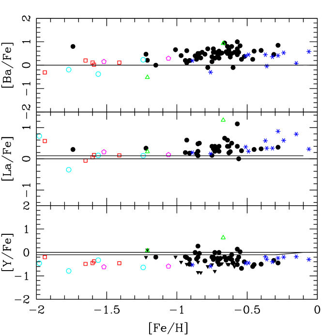
Figure 16: Comparison of the Inner Disk LMC stars with stars from the dwarf spheroidal galaxies. 2. $s$-process elements (symbols are the same as in Fig. 15).

7 Discussion

It is an amazing opportunity to have so much data on the amount of various elements of stars in an external galaxy. With this unique dataset, we can now explore in more detail the SFH and better understand the evolution of the LMC disk. The overall low [X/Fe] ratios indicate that such stars have undergone a global process which is different from that experienced by the average halo and disk stars in the Galaxy. In this section we discuss the possible explanations for such behavior.

We have found an overall low abundance pattern for the $\alpha$-elements, in agreement with many previous works with stars in this galaxy (Sect. 1). The heavy $s$-elements show an enhancement relative to the Galactic disk distributions, as inferred before for supergiants and red giants in the LMC. New results from the present work include low light-$s$ abundance ratios ([Y/Fe] and [Zr/Fe]), with most of the stars showing subsolar values, and an unexpected offset for the iron-peak elements Ni, Cr and Co, and in some stars, also for V. Na and Sc are deficient with many subsolar ratios relative to iron, and copper shows a very low abundance in all stars from the present sample, with mean [Cu/Fe] $\sim$ -0.7 dex, and no trend with metallicity.

As seen in previous sections, small [$\alpha$/Fe] ratios have already been observed in other stellar systems such as the chemically peculiar halo stars (NS97, NS00), the dSph galaxies of the Local Group (Shetrone 2003, Tolstoy 2003), the Sagittarius galaxy (Smecker-Hane & McWilliam 2002, Bonifacio et al. 2004, Monaco et al. 2005, Sobordone et al. 2007), as in samples in the LMC (e.g. Hill et al. 2000, 2003; SM02, Garnett 2000, Korn et al. 2002). It is interesting to notice that the $s$-process trends in the dSph galaxies (enhanced $hs$ and deficient $ls$ ratios) are the same as for our stars. Correlations between abundances of iron-peak elements and $\alpha$-elements were observed also in other stellar systems. A pattern of slightly deficient Ni and Cr has been observed for the low-$\alpha$ stars of NS97. Bensby et al. (2003) found a correlation among the [iron-peak/Fe] and [Na/Fe] vs. [$\alpha$-elements/Fe] abundance ratios, i.e., sligtly higher [Cr/Fe], [Ni/Fe] and [Na/Fe] ratios in thick disk stars with enhanced [$\alpha$-element/Fe] ratios (see their Fig. 13). Sbodorne et al. (2007) found subsolar ratios for Na, Sc, Co, Ni and V in their analysis of the Sagittarius dwarf galaxy stars, which has also low [$\alpha$/Fe] ratios. Such behavior may tell us interesting details about the formation of these elements and give clues about low-mass galaxy formation.

Many interpretations have been given for the small [$\alpha$/Fe] ratios observed. One hypothesis is that the star formation (SF) developed slowly, in short bursts, followed by long quiescent periods without SF, during which the SNe Ia contaminated the ISM and increased the Fe content (e.g. Gilmore & Wyse 1991). Smaller SNe II/SNe Ia ratios, therefore a higher frequency of SNe Ia relative to SNe II, have also been invoked, within a bursty or continuous regime, and with or without galactic winds (e.g. Pagel & Tautvaišiene 1997, Smith et al. 2002); a steepened IMF relative to that of the solar neighborhood has been proposed by Tsujimoto et al. (1995) and de Freitas Pacheco (1998), whereas alpha-enriched galactic winds, which would lower the [alpha/Fe] content, have been suggested by Pilyugin (1996); and finally, a small (low-mass) star-formation event that would effectively truncate the IMF, yieding fewer high-mass SNe II than produced by normal SF events has been suggested (Tolstoy et al. 2003). To find explanations for the behavior of the iron-peak elements is more puzzling, since they are predicted to be basically produced in SNe Ia (e.g. Travaglio et al. 2005). A possible explanation is that the yields of the SNe Ia are metallicity dependent (Timmes et al. 2003).

The abundance distributions observed for the $hs$ and the $ls$ elements, with $hs/ls$=[Ba+La/Y+Zr], are in agreement with the hypothesis that the $s$-process in AGB stars is metallicity dependent (Busso et al. 1999 and references therein; Busso et al. 2001; Abia et al. 2003, Travaglio et al. 2004). It has been noticed that, due to details of the nucleosynthesis of the $s$-process, $hs$-elements (e.g. Ba, La and Nd) are preferentially produced by metal-poor AGB stars compared to $ls$ elements (e.g. Y, Zr and Sr), which are most efficiently produced at [Fe/H] $\approx$ -0.1 (e.g. Fig. 1 of Travaglio et al. 2004). If the SF is slow, low-metallicity AGB stars have enough time to contaminate the ISM, leaving noticeable chemical signatures for the next generations.

Nevertheless, Venn et al. (2004) discuss the possibility that the abundances of these elements (including Y) in dSph cannot be accounted for solely by the $s$-process, requiring a strong contribution from the $r$-process. Also, according to Richtler et al. (1989) and Russell & Dopita (1992), the most probable explanation for the high Ba and La abundances observed in the Magellanic Clouds is an additional $r$-process component. This would mean that $hs$ and $ls$ elements are produced in different rates by the $r$-process nucleosynthesis, probably in different sites. Therefore, the analysis of the behavior of the $s$-elements in the given metallicity range is complex and must take into account both the $r$ and the $s$ contributions.

7.1 Galaxy Formation and Evolution

One of the most debated themes about galaxy formation in the Universe under a $\Lambda$CDM hierarchical scenario concerns the problem of overprediction of galaxy counts at low-$z$ and underprediction at high-$z$ (Cimatti et al. 2002). One of the consequences for the Local Group is a larger number of small galaxies than is actually observed although the number of dwarf galaxies observed around the Milky Way and M31 has lately grown significantly (eg. Belokurov et al. 2007). According to these models, numerous merging and accretion events play an important role in the formation process of massive galaxies (e.g. Moore et al. 1999), although not all dark matter clumps are predicted to host star formation and thereby become visible galaxies (e.g. Bullock & Johnston 2005). The quest for signatures of possible accreted stars from nearby galaxies in the Galactic halo and disk have been carried out, without definite conclusions (NS97, NS00, Ivans et al. 2003, Venn et al. 2004). A careful inspection of the elemental distributions of the different Galactic components reveals a low dispersion in the abundance ratios at each metallicity bin and smooth transitions between them (see e.g. plots from Venn et al. 2004). This seems to indicate a different process: that the Galaxy, including the halo, has grown in a holistic way, rather than by many independent accreting events, even for the galactic halo (see Gilmore & Wyse 2004). Another possibility is that the merging events occurred very early in the building process of our Galaxy, involving mostly dark matter and primordial gas. Such observational features hint for a common history within the same environment rather than a mix of SFHs. The results from the present work strongly support this idea, showing that an LMC-like SFH results in a quite distinctive elemental pattern not seen in any galactic stellar population.

We have found that the elemental compositions of the LMC Inner Disk stars show a different pattern when compared to their galactic counterparts (if we exclude the low-alpha stars of NS97). This indicates that possible acreting events of LMC and LMC-like fragments (Bekki & Chiba 2005, Robertson et al. 2005), from which our Galactic halo could have been buit, are unlikely, but strong conclusions are still not possible because more representative samples are needed, from both halo and LMC stars. However, we stress here that the stellar populations probed in the LMC are mostly intermediate age, and would not have been merged into a Milky Way halo or disk if the accretion of an LMC-like galaxy occurred early on (z$>$1). Strong conclusions concerning the possible early accretion of LMC-type systems therefore still await detailed analysis of the elemental abundances of representative samples of the oldest populations in the LMC. The elemental distributions of the LMC Inner Disk also hint for a different process of galaxy formation, showing that the galactic local environment is fundamental for the the amount of various elements of its components.

8 Summary

In the present paper we report abundance ratios for a series of elements, including $\alpha$, $s$- and iron-peak elements, Na, Sc and Cu for a sample of 59 RGB stars of the inner LMC disk. We have found a very different behavior for most of the elements relative to stars from the Galaxy with similar metallicity, hinting at a very different evolutionary history. On the other hand, there is a good overall agreement between the the elemental distributions of our sample stars and previous results of the LMC GC and field stars of Hill et al. (2000, 2003), Smith et al. (2002) and Johnson et al. (2006) The main results are summarized as follows:

• [$\alpha$/Fe] ratios show an overall deficient pattern relative to Galactic distributions, in agreement with a slower star-formation history in the LMC, leading to a stronger Type Ia supernovae influence. However, all $\alpha$-elements do not show the same degree of deficiency: while O/Fe and Mg/Fe are hardly different in the LMC and Milky-Way disks, Si, Ca and Ti are strongly underabundant. This illustrates that all $\alpha$-elements are not alike from the nucleosynthesis point of view

• Cu is strongly depleted with respect to iron, [Cu/Fe] $\simeq$ -0.70 dex, with no apparent trend with metallicity. This also hints at a strong contribution of Type Ia supernovae to the creation of copper

• the [X/Fe] deficiency of the $\alpha$-elements is also displayed by Na, Sc, and, in an unexpected behavior, by the iron-peak elements Ni, Cr and Co. The iron peak elements underabundances are not expected in any standard chemical evolution model (i.e. currently not predicted by SNe yields)

• we have found relationships between Na-Ni and Na-Mg, in agreement to those derived by Nissen & Schuster (1997) for a sample of low-$\alpha$ halo stars. As Na is predicted to be mainly produced by SNe II, together with O and Mg, a relationship Na-Mg is expected, althoug Na production is also controlled by the neutron excess during carbon burning in massive stars (Umeda et al. 2000). The Na-Ni relationship is also expected if Ni is also produced in SN II, with yields dependent on the neutron excess (Thielemann et al. 1990)

• heavy neutron capture elements fall into two well-defined groups: while high-mass $s$-process elements (Ba and La) present an enhanced pattern, low-mass $s$-process elements (Y and Zr) are deficient relative to the galactic samples. Such behavior has been observed before in LMC and SMC F supergiants and in dSph galaxy RGB stars. It could reflect a strong contribution of metal-poor AGB stars to the metal-enrichment of these systems, as low-metallicity AGB stars preferentially produce the heavier $s$-process elements over the lighter ones (see Travaglio et al. 2004 for the theoretical side and de Laverny et al. 2006 for the observation of low metallicity AGBs)

• we have derived Eu abundances for one of our intermediate-metallicity stars (RGB_666: [Fe/H]=-1.10), and combined with the measured Ba abundance for this star, this enabled us to disantangle the respective $r$- and $s$-process contributions to heavy neutron-capture elements: this star contains a solar mix of $r$- and $s$-process elements. Although a single measurement is obviously not enough to conclude, we thereby confirm that the high abundances of $ls$ elements observed at intermediate metallicity should be attributed to the $s$-process.

  For the next two fields of our program (see Introduction) the wavelength range of the spectra covers a Eu line and a better evaluation of such contributions will be possible

• compared to the dSph galaxies, similar abundance ratios for almost all the elements have been derived, with slight enhancements of La, Ba, Na and Y, although the match in metallicity among our sample and the dSph samples is not ideal. LMC Inner Disk abundances of Ca, Si, Ti and Cu are also similar to those of the Sagittarius dwarf galaxy. The commonalities between the LMC inner disk population and the samples in dSph galaxies indicate that all these galaxies may have undergone similar SFH

The overall pattern of the elemental distributions for the LMC Inner Disk population can be explained by a higher contribution of Type Ia SNe, indicating that the build up of this population has been slower than that of the solar neighborhood stars. A higher contribution from metal-poor ABG stars is also proposed. The present results support the hypothesis that the elemental distributions of the stars are directly related to galaxy they pertain.

[x]cccccc Photometric Data
Star Reference 2MASS number V I J K
mag mag mag mag
RGB_1055 05113508-7112309 17.599 16.219 15.070 14.172
RGB_1105 05125047-7107463 17.661 16.170 14.972 13.952
RGB_1118 05104862-7109301 17.628 16.278 15.298 14.258
RGB_499 05130497-7115406 17.023 15.699 14.624 13.905
RGB_512 05105703-7111340 16.994 15.539 14.452 13.489
RGB_522 05112258-7107277 17.005 15.537 14.360 13.420
RGB_533 05131266-7118005 16.958 15.537 14.562 13.571
RGB_534 05123774-7118119 17.111 15.890 14.807 14.045
RGB_546 05112068-7108113 17.041 15.619 14.546 13.639
RGB_548 05130454-7113055 17.095 15.680 14.502 13.573
RGB_565 05111922-7112564 17.061 15.585 14.468 13.489
RGB_576 05120852-7116597 17.132 15.806 14.668 13.631
RGB_593 05132454-7109519 17.168 15.688 14.484 13.529
RGB_599 05124460-7109195 17.174 15.756 14.574 13.663
RGB_601 05111325-7120037 17.112 15.673 14.633 13.772
RGB_606 05133509-7109322 17.152 15.791 14.694 13.850
RGB_611 05114888-7111492 17.122 15.603 14.478 13.589
RGB_614 05145465-7113031 17.023 15.492 14.459 13.375
RGB_620 05142327-7107446 17.205 15.790 14.608 13.845
RGB_625 05103395-7112074 17.144 15.614 14.473 13.440
RGB_629 05104928-7110057 17.140 15.766 14.723 13.792
RGB_631 05134131-7118477 17.054 15.655 14.638 13.638
RGB_633 05120481-7113402 17.131 15.647 14.527 13.702
RGB_640 05100529-7112259 17.154 15.772 14.747 13.791
RGB_646 05140805-7117297 17.071 15.674 14.653 13.922
RGB_651 05114466-7107176 17.152 15.713 14.672 13.729
RGB_655 05143617-7109412 17.202 15.674 14.521 13.616
RGB_656 05122551-7112106 17.191 15.758 14.637 13.743
RGB_658 05100845-7109582 17.229 15.797 14.728 13.643
RGB_664 05100659-7115514 17.156 15.529 14.438 13.336
RGB_666 05104728-7119320 17.167 15.833 14.763 13.977
RGB_671 05114880-7113428 17.197 15.705 14.555 13.585
RGB_672 05130066-7116289 17.193 15.611 14.460 13.407
RGB_679 05123409-7113324 17.203 15.653 14.481 13.578
RGB_690 05144229-7110108 17.266 15.678 14.488 13.413
RGB_699 05095252-7115084 17.214 16.058 15.243 14.399
RGB_700 05113581-7113336 17.284 15.821 14.717 13.676
RGB_701 05124208-7110018 17.214 15.693 14.590 13.579
RGB_705 05141536-7107463 17.215 15.886 14.866 14.026
RGB_710 05110701-7108413 17.308 15.762 14.424 13.368
RGB_720 05103055-7116158 17.314 15.984 14.901 14.313
RGB_728 05142677-7119303 17.249 15.836 14.777 13.955
RGB_731 05120180-7117002 17.255 15.593 14.382 13.357
RGB_748 05122530-7119025 17.279 15.781 14.804 13.760
RGB_752 05144969-7110095 17.320 15.801 14.566 13.621
RGB_756 05143449-7112462 17.251 15.568 14.349 13.278
RGB_758 05111461-7118573 17.269 15.983 14.996 14.266
RGB_766 05111734-7115235 17.343 15.861 14.726 13.779
RGB_773 05115657-7108489 17.264 15.707 14.632 13.602
RGB_775 05095756-7116288 17.261 15.927 14.879 14.100
RGB_776 05111615-7116401 17.287 15.877 14.826 14.033
RGB_782 05104950-7107338 17.291 15.844 14.758 13.761
RGB_789 05121657-7108570 17.310 15.629 14.382 13.267
RGB_793 05110667-7111205 17.319 15.843 14.751 13.783
RGB_834 05112287-7116589 17.355 15.828 - -
RGB_854 05102155-7118506 17.415 15.997 14.922 14.064
RGB_855 05124558-7116301 17.393 16.001 14.901 13.981
RGB_859 05112287-7116589 17.397 15.883 14.730 13.806
RGB_900 05130400-7113289 17.400 15.983 14.915 14.032

[x]ccccccccccc Stellar Parameters
Star T_photLow T_phot T_spec log g_phot log g_spec [Fe/H]_spec [Fe/H]_CaT [FeII/H] Vt Rv
continued
Star T_photLow T_phot T_spec log g_phot log g_spec [FeI/H]_spec [FeI/H]_CaT [FeII/H] Vt Rv
RGB_1055 4066 4118 4266 1.5 0.90 -0.96 -0.87 -0.87 1.2 177
RGB_1105 3921 3965 4100 1.4 0.90 -0.71 -1.15 -0.69 1.6 243
RGB_1118 4102 4154 4204 1.5 1.30 -0.57 -0.25 -0.65 1.8 208
RGB_499 4212 4269 4242 1.4 1.00 -0.85 -0.44 -0.89 2.2 220
RGB_512 4002 4051 4202 1.2 0.80 -0.84 -0.78 -0.89 1.7 247
RGB_522 3971 4016 4101 1.2 1.01 -0.70 -0.37 -0.77 2.0 270
RGB_533 4062 4113 4112 1.2 0.80 -0.75 -0.43 -0.82 2.0 243
RGB_534 4295 4359 4295 1.5 1.20 -1.22 -1.11 -1.12 1.6 246
RGB_546 4055 4107 4185 1.3 0.80 -0.96 -0.91 -0.99 1.7 260
RGB_548 4016 4064 4066 1.2 0.90 -0.74 -0.31 -0.80 2.0 247
RGB_565 3970 4016 4100 1.2 0.70 -0.94 -0.60 -0.96 1.9 242
RGB_576 4064 4117 4190 1.3 0.80 -1.24 -1.03 -1.20 1.6 305
RGB_593 3948 3993 4088 1.2 0.70 -1.15 -0.58 -1.17 1.9 234
RGB_599 4018 4066 4028 1.3 0.80 -0.84 -0.71 -0.81 1.8 241
RGB_601 4071 4123 4101 1.3 1.01 -0.55 -0.77 -0.44 2.0 242
RGB_606 4122 4174 4320 1.4 0.80 -1.74 -1.63 -1.72 1.0 183
RGB_611 3968 4010 3980 1.2 0.70 -0.45 -0.42 -0.55 1.6 244
RGB_614 3756 3967 4107 1.1 0.70 -0.87 -0.71 -0.84 2.2 241
RGB_620 4075 4127 4197 1.4 1.30 -0.61 -0.28 -0.74 2.0 197
RGB_625 3910 3951 4090 1.2 0.70 -0.91 -0.86 -0.91 2.2 242
RGB_629 4099 4150 4229 1.3 0.80 -0.91 -0.97 -0.95 1.7 188
RGB_631 4061 4112 4061 1.3 0.80 -0.64 -0.90 -0.75 1.7 256
RGB_633 4015 4067 4015 1.3 0.90 -0.62 -1.21 -0.55 1.9 194
RGB_640 4089 4141 4280 1.3 0.80 -0.93 -0.82 -0.93 1.9 219
RGB_646 4166 4218 4216 1.4 1.20 -0.72 -0.69 -0.63 1.9 236
RGB_651 4039 4091 4089 1.3 1.10 -0.40 -0.51 -0.46 1.8 247
RGB_655 3948 3988 4048 1.2 0.80 -0.57 -0.66 -0.50 1.8 226
RGB_656 4032 4084 4082 1.3 0.80 -0.71 -0.56 -0.65 2.0 233
RGB_658 3987 4033 4087 1.3 1.10 -0.61 -0.40 -0.57 2.0 231
RGB_664 3840 3881 3900 1.1 0.70 -0.54 -0.58 -0.48 1.9 251
RGB_666 4179 4233 4279 1.4 1.00 -1.02 -1.02 -1.01 1.7 225
RGB_671 3952 3996 4052 1.2 0.90 -0.78 -0.55 -0.70 1.9 249
RGB_672 3866 3906 3956 1.2 0.70 -0.68 -0.38 -0.66 1.9 251
RGB_679 3928 3968 3998 1.2 0.80 -0.63 -0.34 -0.67 2.0 253
RGB_690 3843 3883 3950 1.2 0.90 -0.66 -0.23 -0.70 2.0 296
RGB_699 4458 4531 4488 1.6 1.20 -0.64 -1.15 -0.70 1.4 230
RGB_700 3966 4011 4000 1.3 1.01 -0.60 -0.37 -0.56 2.0 282
RGB_701 3934 3975 4125 1.2 0.70 -0.73 -0.33 -0.65 2.1 257
RGB_705 4182 4237 4202 1.4 1.20 -0.55 -0.72 -0.50 1.6 250
RGB_710 3834 3870 3950 1.1 0.80 -0.75 -0.65 -0.53 1.9 265
RGB_720 3814 4320 4370 1.6 1.40 -0.82 -0.90 -0.85 1.7 200
RGB_728 4102 4153 4252 1.4 0.90 -0.85 -0.80 -0.76 2.1 270
RGB_731 3804 3844 3900 1.1 0.80 -0.48 -0.23 -0.38 1.8 278
RGB_748 3980 4026 4186 1.3 0.90 -0.35 -0.17 -0.32 1.5 223
RGB_752 3915 3956 3915 1.2 1.01 -0.28 -0.08 -0.24 1.8 225
RGB_756 3780 3813 3930 1.1 0.70 -0.82 -0.46 -0.75 2.0 254
RGB_758 4282 4347 4442 1.6 1.20 -0.95 -1.22 -0.92 1.7 257
RGB_766 3971 4016 4156 1.3 0.90 -0.64 -0.46 -0.65 1.9 282
RGB_773 3914 3954 4034 1.2 0.80 -0.87 -0.51 -0.76 2.4 232
RGB_775 4191 4245 4271 1.5 1.01 -0.82 -1.28 -0.82 1.2 241
RGB_776 4118 4170 4178 1.4 1.01 -0.73 -0.75 -0.72 1.7 241
RGB_782 3998 4045 4078 1.3 0.90 -0.57 -0.34 -0.52 1.8 249
RGB_789 3763 3796 3923 1.1 0.60 -0.56 -0.36 -0.58 1.8 245
RGB_793 3982 4029 4169 1.3 0.80 -0.70 -0.53 -0.80 1.9 241
RGB_834 3953 3993 4053 1.3 0.80 -0.86 -0.64 -0.79 2.0 197
RGB_854 4077 4129 4157 1.4 1.20 -0.70 -0.10 -0.82 2.0 313
RGB_855 4065 4117 4257 1.4 1.20 -0.74 -0.02 -0.73 1.9 217
RGB_859 3951 3992 4021 1.3 1.01 -0.64 -0.22 -0.56 1.9 244
RGB_900 4071 4123 4131 1.4 1.01 -0.69 -0.27 -0.64 2.1 276

[x]cccccccc Line List

Wavelength Element $\chi_{exc}$ log gf Wavelength Element $\chi_{exc}$ log gf
continued.
Wavelength Element $\chi_{exc}$ log gf Wavelength Element $\chi_{exc}$ log gf
6496.900 BA2 0.604 -0.380 6393.610 FE1 2.430 -1.580
6572.800 CA1 0.000 -4.300 6344.160 FE1 2.430 -2.920
6162.190 CA1 1.900 -0.090 6593.870 FE1 2.437 -2.420
6169.560 CA1 2.520 -0.270 5701.560 FE1 2.560 -2.220
6169.040 CA1 2.520 -0.540 6609.120 FE1 2.560 -2.690
5601.290 CA1 2.520 -0.690 6475.630 FE1 2.560 -2.940
6493.790 CA1 2.521 0.140 6137.700 FE1 2.590 -1.400
6166.440 CA1 2.521 -0.900 6322.690 FE1 2.590 -2.430
6499.650 CA1 2.523 -0.590 6575.040 FE1 2.590 -2.710
6161.300 CA1 2.523 -1.030 6200.320 FE1 2.610 -2.440
6455.610 CA1 2.523 -1.360 6180.210 FE1 2.730 -2.650
6439.080 CA1 2.526 0.470 6518.370 FE1 2.830 -2.300
6471.670 CA1 2.526 -0.590 6355.040 FE1 2.840 -2.290
6508.840 CA1 2.526 -2.110 6411.660 FE1 3.650 -0.720
5647.240 CO1 2.280 -1.560 6301.510 FE1 3.650 -0.600
6330.100 CR1 0.940 -2.910 6302.500 FE1 3.690 -0.910
6362.880 CR1 0.940 -2.700 6336.830 FE1 3.690 -1.050
5787.930 CR1 3.320 -0.080 6408.030 FE1 3.690 -1.000
5783.070 CR1 3.320 -0.500 5809.220 FE1 3.883 -1.690
5782.130 CU1 1.642 -1.720 6188.020 FE1 3.940 -1.720
6358.690 FE1 0.860 -4.470 6157.730 FE1 4.076 -1.110
6498.950 FE1 0.960 -4.700 6165.360 FE1 4.142 -1.470
6574.250 FE1 0.990 -5.020 6380.750 FE1 4.190 -1.380
6581.220 FE1 1.480 -4.860 5618.630 FE1 4.209 -1.260
6430.860 FE1 2.180 -2.010 5638.270 FE1 4.220 -0.870
6151.620 FE1 2.180 -3.300 5635.820 FE1 4.256 -1.740
6335.340 FE1 2.200 -2.180 5641.450 FE1 4.260 -1.180
6297.800 FE1 2.220 -2.740 5814.810 FE1 4.283 -1.820
6173.340 FE1 2.220 -2.880 5717.830 FE1 4.284 -0.980
6421.350 FE1 2.279 -2.010 5705.470 FE1 4.301 -1.360
6481.880 FE1 2.280 -2.980 5691.500 FE1 4.301 -1.370
6392.540 FE1 2.280 -4.030 5619.610 FE1 4.390 -1.700
6608.040 FE1 2.280 -4.030 5806.730 FE1 4.607 -0.900
6494.990 FE1 2.400 -1.270 5679.020 FE1 4.651 -0.770
6597.560 FE1 4.795 -0.920 5793.070 SI1 4.930 -2.060
6469.190 FE1 4.835 -0.620 6599.110 TI1 0.900 -2.085
5633.950 FE1 4.990 -0.270 6126.220 TI1 1.070 -1.420
6516.080 FE2 2.890 -3.450 6261.110 TI1 1.430 -0.480
61432.68 FE2 2.890 -3.708 6554.240 TI1 1.440 -1.220
6149.250 FE2 3.889 -2.724 6303.770 TI1 1.440 -1.570
6247.560 FE2 3.890 -2.329 6258.100 TI1 1.443 -0.350
6416.920 FE2 3.891 -2.740 6556.080 TI1 1.460 -1.080
6456.390 FE2 3.900 -2.075 5648.580 TI1 2.490 -0.250
6320.430 LA2 0.170 -1.520 6559.590 TI2 2.048 -2.190
5711.090 MG1 4.346 -1.833 6491.560 TI2 2.061 -1.793
5688.220 NA1 2.100 -0.460 6606.950 TI2 2.061 -2.790
5682.650 NA1 2.100 -0.700 6274.660 V1 0.270 -1.670
6160.750 NA1 2.100 -1.230 6285.170 V1 0.280 -1.510
6154.230 NA1 2.100 -1.530 6199.190 V1 0.290 -1.290
6327.600 NI1 1.680 -3.150 6292.820 V1 0.290 -1.470
6128.980 NI1 1.680 -3.330 6224.510 V1 0.290 -2.010
6314.670 NI1 1.930 -1.770 6251.820 V1 0.290 -1.300
6482.810 NI1 1.930 -2.630 6150.150 V1 0.300 -1.790
6532.890 NI1 1.935 -3.390 6135.370 V1 1.050 -0.750
6586.320 NI1 1.950 -2.810 6119.530 V1 1.060 -0.320
6175.370 NI1 4.090 -0.530 6452.320 V1 1.190 -1.210
6300.310 O1 0.000 -9.770 6531.410 V1 1.218 -0.840
5657.150 SC2 1.500 -0.603 6357.290 V1 1.849 -0.910
5665.560 SI1 4.920 -1.720 6435.010 Y1 0.070 -0.820
5690.430 SI1 4.930 -1.870 6134.570 ZR1 0.000 -1.280

[x]cccccc
Abundance ratios of the elements. Iron and Si, Ca, Ti1 and Ti2.
Star [Fe/H] [Si/Fe] [Ca/Fe] [Ti1/Fe] [Ti2/Fe]
continued.
Star [Fe/H] [Si/Fe] [Ca/Fe] [Ti1/Fe] [Ti2/Fe]
RGB_1055 -0.96 $\pm$ 0.16 -0.01 $\pm$ 0.09 -0.10 $\pm$ 0.05 -0.21 $\pm$ 0.04 -0.06 $\pm$ 0.12
RGB_1105 -0.73 $\pm$ 0.16 0.04 $\pm$ 0.21 -0.07 $\pm$ 0.11 0.10 $\pm$ 0.12 0.01 $\pm$ 0.09
RGB_1118 -0.57 $\pm$ 0.16 0.13 $\pm$ 0.07 0.03 $\pm$ 0.12 0.00 $\pm$ 0.06 0.13 $\pm$ 0.03
RGB_499 -0.85 $\pm$ 0.16 0.18 $\pm$ 0.05 -0.06 $\pm$ 0.09 0.20 $\pm$ 0.05 -0.06 $\pm$ 0.13
RGB_512 -0.84 $\pm$ 0.16 -0.07 $\pm$ 0.08 -0.06 $\pm$ 0.08 0.06 $\pm$ 0.04 -0.04 $\pm$ 0.03
RGB_522 -0.70 $\pm$ 0.16 0.24 $\pm$ 0.04 -0.13 $\pm$ 0.07 0.09 $\pm$ 0.02 0.22 $\pm$ 0.03
RGB_533 -0.75 $\pm$ 0.16 0.07 $\pm$ 0.04 -0.08 $\pm$ 0.10 0.17 $\pm$ 0.04 -0.06 $\pm$ 0.12
RGB_534 -1.21 $\pm$ 0.16 0.15 $\pm$ 0.13 -0.02 $\pm$ 0.05 0.09 $\pm$ 0.05 0.17 $\pm$ 0.14
RGB_546 -0.93 $\pm$ 0.16 -0.06 $\pm$ 0.16 0.05 $\pm$ 0.09 -0.08 $\pm$ 0.04 -0.07 $\pm$ 0.04
RGB_548 -0.74 $\pm$ 0.16 0.08 $\pm$ 0.08 -0.23 $\pm$ 0.09 0.04 $\pm$ 0.04 -0.09 $\pm$ 0.09
RGB_565 -0.95 $\pm$ 0.16 -0.01 $\pm$ 0.03 -0.16 $\pm$ 0.03 0.17 $\pm$ 0.03 0.00 $\pm$ 0.06
RGB_576 -1.24 $\pm$ 0.16 -0.04 $\pm$ 0.12 0.00 $\pm$ 0.04 -0.03 $\pm$ 0.03 0.05 $\pm$ 0.04
RGB_593 -1.15 $\pm$ 0.16 0.06 $\pm$ 0.13 -0.04 $\pm$ 0.10 0.15 $\pm$ 0.05 0.00 $\pm$ 0.27
RGB_599 -0.85 $\pm$ 0.16 0.06 $\pm$ 0.05 -0.14 $\pm$ 0.08 -0.09 $\pm$ 0.02 0.05 $\pm$ 0.14
RGB_601 -0.52 $\pm$ 0.17 0.11 $\pm$ 0.09 -0.34 $\pm$ 0.11 -0.11 $\pm$ 0.05 -0.09 $\pm$ 0.05
RGB_606 -1.74 $\pm$ 0.16 - $\pm$ - 0.13 $\pm$ 0.08 -0.17 $\pm$ 0.08 0.21 $\pm$ 0.25
RGB_611 -0.45 $\pm$ 0.16 -0.05 $\pm$ 0.04 -0.12 $\pm$ 0.14 0.01 $\pm$ 0.08 -0.14 $\pm$ 0.05
RGB_614 -0.87 $\pm$ 0.17 - $\pm$ - -0.07 $\pm$ 0.08 0.22 $\pm$ 0.04 -0.01 $\pm$ 0.11
RGB_620 -0.61 $\pm$ 0.17 0.24 $\pm$ 0.10 -0.23 $\pm$ 0.08 0.08 $\pm$ 0.09 0.28 $\pm$ 0.08
RGB_625 -0.91 $\pm$ 0.16 0.09 $\pm$ 0.05 0.15 $\pm$ 0.08 0.12 $\pm$ 0.04 0.09 $\pm$ 0.10
RGB_629 -0.91 $\pm$ 0.16 -0.05 $\pm$ 0.09 -0.19 $\pm$ 0.06 -0.13 $\pm$ 0.03 0.05 $\pm$ 0.06
RGB_631 -0.63 $\pm$ 0.16 -0.02 $\pm$ 0.12 -0.01 $\pm$ 0.12 -0.05 $\pm$ 0.06 0.04 $\pm$ 0.03
RGB_633 -0.62 $\pm$ 0.16 -0.01 $\pm$ 0.14 -0.21 $\pm$ 0.07 -0.14 $\pm$ 0.06 0.06 $\pm$ 0.16
RGB_640 -0.93 $\pm$ 0.16 0.02 $\pm$ 0.11 0.08 $\pm$ 0.09 -0.05 $\pm$ 0.05 0.07 $\pm$ 0.08
RGB_646 -0.69 $\pm$ 0.16 -0.04 $\pm$ 0.05 -0.18 $\pm$ 0.15 -0.15 $\pm$ 0.07 -0.01 $\pm$ 0.08
RGB_651 -0.40 $\pm$ 0.16 0.07 $\pm$ 0.08 -0.31 $\pm$ 0.10 -0.23 $\pm$ 0.04 -0.11 $\pm$ 0.05
RGB_655 -0.57 $\pm$ 0.16 0.13 $\pm$ 0.03 -0.24 $\pm$ 0.08 -0.09 $\pm$ 0.05 -0.02 $\pm$ 0.09
RGB_656 -0.71 $\pm$ 0.16 0.07 $\pm$ 0.06 -0.07 $\pm$ 0.09 0.03 $\pm$ 0.11 0.02 $\pm$ 0.23
RGB_658 -0.61 $\pm$ 0.16 - $\pm$ - -0.24 $\pm$ 0.07 -0.05 $\pm$ 0.05 -0.06 $\pm$ 0.26
RGB_664 -0.54 $\pm$ 0.16 0.16 $\pm$ 0.08 -0.45 $\pm$ 0.07 -0.22 $\pm$ 0.07 0.00 $\pm$ 0.18
RGB_666 -1.02 $\pm$ 0.16 -0.08 $\pm$ 0.13 -0.08 $\pm$ 0.08 -0.11 $\pm$ 0.09 -0.06 $\pm$ 0.06
RGB_671 -0.78 $\pm$ 0.16 0.10 $\pm$ 0.08 -0.11 $\pm$ 0.11 -0.21 $\pm$ 0.02 -0.06 $\pm$ 0.03
RGB_672 -0.65 $\pm$ 0.17 0.10 $\pm$ 0.05 -0.21 $\pm$ 0.22 -0.04 $\pm$ 0.07 0.09 $\pm$ 0.13
RGB_679 -0.63 $\pm$ 0.16 0.14 $\pm$ 0.04 -0.19 $\pm$ 0.09 -0.15 $\pm$ 0.07 -0.08 $\pm$ 0.05
RGB_690 -0.66 $\pm$ 0.16 0.23 $\pm$ 0.04 -0.27 $\pm$ 0.09 0.03 $\pm$ 0.03 -0.10 $\pm$ 0.05
RGB_699 -0.59 $\pm$ 0.16 -0.04 $\pm$ 0.17 -0.10 $\pm$ 0.09 -0.18 $\pm$ 0.04 -0.09 $\pm$ 0.24
RGB_700 -0.60 $\pm$ 0.16 0.30 $\pm$ 0.14 -0.36 $\pm$ 0.10 -0.29 $\pm$ 0.03 -0.10 $\pm$ 0.12
RGB_701 -0.73 $\pm$ 0.17 0.11 $\pm$ 0.09 0.19 $\pm$ 0.13 0.20 $\pm$ 0.07 0.00 $\pm$ 0.09
RGB_705 -0.52 $\pm$ 0.16 0.02 $\pm$ 0.06 - $\pm$ 0.16 -0.26 $\pm$ 0.04 -0.06 $\pm$ 0.05
RGB_710 -0.70 $\pm$ 0.16 0.09 $\pm$ 0.11 -0.34 $\pm$ 0.13 -0.29 $\pm$ 0.10 0.02 $\pm$ 0.06
RGB_720 -0.83 $\pm$ 0.16 0.21 $\pm$ 0.10 -0.06 $\pm$ 0.08 0.01 $\pm$ 0.04 0.15 $\pm$ 0.12
RGB_728 -0.85 $\pm$ 0.16 0.08 $\pm$ 0.08 -0.02 $\pm$ 0.07 0.02 $\pm$ 0.06 0.35 $\pm$ 0.13
RGB_731 -0.46 $\pm$ 0.17 -0.07 $\pm$ 0.09 -0.36 $\pm$ 0.13 -0.17 $\pm$ 0.12 -0.11 $\pm$ 0.16
RGB_748 -0.31 $\pm$ 0.17 -0.14 $\pm$ 0.10 -0.49 $\pm$ 0.08 0.22 $\pm$ 0.07 - $\pm$ 0.09
RGB_752 -0.28 $\pm$ 0.16 0.11 $\pm$ 0.04 -0.36 $\pm$ 0.09 -0.02 $\pm$ 0.07 -0.01 $\pm$ 0.08
RGB_756 -0.80 $\pm$ 0.17 0.08 $\pm$ 0.05 -0.07 $\pm$ 0.15 0.26 $\pm$ 0.12 -0.04 $\pm$ 0.08
RGB_758 -0.95 $\pm$ 0.16 - $\pm$ - -0.11 $\pm$ 0.08 -0.02 $\pm$ 0.10 -0.05 $\pm$ 0.14
RGB_766 -0.64 $\pm$ 0.17 0.13 $\pm$ 0.15 -0.18 $\pm$ 0.07 0.05 $\pm$ 0.04 -0.02 $\pm$ 0.04
RGB_773 -0.78 $\pm$ 0.17 0.09 $\pm$ 0.09 -0.49 $\pm$ 0.13 0.05 $\pm$ 0.07 0.15 $\pm$ 0.16
RGB_775 -0.82 $\pm$ 0.16 -0.16 $\pm$ 0.11 -0.09 $\pm$ 0.10 -0.11 $\pm$ 0.07 -0.10 $\pm$ 0.18
RGB_776 -0.73 $\pm$ 0.16 -0.19 $\pm$ 0.08 -0.13 $\pm$ 0.08 -0.16 $\pm$ 0.05 0.03 $\pm$ 0.03
RGB_782 -0.57 $\pm$ 0.16 0.08 $\pm$ 0.09 -0.24 $\pm$ 0.09 -0.11 $\pm$ 0.03 -0.07 $\pm$ 0.07
RGB_789 -0.56 $\pm$ 0.16 0.01 $\pm$ 0.03 -0.24 $\pm$ 0.08 0.13 $\pm$ 0.07 0.04 $\pm$ 0.09
RGB_793 -0.70 $\pm$ 0.16 -0.07 $\pm$ 0.06 -0.16 $\pm$ 0.08 -0.06 $\pm$ 0.05 0.01 $\pm$ 0.06
RGB_834 -0.86 $\pm$ 0.16 -0.10 $\pm$ 0.06 -0.21 $\pm$ 0.05 0.06 $\pm$ 0.07 0.11 $\pm$ 0.03
RGB_854 -0.70 $\pm$ 0.16 0.10 $\pm$ 0.08 -0.08 $\pm$ 0.08 0.12 $\pm$ 0.14 -0.06 $\pm$ 0.33
RGB_855 -0.74 $\pm$ 0.16 0.00 $\pm$ 0.09 -0.13 $\pm$ 0.09 0.05 $\pm$ 0.06 0.11 $\pm$ 0.18
RGB_859 -0.64 $\pm$ 0.16 0.13 $\pm$ 0.09 -0.13 $\pm$ 0.12 -0.14 $\pm$ 0.04 0.17 $\pm$ 0.05
RGB_900 -0.69 $\pm$ 0.16 0.20 $\pm$ 0.05 -0.12 $\pm$ 0.09 -0.06 $\pm$ 0.03 0.09 $\pm$ 0.10

[x]cccccc
Abundance ratios of the elements. Na, Sc, Cu and the $\alpha$-elements Mg and O.
Star [O/Fe] [Mg/Fe] [Na/Fe] [Sc/Fe] [Cu/Fe]
continued.
Star [O/Fe] [Mg/Fe] [Na/Fe] [Sc/Fe] [Cu/Fe]
RGB_1055 0.10 0.50 -0.76 $\pm$ 0.05 0.20 -0.57
RGB_1105 - 0.02 -0.43 $\pm$ 0.07 0.04 -0.78
RGB_1118 0.10 0.00 -0.28 $\pm$ 0.10 -0.16 -0.84
RGB_499 0.40 0.15 -0.05 $\pm$ 0.07 -0.23 -0.55
RGB_512 - 0.32 -0.42 $\pm$ 0.07 0.10 -0.80
RGB_522 - 0.40 -0.03 $\pm$ 0.15 -0.18 -0.46
RGB_533 - 0.30 -0.08 $\pm$ 0.07 -0.15 -0.62
RGB_534 - 0.28 -0.25 $\pm$ 0.05 -0.11 -0.60
RGB_546 - 0.10 -0.49 $\pm$ 0.13 0.22 -0.94
RGB_548 - 0.25 -0.30 $\pm$ 0.10 0.00 -0.46
RGB_565 - 0.32 -0.15 $\pm$ 0.07 -0.06 -0.83
RGB_576 - 0.31 -0.27 $\pm$ 0.05 0.03 -0.84
RGB_593 - 0.50 -0.27 $\pm$ 0.06 0.04 -0.75
RGB_599 - 0.30 -0.41 $\pm$ 0.06 -0.10 -0.84
RGB_601 - 0.33 - $\pm$ 0.07 -0.20 -0.40
RGB_606 $<$-0.20 - 0.09 $\pm$ 0.08 -0.10 -
RGB_611 - 0.12 -0.41 $\pm$ 0.13 -0.26 -0.90
RGB_614 $<$0.15 - -0.09 $\pm$ 0.05 - -
RGB_620 $<$0.05 0.10 0.06 $\pm$ 0.17 -0.12 -0.30
RGB_625 - 0.00 -0.06 $\pm$ 0.07 -0.20 -0.80
RGB_629 0.30 0.14 -0.46 $\pm$ 0.10 ¡0.00 -0.90
RGB_631 - 0.20 -0.03 $\pm$ 0.10 -0.03 -0.68
RGB_633 0.10 - -0.20 $\pm$ 0.07 -0.50 -0.50
RGB_640 - 0.12 -0.25 $\pm$ 0.05 -0.20 -0.85
RGB_646 - 0.17 -0.39 $\pm$ 0.08 -0.22 -0.80
RGB_651 - 0.15 -0.38 $\pm$ 0.14 -0.20 -0.44
RGB_655 - 0.36 -0.28 $\pm$ 0.14 -0.10 -0.80
RGB_656 - 0.30 -0.06 $\pm$ 0.12 -0.30 -0.64
RGB_658 - - -0.10 $\pm$ 0.09 - -
RGB_664 - 0.30 -0.24 $\pm$ 0.12 -0.30 -0.90
RGB_666 - 0.22 -0.37 $\pm$ 0.07 - -0.85
RGB_671 - - -0.23 $\pm$ 0.08 -0.10 -0.50
RGB_672 - 0.10 0.20 $\pm$ 0.14 -0.33 -0.64
RGB_679 - 0.00 -0.36 $\pm$ 0.09 -0.37 -0.70
RGB_690 - 0.36 -0.18 $\pm$ 0.12 -0.23 -0.68
RGB_699 - 0.42 0.19 $\pm$ 0.08 0.00 -0.80
RGB_700 $<$-0.05 0.10 -0.31 $\pm$ 0.11 $<$-0.20 -0.67
RGB_701 - 0.30 0.08 $\pm$ 0.10 -0.04 -0.50
RGB_705 - 0.26 0.26 $\pm$ 0.09 -0.19 -0.75
RGB_710 - 0.30 -0.27 $\pm$ 0.08 -0.08 -0.58
RGB_720 $<$0.35 0.20 -0.29 $\pm$ 0.11 $<$-0.30 -
RGB_728 - 0.11 -0.33 $\pm$ 0.07 -0.20 -0.75
RGB_731 0.00 0.03 -0.29 $\pm$ 0.08 -0.32 -0.76
RGB_748 $<$0.00 0.20 0.53 $\pm$ 0.20 0.00 -0.60
RGB_752 - 0.20 -0.28 $\pm$ 0.12 -0.27 -0.53
RGB_756 - 0.05 0.09 $\pm$ 0.08 $<$-0.30 -0.75
RGB_758 - - 0.08 $\pm$ 0.12 - -
RGB_766 $<$0.10 0.00 -0.09 $\pm$ 0.13 - -0.50
RGB_773 0.25 0.02 -0.03 $\pm$ 0.07 -0.32 -0.57
RGB_775 - 0.20 -0.41 $\pm$ 0.04 0.14 -0.83
RGB_776 - 0.12 -0.53 $\pm$ 0.10 -0.13 -0.80
RGB_782 - 0.30 -0.19 $\pm$ 0.13 -0.28 -0.80
RGB_789 - 0.04 -0.28 $\pm$ 0.14 -0.30 -0.74
RGB_793 $<$0.10 0.08 -0.39 $\pm$ 0.10 -0.30 -0.80
RGB_834 - 0.13 -0.32 $\pm$ 0.04 -0.25 -0.76
RGB_854 - 0.30 -0.20 $\pm$ 0.12 -0.10 -0.50
RGB_855 - 0.10 -0.17 $\pm$ 0.09 -0.20 -0.38
RGB_859 - 0.22 -0.21 $\pm$ 0.10 -0.22 -0.42
RGB_900 - 0.34 -0.13 $\pm$ 0.11 -0.15 -0.68

[x]ccccccc
Abundance ratios of the elements (continuation). FeII and Iron-peak elemens.
Star [Cr/Fe] [V/Fe] [Ni/Fe] [Co/Fe]
continued.
Star [Cr/Fe] [V/Fe] [Ni/Fe] [Co/Fe]
RGB_1055 -0.47 $\pm$ 0.12 -0.40 $\pm$ 0.04 -0.32 $\pm$ 0.08 $<$0.00
RGB_1105 -0.32 $\pm$ 0.11 -0.06 $\pm$ 0.05 -0.26 $\pm$ 0.08 -0.10
RGB_1118 -0.19 $\pm$ 0.09 -0.19 $\pm$ 0.08 -0.20 $\pm$ 0.06 -0.20
RGB_499 0.11 $\pm$ 0.12 0.14 $\pm$ 0.06 -0.23 $\pm$ 0.09 -0.08
RGB_512 -0.18 $\pm$ 0.11 0.06 $\pm$ 0.08 -0.15 $\pm$ 0.06 -0.05
RGB_522 -0.08 $\pm$ 0.11 0.17 $\pm$ 0.06 -0.07 $\pm$ 0.05 -0.12
RGB_533 -0.13 $\pm$ 0.10 0.15 $\pm$ 0.06 -0.23 $\pm$ 0.07 -0.10
RGB_534 -0.29 $\pm$ 0.08 -0.03 $\pm$ 0.05 -0.11 $\pm$ 0.05 0.00
RGB_546 -0.22 $\pm$ 0.13 -0.15 $\pm$ 0.05 -0.30 $\pm$ 0.06 -0.10
RGB_548 -0.30 $\pm$ 0.10 -0.06 $\pm$ 0.06 -0.27 $\pm$ 0.08 -0.19
RGB_565 -0.15 $\pm$ 0.10 0.20 $\pm$ 0.05 -0.19 $\pm$ 0.04 -0.10
RGB_576 -0.43 $\pm$ 0.10 -0.14 $\pm$ 0.05 -0.14 $\pm$ 0.03 0.05
RGB_593 -0.24 $\pm$ 0.15 0.00 $\pm$ 0.05 -0.24 $\pm$ 0.06 -0.05
RGB_599 -0.25 $\pm$ 0.12 -0.28 $\pm$ 0.06 -0.24 $\pm$ 0.09 -0.10
RGB_601 0.05 $\pm$ 0.10 -0.03 $\pm$ 0.04 -0.21 $\pm$ 0.04 -0.18
RGB_606 0.35 $\pm$ 0.12 - $\pm$ 0.36 -0.46 $\pm$ 0.07 $<$0.10
RGB_611 -0.18 $\pm$ 0.06 -0.03 $\pm$ 0.08 -0.28 $\pm$ 0.02 -0.36
RGB_614 -0.17 $\pm$ 0.07 0.24 $\pm$ 0.07 -0.41 $\pm$ 0.10 -
RGB_620 -0.07 $\pm$ 0.18 0.11 $\pm$ 0.08 -0.16 $\pm$ 0.11 $<$0.00
RGB_625 -0.11 $\pm$ 0.12 0.18 $\pm$ 0.08 -0.18 $\pm$ 0.12 0.10
RGB_629 -0.45 $\pm$ 0.12 -0.34 $\pm$ 0.04 -0.24 $\pm$ 0.11 $<$-0.20
RGB_631 -0.12 $\pm$ 0.12 -0.02 $\pm$ 0.07 -0.26 $\pm$ 0.06 -0.14
RGB_633 -0.20 $\pm$ 0.10 -0.06 $\pm$ 0.02 -0.23 $\pm$ 0.06 -0.04
RGB_640 -0.14 $\pm$ 0.14 -0.02 $\pm$ 0.06 -0.08 $\pm$ 0.05 $<$-0.20
RGB_646 -0.38 $\pm$ 0.06 -0.25 $\pm$ 0.06 -0.06 $\pm$ 0.03 -0.10
RGB_651 -0.28 $\pm$ 0.12 -0.16 $\pm$ 0.06 -0.26 $\pm$ 0.07 -0.15
RGB_655 -0.09 $\pm$ 0.12 0.12 $\pm$ 0.06 -0.13 $\pm$ 0.08 -0.20
RGB_656 -0.21 $\pm$ 0.12 0.02 $\pm$ 0.05 -0.25 $\pm$ 0.10 -0.09
RGB_658 -0.56 $\pm$ 0.08 0.16 $\pm$ 0.07 -0.04 $\pm$ 0.09 -
RGB_664 -0.29 $\pm$ 0.09 -0.24 $\pm$ 0.07 -0.36 $\pm$ 0.11 -0.27
RGB_666 -0.43 $\pm$ 0.09 -0.38 $\pm$ 0.05 -0.27 $\pm$ 0.06 -
RGB_671 -0.28 $\pm$ 0.12 -0.08 $\pm$ 0.06 -0.23 $\pm$ 0.07 -0.09
RGB_672 -0.21 $\pm$ 0.12 -0.17 $\pm$ 0.05 -0.21 $\pm$ 0.04 -0.22
RGB_679 -0.25 $\pm$ 0.14 -0.02 $\pm$ 0.05 -0.28 $\pm$ 0.06 -0.14
RGB_690 -0.12 $\pm$ 0.12 0.01 $\pm$ 0.09 -0.19 $\pm$ 0.05 -0.22
RGB_699 -0.08 $\pm$ 0.06 - $\pm$ 0.06 -0.50 $\pm$ 0.17 -0.17
RGB_700 -0.48 $\pm$ 0.12 -0.20 $\pm$ 0.08 -0.34 $\pm$ 0.09 -0.20
RGB_701 0.03 $\pm$ 0.07 0.23 $\pm$ 0.08 -0.12 $\pm$ 0.14 -0.12
RGB_705 -0.13 $\pm$ 0.09 -0.26 $\pm$ 0.04 -0.25 $\pm$ 0.09 -0.25
RGB_710 -0.24 $\pm$ 0.05 -0.43 $\pm$ 0.04 -0.34 $\pm$ 0.06 -0.20
RGB_720 -0.11 $\pm$ 0.06 0.05 $\pm$ 0.06 -0.16 $\pm$ 0.12 -0.29
RGB_728 -0.17 $\pm$ 0.12 -0.28 $\pm$ 0.08 -0.20 $\pm$ 0.12 -0.08
RGB_731 -0.17 $\pm$ 0.10 -0.29 $\pm$ 0.04 -0.28 $\pm$ 0.02 -0.20
RGB_748 0.25 $\pm$ 0.15 -0.18 $\pm$ 0.13 -0.37 $\pm$ 0.13 -0.10
RGB_752 -0.18 $\pm$ 0.07 -0.15 $\pm$ 0.07 -0.31 $\pm$ 0.09 -0.13
RGB_756 -0.02 $\pm$ 0.09 0.13 $\pm$ 0.05 -0.19 $\pm$ 0.09 -0.10
RGB_758 -0.27 $\pm$ 0.09 -0.08 $\pm$ 0.09 -0.34 $\pm$ 0.11 -
RGB_766 -0.05 $\pm$ 0.10 0.25 $\pm$ 0.07 -0.08 $\pm$ 0.03 -0.09
RGB_773 -0.10 $\pm$ 0.07 - $\pm$ 0.06 -0.33 $\pm$ 0.04 -0.01
RGB_775 -0.18 $\pm$ 0.06 - $\pm$ 0.03 -0.37 $\pm$ 0.03 -0.22
RGB_776 -0.21 $\pm$ 0.14 -0.26 $\pm$ 0.05 -0.27 $\pm$ 0.06 -0.22
RGB_782 -0.13 $\pm$ 0.10 -0.19 $\pm$ 0.07 -0.22 $\pm$ 0.02 -
RGB_789 -0.19 $\pm$ 0.07 0.28 $\pm$ 0.05 -0.21 $\pm$ 0.06 -0.20
RGB_793 -0.19 $\pm$ 0.13 -0.14 $\pm$ 0.05 -0.29 $\pm$ 0.06 -0.20
RGB_834 -0.13 $\pm$ 0.11 0.05 $\pm$ 0.05 -0.26 $\pm$ 0.07 -
RGB_854 -0.15 $\pm$ 0.12 -0.01 $\pm$ 0.09 -0.09 $\pm$ 0.05 0.12
RGB_855 -0.07 $\pm$ 0.14 -0.04 $\pm$ 0.10 -0.36 $\pm$ 0.12 -0.04
RGB_859 -0.37 $\pm$ 0.11 -0.05 $\pm$ 0.05 -0.15 $\pm$ 0.03 -0.08
RGB_900 -0.14 $\pm$ 0.10 -0.03 $\pm$ 0.06 -0.18 $\pm$ 0.05 -0.12

[x]lcccclcccc
Abundance ratios of the elements (continuation). Heavy and light $s$-process elements.
Star [La/Fe] [Ba/Fe] [Y/Fe] [Zr/Fe] Star [La/Fe] [Ba/Fe] [Y/Fe] [Zr/Fe]
RGB_1055 $<$0.05 0.40 $<$-0.40 - RGB_666 $<$0.10 0.65 $<$-0.20 $<$-0.30
RGB_1105 0.15 0.40 $<$-0.48 -0.50 RGB_671 0.15 0.70 $<$-0.60 -0.65
RGB_1118 1.12 1.00 0.14 0.00 RGB_672 0.20 0.60 -0.30 -0.62
RGB_499 0.48 0.35 0.27 0.00 RGB_679 0.40 0.65 -0.24 -0.60
RGB_512 0.50 0.50 -0.04 -0.17 RGB_690 0.66 0.95 -0.20 -0.32
RGB_522 0.40 0.60 0.00 -0.35 RGB_699 0.12 0.60 $<$-0.50 -0.80
RGB_533 0.40 0.15 -0.20 -0.38 RGB_700 $<$0.30 -0.10 -0.45 -0.90
RGB_534 $<$0.20 0.20 $<$0.10 $<$-0.35 RGB_701 0.24 0.30 0.00 -0.24
RGB_546 0.62 0.65 -0.20 -0.20 RGB_705 0.32 0.40 -0.37 -0.80
RGB_548 0.32 0.70 -0.30 -0.61 RGB_710 0.40 0.60 -0.46 -0.78
RGB_565 0.20 0.20 -0.18 -0.30 RGB_720 - 0.35 - -0.60
RGB_576 0.32 0.45 $<$-0.20 -0.28 RGB_728 $<$0.10 0.50 -0.20 $<$-0.50
RGB_593 $<$0.20 0.00 -0.20 $<$-0.45 RGB_731 0.05 0.25 -0.60 -0.70
RGB_599 0.25 0.50 $<$-0.40 -0.40 RGB_748 $<$-0.30 0.4 -0.3 $<$-0.8
RGB_601 - 0.80 0.00 -0.43 RGB_752 0.37 0.85 -0.45 -0.75
RGB_606 0.30 0.80 - - RGB_756 0.20 0.45 -0.33 -0.40
RGB_611 0.30 0.60 -0.52 -0.70 RGB_758 - - - -
RGB_614 - 0.40 0.00 - RGB_766 0.60 0.50 $<$-0.25 $<$-1.00
RGB_620 $<$0.50 0.50 -0.10 $<$-0.40 RGB_773 0.25 0.00 -0.10 -0.42
RGB_625 0.18 0.20 -0.30 -0.24 RGB_775 0.30 0.60 $<$-0.80 -0.40
RGB_629 $<$0.00 0.20 -0.50 $<$-0.60 RGB_776 0.40 0.55 $<$-0.80 -0.84
RGB_631 0.20 0.50 $<$-0.50 $<$-1.00 RGB_782 $<$0.10 0.45 -0.52 -0.87
RGB_633 0.23 0.35 -0.27 -0.55 RGB_789 0.00 0.55 -0.20 -0.60
RGB_640 $<$0.10 0.10 $<$-0.50 $<$-0.20 RGB_793 0.24 0.30 -0.30 -0.49
RGB_646 0.47 0.50 $<$-0.50 $<$-0.40 RGB_834 0.17 0.25 -0.28 -0.40
RGB_651 0.32 0.63 -0.50 -0.77 RGB_854 $<$0.35 0.40 -0.25 -0.50
RGB_655 0.40 0.70 -0.32 -0.38 RGB_855 - 0.55 -0.20 -0.50
RGB_656 0.32 0.55 -0.40 -0.60 RGB_859 0.40 0.80 $<$-0.50 -0.56
RGB_658 - 0.80 -0.30 - RGB_900 0.40 0.50 -0.25 -0.55
RGB_664 0.26 0.25 -0.68 -0.80

Table 1: Errors due to stellar parameters uncertainties.

Element	$\Delta$Teff=+100 K	$\Delta$logg=-0.4	$\Delta$Vt=+0.2 km/s	$\Delta$[Fe/H]=-0.15	$\delta_{tot}$
$\rm[Fe\,I/H]$	-0.01	-0.10	-0.12	-0.03	0.16
$\rm[O\,I/FE]$	0.04	-0.06	0.10	-0.02	0.12
$\rm[V\,I/FE]$	0.16	0.06	0.00	0.04	0.17
$\rm[Y\,I/FE]$	0.19	0.08	0.07	0.04	0.22
$\rm[Ca\,I/FE]$	0.11	0.11	-0.01	0.04	0.16
$\rm[Cr\,I/FE]$	0.12	0.07	0.00	0.04	0.15
$\rm[Fe\,II/Fe]$	-0.18	-0.16	0.08	-0.07	0.26
$\rm[Mg\,I/Fe]$	0.01	0.06	0.01	0.01	0.06
$\rm[Na\,I/Fe]$	0.11	0.10	0.06	0.05	0.17
$\rm[Ni\,I/Fe]$	0.01	-0.03	0.05	-0.01	0.06
$\rm[Si\,I/Fe]$	-0.07	-0.01	0.09	-0.01	0.12
$\rm[Ti\,I/Fe]$	0.15	0.08	0.01	0.04	0.17
$\rm[Ti\,II/Fe]$	-0.05	-0.10	0.04	-0.04	0.12
$\rm[Zr\,I/Fe]$	0.19	0.06	0.03	0.03	0.20
$\rm[Ba\,II/Fe]$	0.04	-0.04	-0.04	0.00	0.07
$\rm[Co\,I/Fe]$	0.03	-0.01	0.05	-0.01	0.06
$\rm[Cu\,I/Fe]$	0.07	-0.04	0.06	0.07	0.12
$\rm[La\,II/Fe]$	0.04	-0.06	0.05	-0.04	0.10
$\rm[Sc\,II/Fe]$	-0.01	-0.04	0.01	-0.01	0.04

Appendix A Comparison between equivalent width from DAOSPEC and from Splot-Iraf

In order to evaluate the quality of the DAOSPEC estimates, we have derived by eye inspection the EW of six stars, using the Splot Iraf task. We have chosen stars in a range of S/N ratio typical of our total sample in order to better evaluate the errors: S/N = 54 for RGB_522, 59 for RGB_546, 47 for RGB_664, 42 for RGB_666, 26 for RGB_720, and 47 for RGB_1055. The detailed values are given in Table A.1. We have found two problems relative to the DAOSPEC results from GIRAFFE spectra: a) not all blends have been identified, nevertheless all lines with weak blends (which are most of the lines) have been correctly analysed by the iterative process of the program; b) cosmic rays also have not been identified, and those lines too near CR features must be discarded. Therefore the use of DAOSPEC requires spectra and line lists as clear as possible from blends and spectra as clean from cosmic hits as possible. As can be seen in Table A.1, we have found a very good agreement between the program results and those from the Splot manual measurements. The average differece EW(Dao) - EW(Splot) is 0.46 mÅ for the six stars, with no strong systematic trend in one direction or the other (the mean difference for each star ranges from $-$3.7 to +5 mÅ). However, the dispersion of the measurements around the mean are higher, between 9.4mÅ for RGB_1055 and 22.2mÅ for RGB_666. These dispersion seem to anticorrelate with S/N as expected (the two stars with the highest dispersion are the two lowest quality spectra), and may also correlate with temperature, although our sample of 6 stars is not quite high enough to investigate these dependancies any further.

We have checked for systematic trends on the EW with wavelength and with the EW strength by plotting the differences EW(Dao) - EW(Splot) vs. wavelength and EW(Dao) - EW(Splot) vs. EW(Dao) for four stars, as shown in Fig. A.1. No trends have been found and confort us in the validity of using DAOSPEC EW mesurement for atmospheric parameter determinations (effective temperature and microturbulence velocities).

In Table A.2 we give the differences for the abundances derived from DAOSPEC and Splot, Ab(Dao) - Ab(Splot). As can be seen in this Table, the agreement between the two methods is good for most of the elements, always better than the typical errorbars given for our measurement of the corresponding elements, and usually below 0.10 dex. The differences are higher for those elements with fewer lines (e.g. Na I and Ti I), which increases the weight of the scatter among lines. Let us note in particular that elements such as Ca I or Ti I do not seem to be affected by the method used for equivalent width measurement in a systematic direction, so that the strong underabundances found for these elements (with respect to the galactic trends) are robust against EW systematics.

Figure 17: Difference between the EW derived using the DAOSPEC program and the Iraf task Splot: trends with respect to the EW(Dao) and to the wavelenght of the lines for RGB_522 and RGB_546 (left plot) and for RGB_720 and RGB_664 (right plot).

[x]cccccccccccccc Comparison of the equivalent widths derived from DAOSPEC and Iraf-Splot task for six of our sample stars.

RGB_522 RGB_546 RGB_664 RGB_666 RGB_720 RGB_1055
Line Element Dao Splot Dao Splot Dao Splot Dao Splot Dao Splot Dao Splot
6300.31 O1 - - - - 96 108 - - - - - -
6274.66 V1 173 159 118 85 171 156 - - - - 75 54
6285.17 V1 140 172 92 111 170 159 71 61 - - 61 -
6199.19 V1 206 205 126 128 193 212 90 186 - - 79 72
6292.82 V1 167 186 111 116 174 192 70 90 - - - -
6224.51 V1 134 130 77 76 147 135 44 54 - - 32 24
6251.82 V1 170 184 119 118 165 173 69 24 - - - -
6150.15 V1 167 169 92 91 178 183 44 44 - - 54 53
6135.37 V1 146 155 74 51 150 138 47 51 - - 40 -
6119.53 V1 139 153 85 94 136 139 63 96 - - 65 89
6452.32 V1 103 106 43 44 43 64 21 32 44 42 - -
6531.41 V1 105 106 41 37 109 109 - - 45 38 - -
6357.29 V1 37 40 - - - - - - - - - -
6222.58 Y1 - - - - 38 54 - - - - - -
6435.01 Y1 78 88 28 44 77 67 22 47 21 17 - -
6613.73 Y2 - - - - - - - - 94 - - -
6496.90 BA2 249 267 218 210 239 238 209 206 200 187 - -
6141.73 BA2 260 281 220 220 272 268 201 207 - - - -
6572.80 CA1 216 229 156 156 231 218 125 145 124 110 107 120
6162.19 CA1 308 334 234 229 312 319 211 215 - - 198 194
6169.56 CA1 179 175 140 148 188 173 143 167 - - 134 142
6169.04 CA1 162 147 128 111 163 138 119 137 - - 106 99
5601.29 CA1 201 204 150 154 206 203 125 129 156 150 117 129
6493.79 CA1 192 195 165 161 196 195 117 107 148 144 130 125
6166.44 CA1 144 140 105 84 143 143 98 99 - - 104 111
6499.65 CA1 159 161 115 112 153 146 114 116 117 81 101 106
6161.30 CA1 151 172 129 114 165 158 75 55 - - 81 88
6455.61 CA1 126 126 94 88 119 122 85 74 74 93 76 76
6439.08 CA1 224 227 187 189 241 228 182 163 197 193 163 163
6471.67 CA1 164 176 140 142 168 149 117 116 143 151 122 134
6508.84 CA1 72 72 - - 54 74 - - 28 42 - -
6282.60 CO1 152 180 109 112 177 177 - - - - 55 22
6117.00 CO1 - - - - - - - - - - 29 18
5647.24 CO1 80 85 45 43 77 73 36 39 54 56 31 29
6330.10 CR1 141 152 95 85 148 155 75 44 - - 69 74
6362.88 CR1 - - 101 98 168 153 64 29 - - 66 55
5787.93 CR1 102 107 69 71 110 101 39 - 68 85 47 51
5783.07 CR1 92 94 60 57 90 88 25 - 41 54 32 -
5782.13 CU1 199 172 126 113 202 160 100 98 121 123 - -
6358.69 FE1 241 186 170 173 214 212 119 - - - 164 -
6498.95 FE1 183 192 156 152 200 184 137 134 157 153 126 131
6574.25 FE1 160 162 144 153 171 150 112 108 129 119 107 115
6581.22 FE1 138 114 97 93 150 187 92 110 88 108 75 72
6430.86 FE1 243 244 201 194 257 250 195 203 208 237 164 155
6151.62 FE1 140 149 118 121 136 135 100 13 - - 92 98
6335.34 FE1 217 211 183 174 220 215 170 158 - - 148 144
6297.80 FE1 180 191 147 151 193 205 137 160 - - 123 117
6173.34 FE1 169 189 149 159 170 165 135 146 - - 124 126
6421.35 FE1 214 221 187 189 222 215 200 197 194 196 157 159
6481.88 FE1 151 157 132 125 163 149 126 128 123 126 108 102
6392.54 FE1 88 86 - - 90 79 32 26 - - - -
6392.54 FE1 88 86 - - 90 79 32 26 - - - -
6608.04 FE1 99 110 80 67 128 119 32 32 95 83 - -
6494.99 FE1 261 283 229 232 274 270 222 220 224 241 174 183
6393.61 FE1 224 229 - - 235 232 188 - - - 167 161
6344.16 FE1 201 185 154 160 201 180 115 127 - - - -
6593.87 FE1 181 191 154 164 192 197 141 177 154 181 120 117
5701.56 FE1 174 170 146 139 185 174 140 142 131 125 130 122
6609.12 FE1 155 163 136 148 168 157 87 94 155 133 122 108
6475.63 FE1 134 132 108 113 142 132 97 94 125 79 89 94
6137.70 FE1 261 264 211 197 268 261 200 218 - - 174 168
6322.69 FE1 153 165 136 135 156 166 135 174 - - 116 108
6575.04 FE1 167 179 133 147 179 167 137 161 112 73 102 107
6200.32 FE1 160 162 131 120 150 146 121 129 - - 128 120
6180.21 FE1 141 152 114 117 133 153 94 133 - - 94 106
6518.37 FE1 132 141 114 121 144 126 112 125 95 109 93 84
6355.04 FE1 - - 141 128 183 170 130 102 - - 127 117
6411.66 FE1 161 164 153 146 156 160 137 136 147 180 118 118
6301.51 FE1 152 165 - - 175 194 150 144 - - 109 106
6302.50 FE1 128 138 105 112 129 134 87 110 - - 89 87
6336.83 FE1 159 149 136 134 154 158 138 139 - - 125 85
6408.03 FE1 - - 122 114 131 140 118 117 87 105 111 106
5809.22 FE1 105 111 74 83 92 94 60 63 82 86 62 51
6188.02 FE1 84 90 69 71 90 80 57 58 - - 51 42
6157.73 FE1 126 132 102 94 141 142 93 94 - - 86 88
6165.36 FE1 79 83 68 57 72 67 77 104 - - 42 58
6380.75 FE1 87 85 61 73 89 67 66 12 - - - -
6380.75 FE1 87 85 61 73 89 67 66 12 - - - -
5618.63 FE1 107 121 68 60 97 96 61 65 69 80 60 56
5638.27 FE1 121 104 96 89 128 114 96 90 87 92 82 70
5635.82 FE1 81 52 48 42 80 64 45 47 54 22 40 -
5641.45 FE1 115 95 93 84 - - 77 75 81 63 69 63
5814.81 FE1 65 54 - - 39 33 - - - - 25 -
5717.83 FE1 112 104 90 85 115 104 77 70 93 76 67 66
5705.47 FE1 72 66 48 42 74 54 33 31 - - 38 38
5691.50 FE1 90 94 56 60 79 73 36 35 62 60 43 41
5619.61 FE1 - - 41 37 76 70 44 34 54 47 29 23
5806.73 FE1 86 83 66 82 83 75 50 - 62 82 45 46
5679.02 FE1 83 77 - - 83 79 59 54 66 89 52 46
6597.56 FE1 53 65 37 35 83 68 40 32 56 75 37 27
6469.19 FE1 128 138 75 213 109 100 62 70 92 200 55 58
5633.95 FE1 87 92 64 63 83 78 57 58 56 51 52 46
6516.08 FE2 61 98 57 59 58 68 - - - - 60 64
6432.68 FE2 33 27 40 37 51 38 47 51 53 56 - -
6149.25 FE2 - - - - - - 31 54 - - - -
6247.56 FE2 46 55 43 41 41 46 57 50 - - 38 53
6456.39 FE2 51 57 62 58 56 66 71 55 52 70 64 63
6320.43 LA2 100 84 83 72 90 75 40 - - - - -
6390.48 LA2 67 86 65 85 72 63 43 72 - - - -
6390.48 LA2 67 86 65 85 72 63 43 72 - - - -
5711.09 MG1 148 134 119 116 155 149 116 116 110 119 104 103
5688.22 NA1 190 137 125 82 198 146 100 76 119 89 37 -
5682.65 NA1 159 148 82 64 159 159 57 68 68 54 45 45
6160.75 NA1 88 67 - - 94 79 32 42 - - - -
6154.23 NA1 59 69 - - 78 67 24 20 - - - -
6327.60 NI1 139 135 102 106 131 135 84 110 - - 73 71
6128.98 NI1 109 127 78 75 116 122 68 70 - - 60 56
6314.67 NI1 139 150 122 125 150 133 116 165 - - 100 91
6482.81 NI1 124 117 94 98 127 127 89 88 112 118 77 77
6532.89 NI1 74 83 53 53 89 84 33 36 49 36 - -
6586.32 NI1 110 117 99 94 - - 105 125 88 106 82 96
6175.37 NI1 68 72 40 51 44 27 36 57 - - - -
6305.67 SC1 209 266 86 101 212 219 58 60 - - 29 28
6604.60 SC2 91 102 82 80 115 88 31 48 125 - 60 53
5640.99 SC2 113 97 82 77 124 110 85 79 85 103 72 68
5669.04 SC2 136 138 114 127 140 144 93 96 85 104 82 87
5667.15 SC2 84 85 58 59 86 79 69 53 60 72 54 51
6245.62 SC2 95 85 66 69 101 112 76 101 - - 57 64
5665.56 SI1 66 75 28 28 54 57 32 41 35 42 31 16
5690.43 SI1 55 56 31 32 59 54 29 - 49 45 36 39
5793.07 SI1 49 40 38 36 48 51 39 39 - - 25 30
6599.11 TI1 128 142 82 86 147 138 - - - - 34 44
6126.22 TI1 152 170 114 121 166 170 81 130 - - 72 92
6261.11 TI1 235 248 151 156 231 234 75 120 - - 103 104
6554.24 TI1 140 134 83 86 146 123 68 66 84 56 61 64
6303.77 TI1 110 131 59 58 114 109 50 - - - - -
6258.10 TI1 221 182 139 152 232 233 114 - - - 108 110
6556.08 TI1 152 150 100 94 169 151 83 71 90 81 64 58
5648.58 TI1 82 73 34 31 77 68 - - 36 31 23 18
6559.59 TI2 83 86 61 65 84 52 60 49 88 70 57 48
6491.56 TI2 103 107 75 79 91 87 67 81 83 86 59 63
6606.95 TI2 46 57 - - 71 83 - - - - - -

Table 2: Absolute differences Ab(Dao) - Ab(Splot) and the average value (see text).

Element	RGB_522	RGB_546	RGB_664	RGB_666	RGB_720	RGB_1055	Average Difference
CA1	-0.03	0.13	-0.04	0.03	-0.06	-0.09	-0.01 $\pm$ 0.08
CR1	-0.08	0.03	0.10	-0.05	-0.05	0.11	0.01 $\pm$ 0.08
FE1	-0.11	0.01	0.10	-0.01	-0.06	0.00	-0.02 $\pm$ 0.07
FE2	-0.13	-0.06	-0.02	0.04	-0.05	-0.10	-0.05 $\pm$ 0.06
NA1	0.08	0.09	0.18	-0.06	0.06	-0.06	0.05 $\pm$ 0.09
NI1	-0.03	-0.06	0.09	0.04	-0.12	-0.09	-0.03 $\pm$ 0.08
SI1	-0.05	0.01	-0.01	0.07	0.20	-0.03	0.03 $\pm$ 0.09
TI1	-0.06	0.00	0.14	0.02	-0.16	-0.10	-0.03 $\pm$ 0.10
TI2	-0.18	-0.07	0.13	0.0	0.13	0.06	0.01 $\pm$ 0.12
V1	-0.05	0.02	0.10	-0.22	-0.10	-0.09	-0.06 $\pm$ 0.11