Asteroseismic inferences on GW Vir variable stars in the frame of new PG 1159 evolutionary models

An adiabatic, nonradial pulsation study of GW Vir stars is presented. The pulsation calculations are based on PG1159 evolutionary sequences with different stellar massess artificially derived from a full evolutionary sequence of 0.5895 $M_{\odot}$  that has been computed taking into account the evolutionary history of the progenitor star. The artificial sequences were constructed by appropriately scaling the stellar mass of the 0.5895-$M_{\odot}$sequence well before the models reach the low-luminosity, high-gravity stage of the GW Vir domain. We compute $g$-mode pulsation periods appropriate to GW Vir variable stars. The implications for the mode-trapping properties of our PG 1159 models are discussed at length. We found that the mode-trapping features characterizing our PG 1159 models are mostly fixed by the stepped shape of the core chemical profile left by prior convective overshooting. This is particularly true at least for the range of periods observed in GW Vir stars. In addition, we make asteroseismic inferences about the internal structure of the GW Vir stars PG 1159-035, PG 2131+066, PG 1707+427 and PG 0122+200.

1 Introduction

GW Vir (or DOV) stars constitute currently one of the most exciting class of variable stars, since they represent an evolutionary connection between the cool, very luminous, asymptotic giant branch (AGB) stars and the hot, extremely compact white dwarf (WD) stars. Since the discovery of their prototype, PG 1159-035, by McGraw et al. (1979), GW Vir stars have been the focus of numerous observational and theoretical efforts. These stars are believed to be the variable members of the PG 1159 family, a spectral class of stars characterized by a rather abnormal surface chemical composition, with atmospheres devoid of hydrogen and, instead, rich in helium ($\sim 42\%$), carbon ($\sim 43\%$) and oxygen ($\sim 15\%$) (Werner et al. 1997). PG 1159 stars ($80\,000\lesssim T_{\rm eff}\lesssim 180\,000$ K and $5.5\lesssim\log g\lesssim 8.0$) are thought to be the descendants of post-AGB stars that, after experiencing a late thermal pulse at the beginning of the WD cooling track, return to AGB and finally evolve into the hot central stars of planetary nebulae as hydrogen-deficient pre-WD stars — the so-called “born-again” scenario (Fujimoto 1977; Schönberner 1979, Iben et al. 1983). In fact, recent evolutionary calculations of the born-again scenario incorporating convective overshooting have been successful in reproducing the observed photospheric composition of PG 1159 stars (Herwig et al. 1999; Althaus et al. 2005).

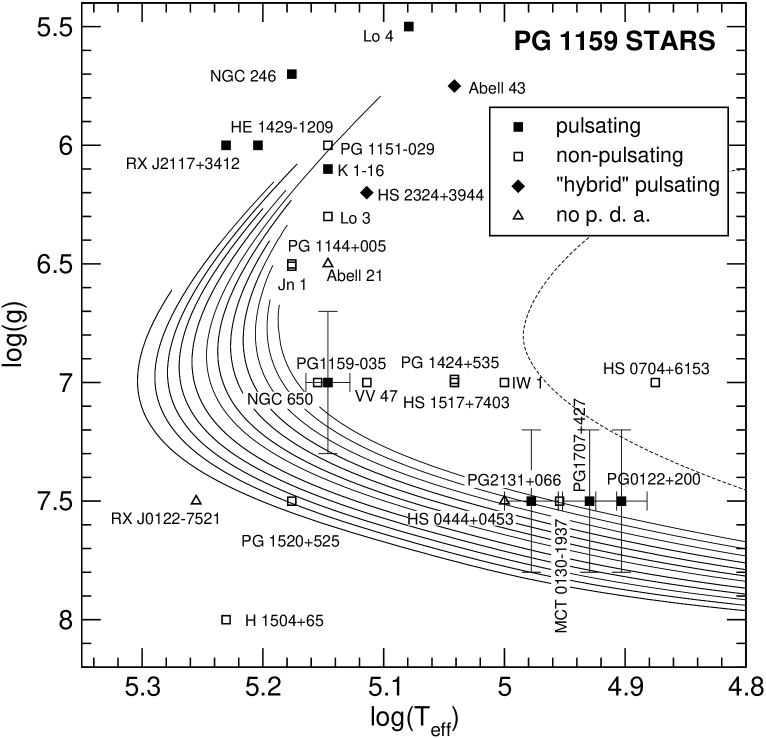
Figure 1: The observed location of PG 1159 stars in the $\log T_{\rm eff}-\log g$ plane. Filled squares represent GW Vir pulsators, hollow squares represent non-pulsators PG 1159 stars, diamonds correspond to “hybrid-PG 1159” stars and triangles represent stars with no photometric data available. Data are taken from Kawaler et al. (2004), Werner et al. (1997), Dreizler & Heber (1998), Nagel & Werner (2004), and Vauclair et al. (2005). PG 1159 evolutionary tracks — this work; see also Althaus et al. (2005) — are indicated with solid curves; stellar masses are from right to left $0.53,0.54,\ldots,0.64M_{\odot}$. Dashed curve corresponds to an AGB-manquè evolutionary track of a model star with $M_{*}=0.49M_{\odot}$ (Scóccola et al. 2005). In this and the remainig figures displaying results from our additional evolutionary sequences with different stellar masses, only results for evolutionary stages after the transitory phase has long vanished are shown (see text toward the end of §2).

GW Vir variables are low-amplitude, multiperiodic $g$-mode pulsators, with periods in the range from 5 to 30 minutes. Eleven of such variables are presently known, six of which associated with a planetary nebula and sometimes termed PNNV (Planetary Nebula Nuclei Variable). The remainder objects, lacking a surrounding nebulae, are called “naked” GW Vir stars. In Fig. 1 we plot the observed location of the known GW Vir stars in the $\log T_{\rm eff}-\log g$ plane. In addition, we have included in the figure some non-variable PG 1159 stars as well as PG 1159 stars for which photometric data are not available. Note that GW Vir stars are separated into two subgroups, one containing low-gravity, high-luminosity stars — the PNNVs RXJ2117+3412, HE1429-1209, K1-16, NGC 246, HS2324+3944, Lo 4 and Abell 43 —, and the other corresponding to high-gravity stars — the naked GW Vir stars PG 1159-035, PG 2131+066, PG 1707+427 and PG 0122+200. Finally, we note that among the low-gravity GW Vir stars there are two objects labeled as pulsating “hybrid-PG 1159” — HS2324+3944 and Abell 43. They are variable PG 1159 stars showing strong Balmer lines of hydrogen in their spectra.

A longstanding problem associated with GW Vir stars is related to the excitation mechanism for the pulsations and, in particular, to the chemical composition of the driving zone, an issue that has always attracted the attention of the theorists but that until very recently has eluded all the attempts of understanding. In their pioneering works, Starrfield et al. (1983, 1984, 1985) and Stanghellini et al. (1991) realized that $g$-mode pulsations with periods around 500 s could be driven in PG 1159 models by the $\kappa$-mechanism associated with the partial ionization of carbon and oxygen. While these authors were successful in finding the correct destabilizing mechanism, the periods of the excited modes were too short as compared with the observed periodicities in GW Vir stars. In addition, their models required a driving region very poor in helium in order to be capable to excite pulsations. The latter requirement led to the suspicion that a composition gradient would exist to make compatible the helium-devoid envelope and the helium-rich atmospheric layers. Even very recent theoretical work by Bradley & Dziembowski (1996) and Cox (2003) points out the necessity of a chemical composition in the driving region different from the observed surface composition. This is difficult to explain in view of the fact that PG 1159 stars are still experiencing mass loss, a fact that prevents the action of gravitational settling of carbon and oxygen. Clearly at odds with conclusions of these works, the calculations by Saio (1996) and Gautschy (1997), and more recently by Quirion et al. (2004) and Gautschy et al. (2005), demonstrate that $g$-mode pulsations in the range of periods of GW Vir stars could be easily driven in PG 1159 models at satisfactory effective temperatures with an uniform envelope composition compatible with the observed photospheric abundances.

While non-adiabatic stability issues like those mentioned above are of utmost importance in elucidating the cause of GW Vir pulsations and to place constraints on the composition of the subphotospheric layers, there is other avenue that may help to extract valuable information about the internal structure and evolutionary status of PG 1159 stars, by considering adiabatic pulsation periods alone. This approach, known as asteroseismology, allows us to derive structural parameters of individuals pulsators by matching adiabatic periods with the observed periodicities. Current examples of asteroseismic studies of GW Vir stars are those of Kawaler & Bradley (1994) (PG 1159-035), Kawaler et al. (1995) (PG 2131+066), O’Brien et al. (1998) (PG 0122+200), Vauclair et al. (2002) (RXJ2117+341) and Kawaler et al. (2004) (PG 1707+427). These studies have been successful in providing precise mass determinations and valuable constraints on the outer compositional stratification of PG 1159 stars. As important as they were, these investigations were based on stellar models that were not actually fully self-consistent evolutionary PG 1159 models. In addition, with the notable exception of the exemplary work of Kawaler & Bradley (1994), all these studies used the observed mean period spacing and the asymptotic theory of stellar pulsations alone to make asteroseismic inferences; that is, no detailed period fitting were carried out in those works. In part, the reason for this is that for most of GW Vir stars (with exception of PG 1159-035) the observed mode density appear to be not high enough for detailed asteroseismic analysis.

It is important to mention that for applications requiring accurate values of the adiabatic pulsation periods of GW Vir stars only full evolutionary models can be used. This is particularly true for asteroseismic fits to individual stars. In fact, as it has been shown, stellar models representing PG 1159 stars should reflect the thermal structure of their progenitors because is that structure which primarily determines the adiabatic period spectrum, at least at the high luminosity phases (Kawaler et al. 1985). This is of utmost importance concerning the theoretically expected rates of the pulsation period change — see, e.g., Kawaler et al. (1986). In addition, special care must be taken in the numerical simulations of the evolutionary stages prior to the AGB phase. Specifically, the modeling process should include extra mixing episodes beyond the fully convective core during central helium burning (Straniero et al. 2003). In particular, overshoot during the central helium burning stage leads to sharp variations of the chemical profile at the inner core — see Straniero et al. (2003); Althaus et al. (2003). This, in turn, could have a strong impact on the mode-trapping properties of the PG 1159 models. Last but not least, a self-consistent treatment of the post-AGB evolution is required. In fact, the details of the last helium thermal pulse on the early WD cooling branch and the subsequent born-again episode determines, to a great extent, the chemical stratification and composition of the outer layers of the hot PG 1159 stars. The composition stratification of the stellar envelope, in turn, plays an important role in the mode-trapping characteristics of PG 1159 stars — see Kawaler & Bradley (1994).

All these requirements are completely fulfilled by the 0.5895-$M_{\odot}$  PG 1159 models presented recently by Althaus et al. (2005). In fact, these authors have computed the evolution of hydrogen-deficient post-AGB WDs taking into account a complete and detailed treatment of the physical processes that lead to the formation of such stars. These models have been recently used for non-adiabatic studies of GW Vir stars by Gautschy et al. (2005). The aim of this paper is to explore the adiabatic pulsation properties of GW Vir stars by employing the full evolutionary PG 1159 models of Althaus et al. (2005). In addition, we employ these models to make seismic inferences on several GW Vir stars. The paper is organized as follows. In Sect. 2, we describe the main characteristics of our numerical codes and the PG 1159 models employed. The adiabatic pulsational properties for our PG 1159 sequences are described in detail in §3. Special emphasis is given to the mode-trapping properties of our models. Sect. 4 is devoted to describing the application of our extensive period computations for asteroseismic inferences of the main structural properties of various high-gravity GW Vir stars. Finally, in §5 we briefly summarize our main findings and draw our conclusions.

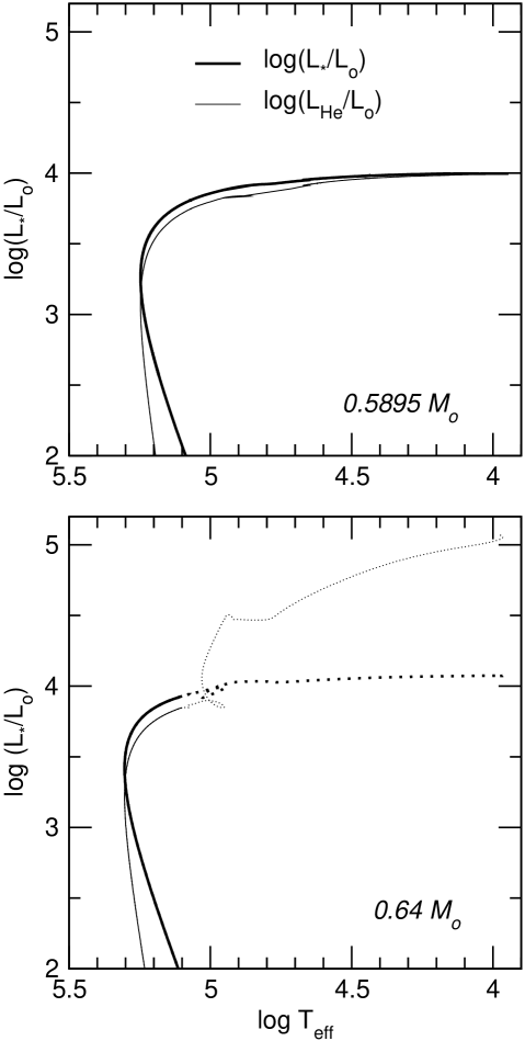
Figure 2: The surface (thick line) and helium-burning (thin line) luminosities ($\log L_{*}/L_{\odot}$ and $\log L_{\rm He}/L_{\odot}$, respectively) in terms of the effective temperature. The upper panel depicts the situation for our consistent 0.5895-$M_{\odot}$  sequence. The bottom panel corresponds to the 0.64-$M_{\odot}$  artificially generated sequence, in which the the unphysical evolutionary stages are indicated with dotted lines. For details, see text.

2 Evolutionary code, input physics and stellar models for GW Vir stars

The adiabatic pulsational analysis presented in this work is based on artificial PG1159 evolutionary sequences with different stellar massess. These sequences have been derived from a full post-born again evolutionary sequence of 0.5895 $M_{\odot}$  (Althaus et al. 2005) that has been computed taking into account the evolutionary history of the progenitor star. Specifically, the evolution of an initially $2.7\,M_{\sun}$ stellar model from the zero-age main sequence has been followed all the way from the stages of hydrogen and helium burning in the core up to the tip of the AGB where helium thermal pulses occur. We mention that during the thermally pulsing AGB phase our models experience appreciable third dredge-up which causes the carbon-oxygen ratio to increase from $\approx 0.25$ to $\approx 0.34$ by the time the remnant departs from the AGB. Apart from implications for the chemical stratification of the post-AGB remnant, the occurrence of the third dredge-up mixing event affects the degeneracy of the carbon-oxygen core, which in turn affects the location of the PG1159 tracks (see Werner & Herwig 2006 for comments). After experiencing 10 thermal pulses, the progenitor departs from the AGB and evolves toward high effective temperatures, where it experiences a final thermal pulse during the early WD cooling phase — a very late thermal pulse and the ensuing born-again episode, see Blöcker (2001) for a review — where most of the residual hydrogen envelope is burnt. After the occurrence of a double-loop in the Hertzsprung-Russell diagram, the now hydrogen-deficient, quiescent helium-burning 0.5895-$M_{\odot}$remnant evolves at almost constant luminosity to the domain of PG 1159 stars with a surface chemical composition rich in helium, carbon and oxygen: (⁴He,¹²C,¹⁶O)= (0.306, 0.376, 0.228). This is in good agreement with surface abundance patterns observed in pulsating PG 1159 stars (Dreizler & Heber 1998; Werner 2001). Also, the surface nitrogen abundance (about 0.01 by mass) predicted by our models is in line with that detected in pulsating PG 1159 stars (see Dreizler & Heber 1998).

We mention that the nuclear network considered in the stellar modelling accounts explicitly for 16 chemical elements and 34 thermonuclear reaction rates to describe hydrogen and helium burning. Abundances changes for the elements considered was included by means of a time-dependent scheme that simultaneously treats nuclear evolution and mixing processes due to convection and overshooting. A treatment of this kind is particularly necessary during the extremely short-lived phase of the born-again episode, for which the assumption of instantaneous mixing is inadequate. In particular, overshooting is treated as a diffusion process (see, e.g., Herwig et al. 1997) and has been considered during all evolutionary phases. Radiative opacities are those of OPAL (including carbon- and oxygen-rich compositions; Iglesias & Rogers 1996), complemented, at low temperatures, with the molecular opacities from Alexander & Ferguson (1994).

Because of the considerable load of computing time and numerical difficulty issues involved in the generation of PG 1159 stellar models that take into account the complete evolutionary history of the progenitor star, we were forced to consider one case for the complete evolution, that is, the 0.5895-$M_{\odot}$  sequence. However, to reach a deeper understanding of the various trends exhibited by pulsations in GW Vir stars, an assessment of the dependence of the pulsation properties of PG1159 models with the several structural parameters should be highly desirable. This statement is particularly true regarding the stellar mass of the models. In this paper we consider a set of additional sequences of models within a small range of stellar masses. In absence of actual self-consistent evolutionary computations of post-born again PG1159 models with different stellar masses, we elect to create several evolutionary sequences by employing an artificial procedure starting from our “seed” model sequence of 0.5895 $M_{\odot}$(see below). This approach has been adopted in many pulsation studies aimed at exploring the effects of different model parameters on the pulsation properties (see, e.g., Kawaler & Bradley 1994), starting from a post-AGB evolutionary model. At variance with previous calculations, in this work we derived additional model sequences with stellar masses in the ranges $0.53-0.58$ $M_{\odot}$  and $0.60-0.64$ $M_{\odot}$  (with a step of 0.01 $M_{\odot}$ ) from the post-born again 0.5895-$M_{\odot}$  sequence previously described. To this end, we artificially changed the stellar mass to the appropriate values shortly after the end of the born-again episode. Although this procedure led to a sequence of unphysical stellar models for which the helium-burning luminosity is not consistent with the thermo-mechanical structure of the models, we found that the transitory stage vanishes at high luminosities, before the star reaches the “knee” in the $\log T_{\rm eff}-\log g$ plane This can be understood by examining Fig. 2 which shows the surface and helium-burning luminosities in terms of the effective temperature. The upper panel depicts the situation for our consistent 0.5895-$M_{\odot}$  sequence. The bottom panel corresponds to the 0.64-$M_{\odot}$  artificially generated sequence. Note that, as result of the change in the thermal structure of the outer layers induced by the abrupt change in the stellar mass (at low effective temperatures), the helium-burning luminosity becomes seriously affected. Note that once the transitory stage has disappeared, the helium-burning luminosity follows a similar trend to that expected from the full evolutionary computation (upper panel). In the bottom panel, the unphysical evolutionary stages are indicated with dotted lines, while the solid lines correspond to the evolutionary stages which we consider valid for the purposes of this paper. Thus, the tracks depicted in Fig. 1 correspond to those stages of the evolutionary sequences for which the unphysical transitory has long disappeared. We stress that pulsation results presented along this work will be performed on stellar models belonging to the evolutionary sequences shown in Fig. 1 (see also Fig. 3). We warn again that the pulsational results presented here are based on stellar models artificially constructed, and that full evolutionary models with different stellar masses and complete evolutionary history are required to place such results on a solid background.

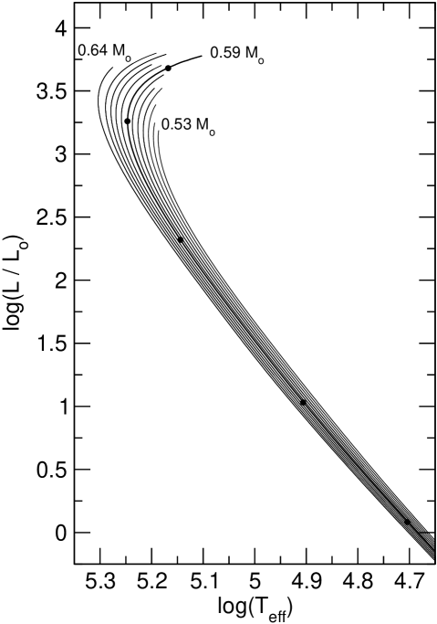
Figure 3: Evolutionary tracks for sequences with stellar masses, from right to left, of $0.53,0.54,\ldots,0.64M_{\odot}$. The sequence with $0.5895M_{\odot}$ is indicated with thicker line. For this sequence, the black dots mark the location of five specific models to be analyzed in §3.2.

We stress that, since we do not account for the complete evolution of the progenitor stars (except for the 0.5895-$M_{\odot}$  sequence), the internal composition of the models we use in part of our pulsational analysis may not be completely realistic, a fact that should be kept in mind when we analyze, in particular, the dependence of the asymptotic period spacing and mode trapping properties with the stellar mass. We also stress that the shape of the carbon/oxygen profile — particularly in the core — is quite sensitive to the adopted reaction rates during the central helium burning phase (see Kunz et al. 2002; Straniero et al. 2003) and the efficiency of the convection-induced mixing (overshooting and/or semiconvection; see Straniero et al. 2003). In particular, we have recently found (Córsico & Althaus 2005) that with a lower rate of the ¹²C$(\alpha,\gamma)^{16}$O reaction than we adopted here, the central abundances of oxygen and carbon become quite similar, partially smoothing the chemical steps in the core. However, as shown in that paper, the mode trapping structure resulting from the core is not seriously altered.

3 Adiabatic pulsational analysis

In this section we present an extensive adiabatic analysis of our grid of PG 1159 evolutionary models. Since the most detailed and thorough reference in the literature on adiabatic pulsations of PG 1159 stars is the work of Kawaler & Bradley (1994) [hereinafter KB94], we shall invoke repeatedly that paper throughout this work to compare their results with our own findings. We have assessed the pulsation properties of about 3000 stellar models, the stellar mass of which range from 0.53 $M_{\odot}$ to 0.64 $M_{\odot}$, embracing the well-established mean mass for WDs. Fig. 3 shows the evolutionary tracks of our model sequences. All of our PG 1159 sequences are characterized by a helium layer thickness of $0.0052M_{\odot}$ — as predicted by our evolutionary calculations for the 0.5895-$M_{\odot}$ models (Althaus et al. 2005). For each analyzed model we have computed $g$-mode periods in the range $50-2500$ s, although in some cases we have extended the range of periods and also included $p$-mode computations. We limited our calculations to the degrees $\ell=1,2$ because the periods observed in pulsating PG 1159 stars have been positively identified with $\ell=1,2$ (see, e.g., Winget et al 1991; Vauclair et al. 2002). Since one of the purposes of this work is to get values of adiabatic periods as precise as possible, we have employed about $2700-3000$ mesh-points to describe our background stellar models.

3.1 Pulsation code and adiabatic quantities

We begin this section with a brief description of the pulsation code employed and the relevant pulsation quantities. For computing pulsation modes of our PG 1159 models we use an updated version of the pulsational code employed in Córsico et al. (2001). Briefly, the code, which is coupled to the LPCODE evolutionary code, is based on the general Newton-Raphson technique and solves the full fourth-order set of equations governing linear, adiabatic, nonradial stellar pulsations following the dimensionless formulation of Dziembowski (1971). The pulsation code provides the dimensionless eigenfrequency $\omega_{k}$ — $k$ being the radial order of the mode — and eigenfunctions $y_{1},\cdots,y_{4}$. From these basic quantities the code computes the pulsation periods ($\Pi_{k}$), the oscillation kinetic energy ($K_{k}$), rotation splitting coefficients ($C_{k}$), weight functions ($W_{k}$), and variational periods ($\Pi_{k}^{\rm v}$) for each computed eigenmode. Usually, the relative difference between $\Pi_{k}^{\rm v}$ and $\Pi_{k}$ is lower than $\approx 10^{-4}$. The pulsation equations, boundary conditions and relevant adiabatic quantities are given in Appendix A.

The prescription we follow to assess the run of the Brunt-Väisälä frequency ($N$) is the so-called “Ledoux Modified” treatment — see Tassoul et al. (1990) — appropriately generalized to include the effects of having three nuclear species (oxygen, carbon and helium) varying in abundance (see KB94). In this numerical treatment the contribution to $N$ from any change in composition is almost completely contained in the Ledoux term $B$; this fact renders the method particularly useful to infer the relative weight that each chemical transition region have on the mode-trapping properties of the model (see §3.4). Specifically, the Brunt-Väisälä frequency is computed as:

$$N^{2}=\frac{g^{2}\ \rho}{p}\ \frac{\chi_{\rm T}}{\chi_{\rho}}\ \left(\nabla_{\rm ad}-\nabla+B\right)$$ (1)

where

$$B=-\frac{1}{\chi_{\rm T}}\sum^{n-1}_{i=1}\chi_{{\rm X}_{i}}\frac{d\ln X_{i}}{d\ln p},$$ (2)

being

$$\chi_{\rm T}=\left[\frac{\partial\ln{p}}{\partial\ln{T}}\right]_{\rho}\ \ \chi_{\rm\rho}=\left[\frac{\partial\ln{p}}{\partial\ln{\rho}}\right]_{T}\ \ \chi_{{\rm X}_{i}}=\left[\frac{\partial\ln{p}}{\partial\ln{X_{i}}}\right]_{\rho,T,{X_{j\neq i}}}$$ (3)

Fig. 4 shows a representative spatial run of the Brunt-Väisälä frequency for a PG 1159 model. The model is characterized by a stellar mass of $0.5895$ $M_{\odot}$, an effective temperature of $\approx 139\,000$ K and a luminosity of $\log(L_{*}/L_{\odot})=2.31$. In addition, the plot shows the internal chemical stratification of the model for the main nuclear species (upper region of the plot) and for illustrative purposes the profile of the Ledoux term $B$ (inset). The figure emphasizes the role of the chemical interfaces on the shape of the Brunt-Väisälä frequency. In fact, each chemical transition region produces clear and distinctive features in $N$, which are eventually responsible for the mode-trapping properties of the model. At the core region there are several peaks at $M_{r}/M_{*}\approx 0.4-0.6$ resulting from steep variations in the inner oxygen/carbon profile. The stepped shape of the carbon and oxygen abundance distribution within the core is typical for situations in which extra mixing episodes beyond the fully convective core during central helium burning are allowed. In particular, the sharp variation around $M_{r}\approx 0.56M_{*}$, which is left by overshoot at the boundary of the convective core during the central helium burning phase, could be a potential source of mode-trapping in the core region — “core-trapped” modes; see Althaus et al. (2003) in the context of massive DA WD models. The extended bump in $N$ at $M_{r}\approx 0.96M_{*}$ is other possible source of mode-trapping, in this case associated with modes trapped in the outer layers. This feature is caused by the chemical transition of helium, carbon and oxygen resulting from nuclear processing in prior AGB and post-AGB stages. In a subsequent Section we shall explore in detail the role played by the chemical transition regions on the mode-trapping properties of our PG 1159 evolutionary models.

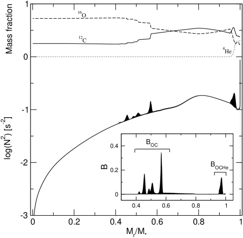
Figure 4: The run of the squared Brunt-Väisälä frequency in terms of the mass coordinate, corresponding to a $0.5895$-$M_{\odot}$PG 1159 model at $T_{\rm eff}=139\,000$ K and $\log(L_{*}/L_{\odot})=2.31$. The mass of the helium content is of $0.008821M_{*}$ ($0.0052M_{\odot}$). Dark regions denote the contributions of the Ledoux term $B$ (shown in the inset) to the Brunt-Väisälä frequency. The chemical profile is displayed in the upper zone of the plot.

3.2 The basic nature of the nonradial pulsation spectrum

This section is devoted to exploring at some length the basic properties of nonradial pulsation modes of our PG 1159 pre-WD evolutionary models. To this end, we have extended the scope of our pulsation calculations by including low order $g$-modes and also nonradial $p$-modes in the discussion, although we are aware that short periods like those associated with such modes have not been ever detected in variable PG 1159 stars. Here, we have chosen to analyze the sequence of $0.5895M_{\odot}$-models from the early phases of evolution at constant luminosity — shortly before the maximum of effective temperature — until the beginning of the WD cooling track — when models evolve at roughly constant radius. We stress that this is the first time that the adiabatic pulsation properties of fully evolutionary post born-again PG 1159 models are assessed — an exception is the non-adiabatic analysis of Gautschy et al. (2005). Thus, we believe that it is instructive to look into the basic features of the full nonradial pulsation spectrum of these models.

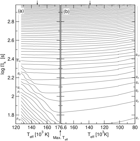
Figure 5: The evolution of the $\ell=1$ pulsation periods $\Pi_{k}$ in terms of the effective temperature, corresponding to the sequence of $0.5895M_{\odot}$-models. Panel (a) depicts the situation before the models reach the maximum value of effective temperature (Max. $T_{\rm eff}$), and panel (b) shows the situation when the models have already passed through this stage. Arrows indicate the effective temperature corresponding to two elected models that are analyzed in Figs. 6 and 7. Note that the orientation of the $T_{\rm eff}$ axis in panel (a) is opposite to that of panel (b). See text for details.

We begin by describing the evolution of the period spectrum. For the $0.5895M_{\odot}$ sequence we have available physically meaningful stellar models from stages previous to the beginning of the WD cooling track. This fact allows us to perform an exploratory exercise of the period spectrum from the moment when the objects still retain the thermal structure resulting from prior evolution of the progenitor star. In Fig. 5 we show the $\ell=1$ pulsation periods $\Pi_{k}$ in terms of the effective temperature before (panel a) and after (panel b) the model reach the turning point in the H-R diagram (see Fig. 3). We find the pulsation periods to decrease in stages in which the model is still approaching to its maximum effective temperature ($T_{\rm eff}\approx 176\,600$ K). This is because the star is undergoing a rapid contraction, in particular at the outer layers. As is well known, contraction effects lead to a decrease in the pulsation periods (see Winget et al. 1983). When the model has already settled into their cooling phase, the periods increase in response to the decrease of the Brunt-Väisälä frequency. Thus, the behavior exhibited is typical of WD pulsators, with increasing periods as the effective temperature decreases. Note in panel (a) of Fig. 5 that when $T_{\rm eff}<176\,600$ K, the low order periods ($\Pi_{k}\lesssim 200$ s) exhibit a behavior reminiscent to the well known “avoided crossing”. When a pair of modes experiences avoided crossing, the modes exchange their intrinsic properties (see Aizenman et al. 1977). As we shall see below, these are modes with a mixed character, that is, modes that behave as $g$-modes in certain zones of the star and as $p$-modes in other regions.

In order to obtain valuable qualitative information of nonradial pulsations we apply a local treatment to the pulsation equations (Unno et al. 1989). Employing the Cowling approximation, in which the perturbation of the gravitational potential is neglected ($\Phi^{\prime}=0$), and assuming that the coefficients of the pulsation equations are almost constant — that is, in the limit of high radial order $k$ — we obtain simple expressions for the eigenfunctions: $y_{1},y_{2}\propto\exp(ik_{r}r)$, and an useful dispersion relation follows: $k_{r}^{2}=\sigma^{-2}c^{-2}\left(\sigma^{2}-N^{2}\right)\left(\sigma^{2}-L_{\ell}^{2}\right)$, which relates the local radial wave number $k_{r}$ to the pulsation frequency $\sigma$. $L_{\ell}$ is the Lamb frequency, defined as $L_{\ell}^{2}=\ell(\ell+1)c^{2}/r^{2}$. Note that if $\sigma^{2}>N^{2},L_{\ell}^{2}$ or $\sigma^{2}<N^{2},L_{\ell}^{2}$, the wave number $k_{r}$ is real, and if $N^{2}>\sigma^{2}>L_{\ell}^{2}$ or $N^{2}<\sigma^{2}<L_{\ell}^{2}$, $k_{r}$ is purely imaginary.

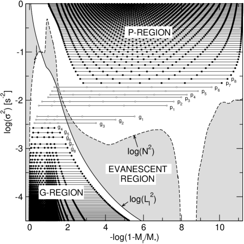
Figure 6: Propagation diagram corresponding to a PG 1159 evolutionary model characterized by $[M_{*}/M_{\odot},\log(L_{*}/L_{\odot}),\log T_{\rm eff}]=[0.5895,3.68,5.168]$ for $\ell=1$ modes. The effective temperature of this model is marked with an arrow in panel (a) of Fig. 5. White (gray) areas correspond to propagation (evanescent) zones according the local analysis described in the text. The square of the Brunt-Väisälä frequency ($N$) and the Lamb frequency ($L_{\ell}$) are depicted with dashed and solid lines, respectively. Horizontal thin lines show the square of the eigenfrequencies, and small symbols show the loci of the nodes of the radial eigenfunction, $y_{1}$ (filled circles: $g$-modes; filled squares: $p$-modes). Open circles correspond to nodes of modes with mixed character. These modes propagate in both P- and G-regions. Note the excellent agreement between the full numerical solution and the predictions of the simple local treatment.

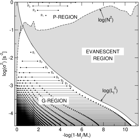
Figure 7: Same of Fig. 6, but for a PG 1159 model characterized by $[M_{*}/M_{\odot},\log(L_{*}/L_{\odot}),\log T_{\rm eff}]=[0.5895,2.31,5.143]$. The effective temperature of the model is that marked with an arrow in panel (b) of Fig. 5. Note that in this case the G and P branches of modes are clearly separated in frequency.

In Fig. 6 we show $L_{\ell}^{2}$ and $N^{2}$ as functions of $-\log(1-M_{r}/m_{*})$. This type of diagrams are called propagation diagrams (see, e.g., Unno et al. 1989; Cox 1980). The figure corresponds to a PG 1159 model with $M_{*}=0.5895M_{\odot}$, $\log(L_{*}/L_{\odot})=3.68$ and $T_{\rm eff}=147\,200$ K. This model corresponds to a stage in which the star is still approaching to its maximum $T_{\rm eff}$ (see the arrow in panel (a) of Fig. 5). The dashed curve shows the square of the Brunt-Väisälä frequency, and the solid curve depicts the run of the square of the Lamb frequency for $\ell=1$. Since this model still retains some similarities to those of the red giants from which these models are descendants, the Brunt-Väisälä frequency is characterized by large central values as compared to those characterizing the outer regions. In the plot, gray areas correspond to regions in which $k_{r}$ is purely imaginary. As a result, modes should be unable to propagate in these “evanescent” zones. In contrast, in regions in which $k_{r}$ is real (white areas in the plot) modes should be oscillatory in space, and these regions correspond to “propagation” zones. As we can see in the figure, there exist two propagation regions, one corresponding to the case $\sigma^{2}>N^{2},L_{\ell}^{2}$, associated with $p$-modes (P-region), and other in which the eigenfrequencies satisfies $\sigma^{2}<N^{2},L_{\ell}^{2}$, associated with $g$-modes (G-region). The predictions of this simple local analysis are nicely confirmed by our full numerical solution. Indeed, the figure shows the computed eigenfrecuencies of $p$- and $g$-modes (thin horizontal lines) and the loci of the nodes of the radial eigenfunction, $y_{1}$ (small symbols). Note that no node lies in the evanescent regions, meaning that the radial eigenfunction is not oscillatory here. This figure clearly shows that the $p$-modes and $g$-modes are trapped in the P-region and the G-region, respectively.

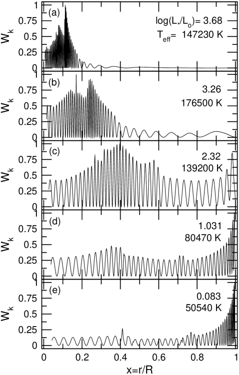
Figure 8: The normalized weight function of the mode $g_{40}$ vs the stellar radius corresponding to $0.5895M_{\odot}$-models at different effective temperatures. The location of the stellar models in the H-R diagram is shown in Fig. 3. Note that the regions in which $W_{k}$ adopts appreciable amplitude — the regions of period formation — move from the core toward the surface of the model.

Note that, because the very peculiar shape of the Brunt-Väisälä frequency in the inner regions of the star, there is a considerable range of intermediate frequencies in which the inner parts of the star lie predominantly in the G-region, and the outer parts lie in the P-region. Thus, these intermediate-frequency modes possess a mixed character: they behave like $g$-modes in the inner parts of the star and like $p$-modes in the outer parts. In Fig. 6 these modes are indicated with open circles. Note that nodes in $y_{1}$ for such modes may occur in both the P- and G-regions. In order to get the radial order of these modes we employ the scheme of Scuflaire (1974). In the figure modes with mixed character and some low order “pure” $p$- and $g$-modes are appropriately labeled.

Fig. 7 shows a propagation diagram corresponding to a model characterized by $M_{*}=0.5895M_{\odot}$, $\log(L_{*}/L_{\odot})=2.31$ and $T_{\rm eff}=139\,000$ K. Unlike the model described in Fig. 6, this PG 1159 model is already located at the early WD cooling track — its effective temperature is marked with an arrow in panel (b) of Fig. 5. We expect that the fundamental properties of its pulsational spectrum should be reminiscent to that of the pulsating WD stars. In fact, the Brunt-Väisälä frequency shows larger values in the outer regions than in the core, in such a way that the propagation regions P and G are markedly separated. As a result, modes with mixed character no longer exist, and the families of $g$- and $p$-modes are clearly differentiated. In this case, the radial order of the modes is simply the number of the nodes of the radial eigenfunction. Note that for this model the $g$-modes are free to propagate throughout the star, at variance with the situation of the model described in Fig. 6, in which $g$-modes are strongly confined to the core region.

The regions of the star that most contribute to the period formation are inferred from Fig. 8, which shows the normalized weight function (Eq. (19) of the Appendix) of a $g$-mode with $k=40,\ell=1$ in terms of the stellar radius corresponding to $0.5895M_{\odot}$-models at different effective temperatures. The location of these models in the H-R diagram is depicted as black dots in Fig. 3. Note that, for the model at $T_{\rm eff}\approx 147\,000$ K (panel a), $W_{k}$ adopts appreciable amplitudes only in central regions. Since the behavior of the weight function for this mode is representative of all $g$-modes with intermediate and high radial order $k$, we conclude that the $g$-mode pulsation periods for PG 1159 models that have not still reached the maximum in $T_{\rm eff}$ are mostly determined by the core regions of the star, irrespective of the structure of the outer layers. Thus, for models at high-luminosity phases the adiabatic pulsations properties reflect the conditions in the degenerate core. The situation for a model placed exactly at the turning point in $T_{\rm eff}$ is depicted in panel (b) of Fig. 5, corresponding to $T_{\rm eff}=176\,500$ K and $\log(L_{*}/L_{\odot})=3.26$. Note that, at this stage, the regions of period formation have extended towards more external zones. By the time the model has settled into its WD cooling track, the weight function exhibits appreciable values throughout the star, having some amplitude also in the outer regions, as displayed in panel (c). Below $\sim 100\,000$ K, the weight function adopts its maximum value in the outer layers, as can be seen in panels (d) and (e). At these stages, the adiabatic periods are mainly determined by the outer envelope, although the inner regions of the star also contribute to establishing the period of oscillation. Our findings are in full agreement with the results of the early computations of Kawaler et al. (1985) — for instance, compare our Fig. 8 with their figure 5.

3.3 Asymptotic period spacing

In the asymptotic limit of very high radial order $k$ (long periods), the periods of $g$-modes of a chemically homogeneous stellar model for a given degree $\ell$ and consecutive $k$ are separated by a constant period spacing $\Delta\Pi_{\ell}^{\rm a}$, given by (Tassoul et al. 1990):

$$\Delta\Pi_{\ell}^{\rm a}=\frac{\Pi_{0}}{\sqrt{\ell(\ell+1)}}=\frac{2\pi^{2}}{\sqrt{\ell(\ell+1)}}\left[\int_{x_{1}}^{x_{2}}\frac{N}{x}dx\right]^{-1}.$$ (4)

Note that $\Pi_{0}$ (and $\Delta\Pi_{\ell}^{\rm a}$) is a function of the structural properties of the star through the Brunt-Väisälä frequency. The integral is taken over the $g$-mode propagation region. While for chemically homogeneous models the asymptotic formula (4) constitutes a very precise description of their pulsational properties, the computed $g$-mode period spacings ($\Delta\Pi_{k}\equiv\Pi_{k+1}-\Pi_{k}$) in chemically stratified PG 1159 models show appreciable departures from uniformity caused by mode trapping (see next Section). However, the average of the computed period spacings $\overline{\Delta\Pi_{k}}$ is very close to the asymptotic period spacing $\Delta\Pi_{\ell}^{\rm a}$ when averaged over several modes.

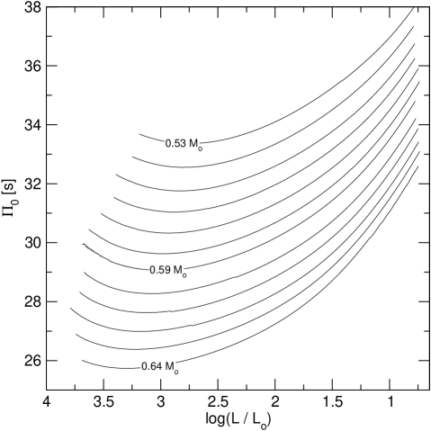
Figure 9: The evolution of $\Pi_{0}$ in terms of stellar luminosity for evolutionary models of different stellar masses ($0.53,\cdots,0.64M_{\odot}$ from top to bottom). As in Figs. 1 and 3, only results corresponding to models whose structure has completely forgotten the unphysical transitory stage (after we switch the stellar mass value; see toward the end of Sect. 2) are shown.

The evolution of $\Pi_{0}$ vs the stellar luminosity for models with different stellar masses is displayed in Fig. 9. In line with previous works (see, e.g., KB94), our results indicate that $\Pi_{0}$ increases with decreasing stellar mass. In particular, the value of $\Pi_{0}$ exhibits an increment of about $6-8$ s when the stellar mass decreases about $0.1M_{\odot}$. This is due to the fact that the asymptotic period spacing is inversely proportional to the integral of $N$ (Eq. 4). As we go to lower stellar masses, the Brunt-Väisälä frequency decreases and consequently $\Pi_{0}$ goes up.

Fig. 9 shows that $\Pi_{0}$ is also a function of the stellar luminosity, although the dependence is much weaker than the dependence on the stellar mass. As documented by the figure, for $\log(L_{*}/L_{\odot})\lesssim 3.25-2.75$ — depending on the stellar mass — the period spacing increases with decreasing the luminosity. This fact can be explained on the basis that, due to the increasing degeneracy in the core as the star cools, the Brunt-Väisälä frequency gradually decreases, causing a slow increment in the magnitude of $\Pi_{0}$. Finally, since in this work we do not consider different helium layer mass values, we have not been able to assess the possible dependence of the asymptotic period spacing on $M_{\rm He}$. However, this dependence is expected to be very weak (see KB94).

3.4 Mode-trapping properties

As we have mentioned before, the period spectrum of chemically homogeneous stellar models is characterized by a constant period separation, given very accurately by Eq. (4). However, current evolutionary calculations predicts that PG 1159 stars — as well as (hydrogen-rich) DA and (helium-rich) DB WD stars — must have composition gradients in their interiors, something that also the observation indicates. The presence of one or more narrow regions in which the abundances of nuclear species are rapidly varying strongly modifies the character of the resonant cavity in which modes should propagate as standing waves — the propagation region. Specifically, chemical interfaces act like reflecting boundaries that partially trap certain modes, forcing them to oscillate with larger amplitudes in specific regions — bounded either by two interfaces or by one interface and the stellar centre or surface — and with smaller amplitudes outside of that regions. The requirement for a mode to be trapped is that the wavelength of its radial eigenfunction matches with the spatial separation between two interfaces or between one interface and the stellar centre or surface. This mechanical resonance, known as mode trapping, has been the subject of intense study in the context of stratified DA and DB WD pulsations — see, e.g., Brassard et al. (1992); Bradley et al. (1993); Córsico et al. (2002). In the field of PG 1159 stars, mode trapping has been extensively explored by KB94; we refer the reader to that work for details.

There are (at least) two ways to identify trapped modes in a given stellar model. First, we can consider the oscillation kinetic energy, $K_{k}$. We stress that, because the amplitude of eigenfunctions is arbitrarily normalized at the model surface in our calculations (see the Appendix), the values of the kinetic energy are useful only in a relative sense. $K_{k}$ is proportional to the integral of the squared amplitude of eigenfunctions, weighted by the density (see Eq. 18 in the Appendix). Thus, modes propagating in the deep interior of the star, where densities are very high, will exhibit larger values than modes which are oscillating in the low-density, external regions. When only a single chemical interface is present, modes can be classified as modes trapped in the outer layers, modes confined in the core regions, or simply “normal modes” — which oscillate everywhere in the star — characterized by low, high, and intermediate $K_{k}$ values, respectively (see Brassard et al. 1992). This rather simple picture becomes markedly complex when the stellar model is characterized by several chemical composition gradients — see Córsico et al. (2002) for the case of ZZ Ceti models.

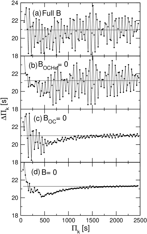
Figure 10: The forward period spacing $\Delta\Pi_{k}$ vs period $\Pi_{k}$ for dipole ($\ell=1$) modes. The asymptotic period spacing $\Delta\Pi_{\ell}^{\rm a}$ as given by Eq. (4) is depicted with a thin horizontal line. Panel (a) corresponds to the same PG 1159 model considered in Fig. 4. Remainder panels correspond to the same stellar model but for the situation in which the Ledoux term has been artificially suppressed in specific regions of the model: (b) $B=0$ at $M_{r}/M_{*}\approx 0.96$, (c) $B=0$ at $M_{r}/M_{*}\approx 0.4-0.6$, and (d) $B=0$ everywhere in the star.

A second — and more important from an observational point of view — consequence of mode trapping is that the period spacing $\Delta\Pi_{k}$, when plotted in terms of the pulsation period $\Pi_{k}$, exhibits strong departures from uniformity. It is the period difference between an observed mode and adjacent modes ($\Delta k=\pm 1$) that is the observational diagnostic of mode trapping — at variance with $K_{k}$, whose value is very difficult to estimate only from observation. For stellar models characterized by a single chemical interface, local minima in $\Delta\Pi_{k}$ usually correspond directly to modes trapped in the outer layers, whereas local maxima in $\Delta\Pi_{k}$ are associated to modes trapped in the core region.

We now turn out to the specific case of our PG 1159 pre-WD models. As Fig. 4 shows, they exhibit several chemical interfaces, some associated with the various steps in the ¹⁶O and ¹²C profile at the core region, and a single, more external transition region in which oxygen, carbon and helium are continuously varying (see Fig. 4). As stated in Sect. 3.1, these composition gradients produce pronounced peaks in the Brunt-Väisälä frequency — through the Ledoux term — that strongly disturb the structure of the period spectrum.

The influence of the chemical composition gradients inside our PG 1159 models on their period spectra is clearly shown in panel (a) of Fig. 10, in which the $\ell=1$ period spacing is plotted in terms of the periods for a reference model characterized by a stellar mass of $0.5895M_{\odot}$, an effective temperature of $139\,000$ K and a luminosity of $204.2L_{\odot}$. The plot shows very rapid variations of $\Delta\Pi_{k}$ everywhere in the period spectrum, with “trapping amplitudes” up to about 6 s and an asymptotic period spacing of $\approx 20.94$ s. The rather complex period-spacing diagram shown by Fig. 10 is typical of models characterized by several chemical interfaces. In order to isolate the effect of each chemical composition gradient on mode trapping, we follow the procedure of Charpinet et al. (2000) for models of sdB stars — see also Brassard et al. (1992) for the case of ZZ Ceti stars. Specifically, we minimize — although no completely eliminate — the effects of a given chemical interface simply by forcing the Ledoux term $B$ to be zero in the specific region of the star in which such interface is located. In this way, the resulting mode trapping will be only due to the remainder chemical interfaces. In the interest of clarity, we label as “$B_{\rm OCHe}$” the contribution to $B$ due to the O/C/He chemical interface at $M_{r}/M_{*}\approx 0.96$, and “$B_{\rm OC}$” the contribution to $B$ associated with the O/C chemical interface at $M_{r}/M_{*}\approx 0.4-0.6$ — see inset of Fig. 4. Specifically, we have recomputed the entire $g$-mode period spectrum under the following assumptions: (1) $B_{\rm OCHe}=0$ and $B_{\rm OC}\neq 0$, (2) $B_{\rm OCHe}\neq 0$ and $B_{\rm OC}=0$, and (3) $B_{\rm OCHe}=0$ and $B_{\rm OC}=0$ ($B=0$ in all regions). The results are shown in panels (b), (c) and (d) of Fig. 10, respectively. By comparing the different cases illustrated, an important conclusion emerges from this figure: the chemical transition region at $M_{r}\approx 0.96M_{*}$ is responsible for the non-uniformities in $\Delta\Pi_{k}$ only for $\Pi_{k}\lesssim 500$ s (panel c), whereas the chemical composition gradients at the core region ($M_{r}\approx 0.4-0.6M_{*}$) cause the mode-trapping structure in the rest of the period spectrum (panel b). When $B=0$ everywhere inside the model (panel d), the period-spacing diagram is characterized by the absence of strong features of mode trapping, although some structure remains, in particular for low order modes. Note the nice agreement between the numerical computations of $\Delta\Pi_{k}$ and the predictions of the asymptotic theory given by Eq. (4) for the limit $k\gg 1$.

From the above discussion, it is clear that the mode-trapping features characterizing our PG 1159 models are inflicted by the stepped shape of the carbon/oxygen chemical profile at the core — left by prior convective overshooting— at least for the range of periods observed in GW Vir stars. On their hand, the more external chemical transition has a minor influence, except for the regime of short periods. We mention that this situation is more evident for the more massive PG 1159 models than for the less massive ones.

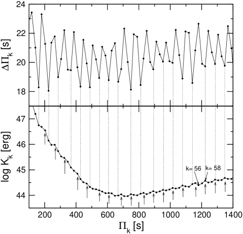
Figure 11: Period-spacing diagram and kinetic energy distribution (upper and lower panel, respectively) for the same PG 1159 model considered in panel (a) of Fig. 10. Vertical dotted lines link local minima in $\Delta\Pi_{k}$ with the corresponding values of $K_{k}$. Maximum values of kinetic energy are indicated with arrows. Also labeled are the modes with $k=56$ and $k=58$, to be analyzed in Fig. 12.

The findings outlined above are clearly at odd with previous results reported by KB94. Indeed, these authors have found that the mode-trapping properties of their PG 1159 models are fixed mainly by the outer O/C/He transition region, to a such a degree that they have been able to employ mode-trapping signatures as a sensitive locator of this transition region. The origin of this discrepancy can be found in the details of the input physics employed in build up the background stellar models. Of particular interest here is the presence of a much less pronounced chemical transition in the outer parts of the C/O core of the KB94 models, as compared with the rather abrupt chemical gradients at $M_{r}\approx 0.4-0.6M_{*}$ characterizing our PG 1159 models. If we artificially minimize the effect of this transition region — by setting $B_{\rm OC}=0$ — we immediately recover the results of KB94. Indeed, the period-spacing diagram of panel (c) in our Fig. 10 looks very similar to that shown in Fig. 3 of KB94, corresponding to $M_{\rm He}/M_{*}=0.00622$. We note, however, that the “trapping cycle” — the period interval between two period-spacing minima — of our modified model (c) is of $\approx 70$ s, whereas the value of the KB94 model is $\approx 95$ s. This difference is due mainly to the fact that our model has a more massive helium envelope ($M_{\rm He}/M_{*}=0.00881$) than that of KB94.

By means of a simple numerical experiment we have identified the main source of mode trapping as due to the step-like chemical transition region located at the core. We now return to panel (a) of Fig. 10, and note that there is a kind of “beating” which modulates the trapping amplitude. We also note that this striking feature (seen in all of our models) persists even in the case in which the effect of the O/C/He transition is artificially minimized, as it is illustrated in panel (b). We have found that the beating exhibited by the period-spacing distribution is due to the combined mode-trapping effects caused by the various steps in the O/C chemical profile in the core. In fact, by performing period computations in which only the largest peak of the Ledoux term at $M_{r}\approx 0.58M_{*}$ (see inset of Fig. 4) is considered, the beating effect virtually vanishes, and the trapping amplitude becomes nearly constant.

Finally, to understand in more detail the mode-trapping properties of our models, we resort to the kinetic energy of modes. In Fig. 11 we plot the period spacing and the kinetic energy distribution (upper and lower panel, respectively) for the same PG 1159 model considered in panel (a) of Fig. 10. We connect with dotted lines each minimum in $\Delta\Pi_{k}$ with their corresponding value of $K_{k}$. We note that in spite of the strong non-uniformities exhibited by $\Delta\Pi_{k}$, the $K_{k}$ values of adjacent modes seem to be not very different amongst them. However, a closer inspection of the figure reveals that in most of the cases a minimum in $\Delta\Pi_{k}$ corresponds to a local maximum in $K_{k}$. Our results strongly suggest that modes associated with minima in the period-spacing diagram usually correspond to maxima in the kinetic energy distribution. They should be modes characterized by relatively high amplitude of their eigenfunctions and weight functions in the high-density environment characterizing the stellar core.

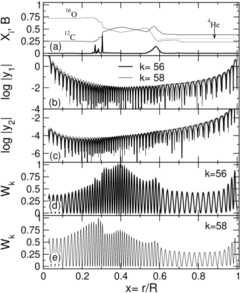
Figure 12: The spatial run of the modulus of the eigenfunctions $y_{1}$ and $y_{2}$, shown in panels (b) and (c), respectively, and the weight function $W_{k}$ depicted in panels (d) and (e), for dipole pulsation modes with $k=56$ (thick line) and $k=58$ (thin line) corresponding to the same PG 1159 model analyzed in Fig. 11. We also include in panel (a) the Ledoux term $B$ and the abundance (by mass) of ¹⁶O, ¹²C and ⁴He.

This is precisely what we have found after a careful examining of the eigenfunctions at the deepest regions of the core. In panels (b) and (c) of Fig. 12 we show the logarithm of the absolute value of the eigenfunctions $y_{1}$ and $y_{2}$ (see Eq. 13 of the Appendix for their definition), respectively, in terms of the dimensionless radius $x=r/R$, for a mode having a local maxima in kinetic energy ($k=58$, thin line) and for a mode having a local minima in $K_{k}$ ($k=56$, thick line). Note that below $r/R\approx 0.3$, the eigenfunctions of the $k=58$ mode have larger amplitudes than that of the $k=56$ mode, explaining why the $k=58$ mode has a relatively large oscillation kinetic energy. Modes like the $k=58$ one are partially trapped in the core region, below the O/C chemical interface (see panel a). As stated before, these modes correspond generally to minima in the period-spacing diagram. In panels (d) and (e) of Fig. 12 the normalized weight function ($W_{k}$) is displayed for the $k=56$ and $k=58$ modes, respectively. As we mentioned previously, the relative values of $W_{k}$ for a given pulsation mode provide information about the specific regions inside the star that most contribute to the period formation. From Fig. 12 we note that for the $k=58$ mode the maximum of $W_{k}$ is identified with the O/C chemical interface at $r/R\approx 0.3$, and the largest amplitude portion of the weight function is located in the deepest regions of the core ($r/R\lesssim 0.3$). For values of $r/R$ slightly larger than $0.3$, the weight function abruptly diminishes and then reaches a secondary maximum in the region in which ¹²C becomes more abundant than ¹⁶O. Above this region $W_{k}$ exhibit other secondary maximum at the O/C/He transition zone ($r/R\approx 0.58$), and above of this the weight function adopts rather lower values ($W_{k}\lesssim 0.3$). Thus, the shape of the weight function for the $k=58$ mode strongly suggests that the deepest regions of the core have the larger impact on the period formation of this mode. This conclusion is, not surprisingly, in complete agreement with the fact that this mode is characterized by a relatively high value of the oscillation kinetic energy. The situation is markedly different for the case of the $k=56$ mode, as it is clearly demonstrated by panel (d) of the figure. For this mode, most regions of the star appreciably contribute to the formation of its period. In particular, the most important contributions occur in regions located at $0.2\lesssim r/R\lesssim 0.6$.

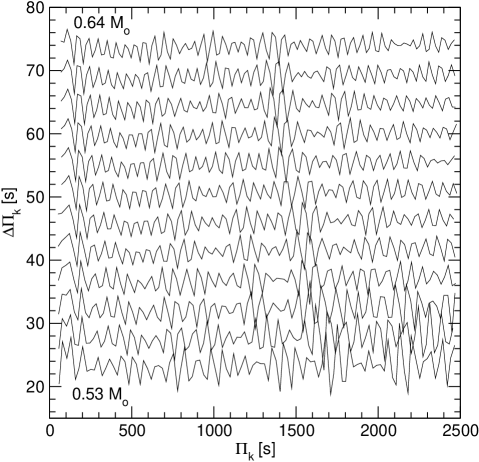
Figure 13: The period-spacing distributions for PG 1159 models with stellar masses, from bottom to top: $0.53,0.54,\ldots,0.64M_{\odot}$ at $T_{\rm eff}\approx 140\,000$ K. In the interests of clarity, each curve has been arbitrarily shifted upwards, starting from the lowest one, corresponding to the model with $M_{*}=0.53M_{\odot}$. Models with stellar masses other than $0.5895$-$M_{\odot}$correspond to evolutionary stages after the unphysical transitory phase (induced by the scaling of the stellar mass) has long vanished.

3.5 The effect of changes in the stellar mass

In the above discussion we have been able to identify the physical origins and nature of mode trapping in our PG 1159 models. We wish now to explore the effect of changing the stellar mass $M_{*}$ on the period-spacing diagrams and mode trapping. As mentioned previously, we have employed in this project model sequences with stellar masses in the ranges $0.53-0.58$ $M_{\odot}$  and $0.60-0.64$ $M_{\odot}$  with a step of 0.01 $M_{\odot}$ , in addition to the 0.5895-$M_{\odot}$  sequence previously described. We recall that those sequences were obtained from the 0.5895-$M_{\odot}$  sequence by artificially changing the stellar mass according the procedure outlined in §2. Thus, we caution that the results derived in this section could change if the complete evolution of progenitor stars with different stellar masses were accounted for. From the asymptotic theory outlined in §3.3, we know that $\Delta\Pi_{\ell}^{\rm a}$ decreases when the stellar mass increases, as it is evident from Fig. 9. As mentioned previously, the asymptotic period spacing is very close to the average of the computed period spacings $\overline{\Delta\Pi_{k}}$. As a result, the average of the computed period spacing also must decreases as the stellar mass increases. In fact, $\overline{\Delta\Pi_{k}}$ decreases from $23.19$ s to $18.69$ s when we increase the stellar mass from $0.53M_{\odot}$ to $0.64M_{\odot}$ for a fixed $T_{\rm eff}\approx 140\,000$ K.

We also expect variations in the amplitude and cycle of trapping when we consider changes in the stellar mass. In Fig. 13 we depict period-spacing diagrams for PG 1159 models with values of $M_{*}$ covering the complete set of stellar masses considered in this work, and for a fixed effective temperature of $\approx 140\,000$ K. Note that the trapping amplitude decreases when the stellar mass increases. In fact, the maximum of the trapping amplitude is of about $10$ s for $0.53M_{\odot}$, whereas it assumes a value of $\approx 5$ s, at most, for $0.64M_{\odot}$. This is a direct consequence of an increased electron degeneracy in the core of our more massive models, which in turn produces a weakening in the efficiency of mode trapping. Other striking feature observed in Fig. 13 is the decrease in the period of the trapping cycle and the shift of mode trapping features to lower periods as we go to larger values of the stellar mass. Specifically, the portions of the period-spacing diagram centered at $\approx 500,\approx 900,\approx 1400,\approx 1700$ and $\approx 2200$ s for the model with $M_{*}=0.53M_{\odot}$, move to regions centered at $\approx 100,\approx 700,\approx 1000,\approx 1400$ and $\approx 1900$ s, respectively, for the model with $M_{*}=0.64M_{\odot}$. This effect can be understood on the basis that, while the O/C chemical structure remains at the same $M_{r}/M_{*}$ value inside the model when we consider higher stellar masses, its location in terms of the radial coordinate ($r$) shifts away from the stellar centre, from $r/R\approx 0.22$ for $M_{*}=0.53M_{\odot}$ to $r/R\approx 0.33$ for $M_{*}=0.64M_{\odot}$. A similar effect has been found by Córsico et al. (2005) in the context of crystallizing ZZ Ceti models, by considering a fixed value of $M_{*}$ but with the inner turning point of the $g$-mode eigenfunctions — the crystallization front — moving outwards.

3.6 The effect of changes in the effective temperature

In closing this section, we shall explore the evolution of the mode-trapping properties as our PG 1159 evolve to cooler temperatures. As we mentioned earlier, the asymptotic period spacing $\Delta\Pi_{\ell}^{\rm a}$ and the average of the computed period spacings $\overline{\Delta\Pi_{k}}$ increase when the stellar luminosity decreases (see Fig. 9). When the star evolves along the WD cooling track, a decreasing effective temperature is usually associated to a decreasing stellar luminosity. As a result, we also expect that $\Delta\Pi_{\ell}^{\rm a}$ and $\overline{\Delta\Pi_{k}}$ increase as cooling proceeds. This trend is confirmed by our pulsation computations. In fact, $\overline{\Delta\Pi_{k}}$ increases from $20.22$ s to $\approx 24.12$ s when the effective temperature is decreased from $170\,000$ K to $70\,000$ K in a model with $0.5895M_{\odot}$. The explanation to this effect is straightforward. As the star cools their core becomes more degenerate and the Brunt-Väisälä frequency decreases because $\chi_{\rm T}$ goes down (see Eq. 1). As a result, the pulsation periods become longer and thus the period spacing and the average of the period spacing must increase.

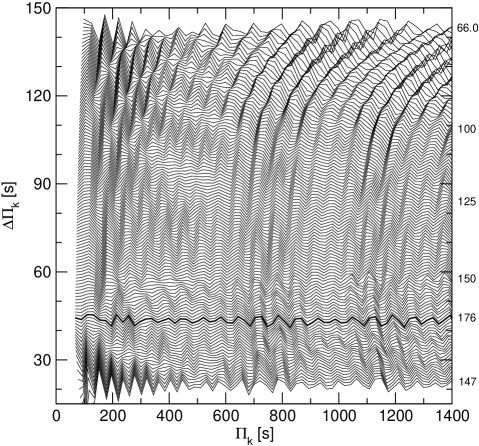
Figure 14: Period-spacing distributions for 0.5895-$M_{\odot}$  PG 1159 models at different effective temperatures. In the interests of clarity, each curve has been shifted upwards, except for the lowest one. In a few cases we have included numbers at the right side of the plot, corresponding to the $T_{\rm eff}$ value of the models (in units of kK). In particular, the thick curve corresponds to the highest value of effective temperature reached by the star, $T_{\rm eff}\sim 176$ kK.

Now, we want to see the effect of changes in the effective temperature on the trapping cycle and amplitude. To have a global picture of what happens when the effective temperature changes, we depict in Fig. 14 the evolution of the period spacing for 0.5895-$M_{\odot}$  models, shown at different effective temperatures (indicated at the right side of the plot) starting from a stage in which the model is still approaching its maximum $T_{\rm eff}$ (lowest curve) until to a phase in which the object is already on the WD cooling track (upper curve). Note that the scale at left of the plot has sense only for the lowest curve; the remaining curves are shifted upward with purposes of clarity. The figure emphasizes the notable changes that undergoes the period-spacing structure as the effective temperature varies. Note that there exist two clearly different trends. In stages in which the effective temperature increases (before the star reaches its hot turning point at $T_{\rm eff}\approx 176,000$ K) the mode-trapping features slowly move toward short periods. This is due to the fact that pulsation periods decrease in response of the overall warming of the star, and that the outer layers contract. When the star has already passed through its hottest phase, the opposite behavior is exhibited by the mode-trapping features. Indeed, maxima and minima values of the period-spacing distributions move to higher periods when the effective temperature diminishes, in particular below $T_{\rm eff}\approx 100\,000$ K. Finally, we note that the trapping amplitude increases when the effective temperature decreases.

4 Application to real stars: asteroseismology of variable GW Vir stars

In this section we shall attempt to infer the main structural parameters (that is, $M_{*}$ and $T_{\rm eff}$) of several GW Vir stars by employing the results of our extensive period computations described in previous sections. Due to the fact that in this project we have not been able to compute realistic PG 1159 models with stellar masses other than $0.5895M_{\odot}$ in the low-gravity phases (before the star reaches the “knee” at the highest value of $T_{\rm eff}$; see Fig. 1), we have limited ourselves to make seismic inferences only for the high-gravity members of the GW Vir class, that is, the naked — stars without surrounding nebulae — variables PG 1159-035, PG 2131+066, PG 1707+427, and PG 0122+200. We mention that the results described below are conditional on the assumption under the sequences of different stellar masses have been created (see Sect. 2). As it is well known, changes in the thickness of the surface helium-rich layer and in the surface composition affect the trapping cycle and amplitude (see KB94). Thus, by adopting these quantities as free adjustable parameters it is possible to perform a fine tunning of the trapping cycle and the trapping amplitude to best match the period spectrum of a given star. In spite of this, in this work we prefer to keep fixed the thickness of the helium layer and the surface composition by adopting for these parameters the values predicted by our evolutionary computations. It is worth to mention that all of these naked GW Vir stars exhibit very similar surface abundances $(X_{\rm H},X_{\rm He},X_{\rm C},X_{\rm O})\approx(0.00,0.33,0.50,0.17)$. Our PG 1159 models are characterized by surface abundances of (0.000, 0.306, 0.376, 0.228), and thus, they are very appropriate for our purposes. Before going to seismic applications of our bank of periods, we summarize the basic properties of the cited GW Vir stars below.

The four naked GW Vir stars have higher gravity ($\log g\gtrsim 7$) than the PNNVs, and they are thought to be slightly more evolved. From a pulsation point of view, the only difference between both types of variable stars is that PNNV stars in general pulsate with longer periods — in the range of about $1000-3000$ s — than the naked GW Vir — which pulsate with periods below 1000 s. Specifically, there is a well-defined correlation between the luminosity of the star and the periods exhibited: the more luminous the star is, the longer the pulsation periods are.

– PG 1159-035: this is the prototype of the PG 1159 spectral class, and also the prototype of the GW Vir pulsators. After the discovery of its variability by McGraw et al. (1979), PG 1159-035 became the target of an intense observational scrutiny. The most fruitful analysis of its light curve was carried out by Winget et al. (1991) employing the high-quality data from the Whole Earth Telescope (WET; Nather et al. 1990). This analysis showed that PG 1159-035 pulsate in more than 100 independent modes with periods between 300 and 800 s. By using 20 unambiguously identified $\ell=1,m=0$ periods between 430 and 817 s, KB94 determined a mass for PG 1159-035 of $0.59M_{\odot}$, an effective temperature of $T_{\rm eff}=136\,000$ K and a surface gravity of $\log g=7.4$. In addition, a stellar luminosity of $195L_{\odot}$ and a distance of $440$ pc from the Earth were inferred. On the other hand, spectroscopic analysis by Dreizler & Heber (1998) yield $T_{\rm eff}=140\,000$ K and $\log g=7$, in good agreement with the asteroseismic fit of KB94, but a higher luminosity of $501L_{\odot}$.

– PG 2131+066: Was discovered as a variable star by Bond et al. (1984) with periods of about 414 and 386 s, along with some other periodicities. On the basis of an augmented set of periods from WET data, Kawaler et al. (1995) considered a $T_{\rm eff}=80\,000$ K and obtained a precise mass determination of $M_{*}=0.61M_{\odot}$, a luminosity of $10L_{\odot}$ and a distance from the Earth of $470$ pc. Spectroscopic constraints of Dreizler & Heber (1998) give $M_{*}=0.55M_{\odot}$, $T_{\rm eff}=95\,000$ K, $39.8L_{\odot}$ and $\log g=7.5$ for PG 2131+066. By using the updated Dreizler & Heber (1998)’s determination of the effective temperature, Reed et al. (2000) refined the procedure of Kawaler et al. (1995). They found $M_{*}=0.608M_{\odot}$, a luminosity of $26L_{\odot}$ and a seismic distance to PG 2131+066 of $668$ pc.

– PG 1707+427: This star was discovered to be a pulsator by Bond et al. (1984). Dreizler & Heber (1998) obtained $T_{\rm eff}=85\,000$ K and $\log g=7.5$, and a stellar mass and luminosity of $0.54M_{\odot}$ and $25L_{\odot}$, respectively, were inferred from their spectroscopic study. Recently, Kawaler et al. (2004) have reported the analysis of multisite observations of PG 1707+427 obtained with WET. Preliminary model fits by using 7 independent $\ell=1$ modes with periods between 334 and 910 ssuggest an asteroseismic mass and luminosity of $0.57M_{\odot}$ and $23L_{\odot}$, respectively.

– PG 0122+200: It is the coolest GW Vir variable, with $T_{\rm eff}=80\,000$ K and $L_{*}=20L_{\odot}$ (Dreizler & Heber 1998). Spectroscopy indicates a stellar mass of $0.53M_{\odot}$ and a gravity of $\log g=7.5$. By employing an analysis based on multisite observations with WET, O’Brien et al. (1998) report a seismic stellar mass of $0.69M_{\odot}$, strikingly higher than the spectroscopic estimation. The cooling of PG 0122+200 appears to be dominated by neutrino looses; this renders PG 0122+200 as the prime target for learning neutrino physics (O’Brien et al. 1998).

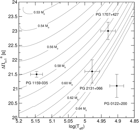
Figure 15: The asymptotic period spacing for PG 1159 models with stellar masses of $0.53,\cdots,0.64M_{\odot}$ in terms of the effective temperature. This figure is based on Fig. 9. The observed mean period spacing $\overline{\Delta\Pi}$ of the high-gravity GW Vir stars PG 1159-035, PG 2131+066, PG 1707+427, and PG 0122+200 ($21.5\pm 0.1$ s, $21.6\pm 0.4$ s, $23.0\pm 0.3$ s and $21.1\pm 0.4$ s, respectively) is also shown (taken from Kawaler et al. 2004).

Table 1: The values of the stellar mass (in $M_{\odot}$) from spectroscopic and asteroseismic studies, and the values obtained in this work from three different methods.

Source	PG 1159$-$035	PG 2131+066	PG 1707+427	PG 0122+200
Spectroscopy	$0.54\pm 0.1^{\rm(a)}$	$0.55\pm 0.1^{\rm(a)}$	$0.54\pm 0.1^{\rm(a)}$	$0.53\pm 0.1^{\rm(a)}$
Asteroseismology	$0.59\pm 0.01^{\rm(b)}$	$0.61\pm 0.02^{\rm(c)}$	$0.57\pm 0.02^{\rm(d)}$	$0.69\pm 0.04^{\rm(e)}$
By comparing $\overline{\Delta\Pi}$ with $\Delta\Pi_{\ell}^{\rm a}$ (this work)	$0.575\pm 0.005$	$0.615\pm 0.015$	$0.595\pm 0.015$	$0.70\pm 0.02$
By comparing $\overline{\Delta\Pi}$ with $\overline{\Delta\Pi_{k}}$ (this work)	$0.555\pm 0.005$	$0.575\pm 0.015$	$0.565\pm 0.015$	$0.64\pm 0.02$
By means of $\chi^{2}$ period fittings (this work)	$0.56\pm 0.01$	$0.60\pm 0.01$	$0.55\pm 0.01$	$0.64\pm 0.01$

References: (a) Dreizler & Heber (1998); (b) KB94; (c) Reed et al. (2000); (d) Kawaler et al. (2004); (e) O’Brien (2000)

In order to infer the structural parameters of these four GW Vir stars, we shall employ three different methods. First, we estimate the stellar masses by using the asymptotic period spacing of our models, as computed from Eq. (4). Specifically, we make a direct comparison between $\Delta\Pi_{\ell}^{\rm a}$ and the observed mean period spacing $\overline{\Delta\Pi}$, assuming that the effective temperature of the target star is that obtained by means of spectroscopy. In the second approach, we repeat this procedure but this time using the average of the computed period spacings $\overline{\Delta\Pi_{k}}$ and comparing it with the observed mean period spacing $\overline{\Delta\Pi}$. The third approach is a fitting method in which we compare the theoretical ($\Pi_{k}^{\rm T}$) and observed ($\Pi_{i}^{\rm O}$) periods by means of a standard $\chi^{2}$ algorithm. In the three approachs we assume that the observed periods correspond to $\ell=1,m=0$ modes.

4.1 Inferences from the asymptotic period spacing, $\Delta\Pi_{\ell}^{\rm a}$

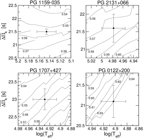
Figure 16: The average of the computed period spacings for PG 1159 models with different stellar masses in terms of the effective temperature. Each panel corresponds to a specific GW Vir star. The observed mean period spacing $\overline{\Delta\Pi}$ is also shown (taken from Kawaler et al. 2004).

We start by examining Fig. 15, in which the asymptotic period spacing ($\Delta\Pi_{\ell}^{\rm a}$) is shown in terms of the effective temperature for PG 1159 sequences with stellar masses of $0.53,\cdots,0.64M_{\odot}$. We also include in the figure the values of the observed mean period spacing, $\overline{\Delta\Pi}$, corresponding to the GW Vir stars PG 1159-035, PG 2131+066, PG 1707+427, and PG 0122+200. The values of $\overline{\Delta\Pi}$ and the associated error bars are taken from Table 6 of Kawaler et al. (2004). In Table 1 we summarize our results. Note that the spectroscopic estimation of $T_{\rm eff}$ for PG 0122+200 place it at an effective temperature that is lower than our PG 1159 models. Thus, for PG 0122+200 we can only make a rough extrapolation. Note the notable agreement between our estimates and the values inferred by other pulsation studies. Note also that the seismic inferences suggest higher mass values as compared with the spectroscopic estimations. We do not actually understand the origin of this discrepancy, but we note that spectroscopic derivations of the stellar mass are usually very uncertain due to the large uncertainty in the determination of $\log g$ — an error of $0.3$ dex translates into an error of $0.1M_{\odot}$ (Dreizler & Heber 1998). Indeed, Dreizler & Heber (1998) first estimate $\log g$ and $T_{\rm eff}$ values by using fits to model atmospheres, and then they select the stellar mass from the evolutionary tracks of O’Brien (2000). Thus, both the large uncertainties in the estimation of $\log g$ ($\approx$ 0.5 dex) and in the evolutionary computations could account for an excessively broad range of allowed masses for a specific star.

4.2 Inferences from the average of the computed period spacings, $\overline{\Delta\Pi_{k}}$

Here, we repeat the procedure described in §4.1, but this time by employing the average of the computed period spacings ($\overline{\Delta\Pi_{k}}$) instead the asymptotic period spacing. We compare $\overline{\Delta\Pi_{k}}$ with the measured $\overline{\Delta\Pi}$ for each star under consideration. In computing the average of the computed period spacings, we consider only the period interval in which the periodicities of a given star are observed. For instance, for PG 1159-035, we compute the average of the computed period spacings for periods in the range [430, 841] s. The results of our calculations are shown in Fig.16, in which we show $\overline{\Delta\Pi_{k}}$ plotted with dashed lines in terms of $T_{\rm eff}$ for the four GW Vir stars under consideration. Note that, since we have performed the average of the computed period spacings on different period ranges, appropriate to the period range exhibited by a specific star, the curves of $\overline{\Delta\Pi_{k}}$ are different in each panel. In Table 1 we include the estimations of the stellar mass for the four stars. Note that the stellar masses as determined by this approach are appreciably lower than the values inferred by using the asymptotic period spacing and thus in better agreement with spectroscopic inferences. This is due to $\overline{\Delta\Pi_{k}}$ is typically $\approx 0.8-1.0$ s smaller than $\Delta\Pi_{\ell}^{\rm a}$, irrespective of the stellar mass and effective temperature. Thus, if we compare the observed mean period spacing for a given star with $\overline{\Delta\Pi_{k}}$ we obtain a smaller total mass ($0.02-0.06M_{\odot}$ lower) than that inferred by comparing the observed mean period spacing with $\Delta\Pi_{\ell}^{\rm a}$. We stress that the asymptotic period spacing $\Delta\Pi_{\ell}^{\rm a}$, as computed by means of Eq. 4, is formally valid for the limit of high radial order $k$ in chemically homogeneous stars. Because our PG1159 models are chemically stratified, we conclude that the estimations of $M_{*}$ from $\overline{\Delta\Pi_{k}}$ are more realistic than those inferred by means of $\Delta\Pi_{\ell}^{\rm a}$. We also found that our $M_{*}$ values are lower than those quoted by other seismic studies (see Table 1). We note that, with the exception of the work of KB94 for PG 1159-035, all these studies compare the observed mean period spacing with the asymptotic predictions to infer the stellar mass. Thus, not surprisingly, their values are very similar to our results obtained from the asymptotic period spacing in §4.1, but rather departed from our values deduced from the average of the computed period spacings.

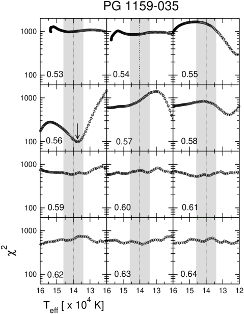
Figure 17: The $\chi^{2}$ values as defined by Eq. (5) corresponding to PG 1159-035 versus the effective temperature for $\ell=1$ modes. Each panel depicts the results for a specific mass value. The gray strip corresponds to the allowed values of $T_{\rm eff}$ according to spectroscopic measurements. The arrow indicate the minimum value of $\chi^{2}$ associated with the effective temperature of the best-fit model.

4.3 Inferences from the computed pulsation periods, $\Pi_{k}$

We turn now to the $\chi^{2}$ period fitting procedure. The goodness of a given fit is measured by means of a quality function, defined as

$$\chi^{2}(M_{*},T_{\rm eff})=\sum_{i=1}^{N}\min[(\Pi_{i}^{\rm O}-\Pi_{k}^{\rm T})^{2}].$$ (5)

Table 2: Comparison between the observed periods of PG 1159-035 (taken from KB94) and theoretical ($\ell=1$) periods of the best-fit model ($\overline{\delta\Pi}=1.79$ s, $\sigma_{\delta\Pi}=2.21$ s).

$\Pi_{i}^{\rm O}$	$\Pi_{k}^{\rm T}$	$k$	$\delta\Pi_{i}$	$\delta\Pi_{i}/\Pi_{i}$
$[$s$]$	$[$s$]$		$[$s$]$	$[\%]$
$430.04$	$433.21$	18	$-3.17$	$-0.74$
$450.71$	$453.49$	19	$-2.78$	$-0.62$
$469.57$	$473.51$	20	$-3.94$	$-0.84$
$494.85$	$496.58$	21	$-1.73$	$-0.35$
$517.18$	$517.10$	22	$0.08$	$0.02$
$538.16$	$537.50$	23	$0.66$	$0.12$
$558.44$	$559.15$	24	$-0.71$	$-0.13$
$581.29$	$580.55$	25	$0.74$	$0.13$
$603.04$	$601.28$	26	$1.76$	$0.29$
$622.60$	$622.60$	27	$0.00$	$0.00$
$643.41$	$645.24$	28	$-1.83$	$-0.28$
$666.22$	$665.09$	29	$1.13$	$0.17$
$687.71$	$686.29$	30	$1.42$	$0.21$
$707.92$	$709.95$	31	$-2.03$	$-0.29$
$729.50$	$729.65$	32	$-0.15$	$-0.02$
$753.12$	$750.01$	33	$3.11$	$0.41$
$773.77$	$773.33$	34	$0.44$	$0.06$
$790.94$	$795.17$	35	$-4.23$	$-0.53$
$817.12$	$814.96$	36	$2.16$	$0.26$
$840.02$	$836.27$	37	$3.75$	$0.45$

Here, $\Pi_{i}^{\rm O}$ is one of the $N$ observed pulsation periods, and $\Pi_{k}^{\rm T}$ is a specific computed period with radial index $k$. The method consists of looking for the PG 1159 model that shows the lowest value of $\chi^{2}$. Obviously, $\chi^{2}\rightarrow 0$ if the match between observed and computed periods were perfect. We evaluate $\chi^{2}(M_{*},T_{\rm eff})$ varying $M_{*}/M_{\odot}$ in the range $[0.53,0.64]$ with a step $\Delta(M_{*}/M_{\odot})=0.01$, whereas for the effective temperature we adopt a much more finer grid, with $\Delta T_{\rm eff}=10-20$ K.

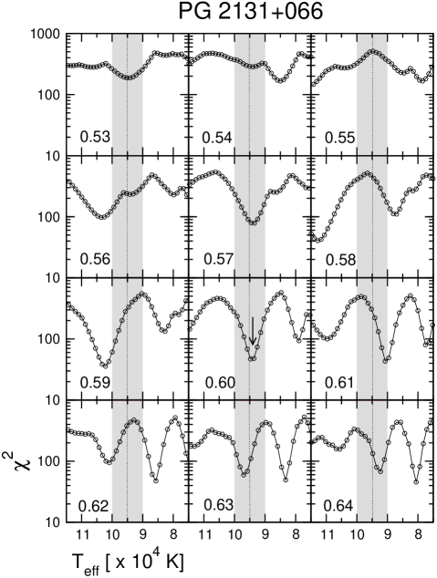
Figure 18: Same as Fig. 17, but for PG 2131+066.

We initially searched the optimal model within a wide interval of effective temperatures, ranging from the hottest point reached by the model in the H-R diagram ($160\,000-200\,000$ K, according to the value of $M_{*}$) until $T_{\rm eff}\sim 70\,000$ K. However, throughout our calculations we realized that generally the run of $\chi^{2}$ as a function of $T_{\rm eff}$ for a given star exhibits more than one minimum, meaning that the period spectrum of the star could not be fitted by an unique PG 1159 model. This behaviour is more pronounced in the case of the GW Vir stars with few observed periods available. This effect can be understood on the basis that the pulsation periods of a specific model are generally increasing with time. If at a given effective temperature the model shows a close fit to the observed periods, then the function $\chi^{2}$ reaches a local minima. When the model has cooled enough (at some time later), it is possible that the accumulated period drift nearly matches the period spacing between adjacent modes ($|\Delta k|=1$). In these circumstances, the model is able to fit the star again, as a result of which $\chi^{2}$ exhibits other local minimum. To break this degeneracy, we decided to consider a more restricted range of effective temperatures, but that still comfortably embraces the spectroscopic estimation of $T_{\rm eff}$ and its uncertainties. Specifically, in searching the “best-fit” model for a specific star we considered effective temperatures laying inside an interval $T_{\rm eff}^{\rm spec}-20,000\leq T_{\rm eff}\leq T_{\rm eff}^{\rm spec}+20\,000$ K , where $T_{\rm eff}^{\rm spec}$ is the spectroscopic determination of the effective temperature. As we shall describe below, for the star PG 1159-035 we were able to find a best-fit model for which $\chi^{2}$ adopts the lowest value within this interval of $T_{\rm eff}$s. The situation was considerably more difficult for PG 2131+066, PG 1707+427, and PG 0122+200, due to the scarcity of pulsation periods characterizing their pulsation spectra. In fact, for these stars the ambiguity associated with the existence of multiple solutions remained even when we adopted a more restricted $T_{\rm eff}$-interval, and in that cases the procedure failed to isolate the best solution. In order to solve this situation, for PG 2131+066, PG 1707+427, and PG 0122+200 we restricted the search to within $1\sigma$ of the spectroscopic value.

Table 3: Comparison between the observed periods of PG 2131+066 (taken from Kawaler et al. 1995) and the theoretical ($\ell=1$) periods of the best-fit model ($\overline{\delta\Pi}=1.83$ s, $\sigma_{\delta\Pi}=2.59$ s).

$\Pi_{i}^{\rm O}$	$\Pi_{k}^{\rm T}$	$k$	$\delta\Pi_{i}$	$\delta\Pi_{i}/\Pi_{i}$
$[$s$]$	$[$s$]$		$[$s$]$	$[\%]$
$341.45$	$341.40$	14	$0.05$	$0.014$
—	$364.21$	15	—	—
$384.27$	$382.23$	16	$2.04$	$0.53$
$403.93$	$403.86$	17	$0.07$	$0.017$
$426.36$	$425.07$	18	$1.29$	$0.30$
$450.28$	$445.17$	19	$5.11$	$1.13$
$462.39$	$466.26$	20	$-3.87$	$-0.84$
—	$486.74$	21	—	—
$507.91$	$508.27$	22	$-0.36$	$-0.07$

We start by examining Fig. 17 in which the run of $\chi^{2}$ is plotted versus $T_{\rm eff}$ for PG 1159-035. We include the results for the complete set of stellar masses considered in this work. The observed periods are the same twenty $\ell=1,m=0$ consecutive periods considered in KB94. The vertical dotted line corresponds to the effective temperature of PG 1159-035 as measured by means of spectroscopic techniques ($T_{\rm eff}^{\rm spec}=140\,000$ K). Note that there is a well-defined minima of $\chi^{2}$, indicated with an arrow in the plot, corresponding to a stellar model with $M_{*}=0.56M_{\odot}$ and $T_{\rm eff}\sim 137,000$ K. We adopt this model as our best-fit model. A comparison between the observed periods of PG 1159-035 and the theoretical periods corresponding to the best-fit model is included in Table 2. The first column lists the observed periods, and the second and third columns correspond to the computed periods and the associated radial order, respectively. The last two columns show the difference and the relative difference (in percent) between the observed and computed periods, respectively, defined as $\delta\Pi_{i}=\Pi_{i}^{\rm O}-\Pi_{k}^{\rm T}$ and $\delta\Pi_{i}/\Pi_{i}=100\times(\Pi_{i}^{\rm O}-\Pi_{k}^{\rm T})/\Pi_{i}^{\rm O}$. Note that the period match is excellent. To quantitatively measure the quality of the fit we compute the mean of the period differences, $\overline{\delta\Pi}$ and the root-mean-square residual, $\sigma_{\delta\Pi}$. We obtain $\overline{\delta\Pi}=1.79$ s and $\sigma_{\delta\Pi}=2.21$ s for the fit to PG 1159-035. The quality of our fit is comparable to that achieved by KB94 ($\overline{\delta\Pi}\sim 1.19$ s), although the KB94 fit is notoriously better. In this connection, it is interesting to note that these authors adopt $M_{\rm He}$ and the surface composition as free adjustable parameters for the period fit, in addition to the stellar mass and the effective temperature. Therefore, they are able to make a finner tuning of the observed period spectrum than our own. The structural parameters of our best-fit model are listed in Table 6. Note the rather nice agreement between our predictions and the structural properties of PG 1159-035 as inferred by other standard techniques. For instance, the effective temperature, the luminosity and the surface gravity of our best-fit model are consistent at the $1\sigma$ level with the spectroscopic estimations of Dreizler & Heber (1998). In particular, the quality function of our period fit naturally adopts an unique minimum value at an effective temperature very close to the spectroscopic value (this is not the case for the remainder GW Vir stars; see below). Note also that the total mass of our model lies at $0.02M_{\odot}$ above the spectroscopic mass, although well within the allowed range ($0.44\leq M_{*}/M_{\odot}\leq 0.64$). We stress again that spectroscopy determines only $\log g$ and $T_{\rm eff}$, and then the value of the stellar mass is assessed using evolutionary tracks, which depend on the complete evolution of the progenitors. We note that our seismological mass is lower than the value obtained by KB94 by employing the same set of observed pulsation periods.

Table 4: Comparison between the observed periods of PG 1707+427 (taken from Kawaler et al. 2004) and the theoretical ($\ell=1$) periods of the best-fit model ($\overline{\delta\Pi}=2.31$ s, $\sigma_{\delta\Pi}=2.70$ s).

$\Pi_{i}^{\rm O}$	$\Pi_{k}^{\rm T}$	$k$	$\delta\Pi_{i}$	$\delta\Pi_{i}/\Pi_{i}$
$[$s$]$	$[$s$]$		$[$s$]$	$[\%]$
$334.62$	$332.14$	12	$2.48$	$0.74$
—	$352.76$	13	—	—
—	$377.17$	14	—	—
—	$399.73$	15	—	—
—	$420.53$	16	—	—
$448.07$	$445.72$	17	$2.35$	$0.52$
—	$467.50$	18	—	—
$494.39$	$489.62$	19	$4.77$	$0.96$
—	$514.23$	20	—	—
$536.41$	$535.84$	21	$0.57$	$0.11$
—	$559.94$	22	—	—
—	$581.88$	23	—	—
—	$606.38$	24	—	—
—	$628.83$	25	—	—
—	$651.41$	26	—	—
$677.89$	$677.48$	27	$0.41$	$0.06$
—	$697.36$	28	—	—
$726.02$	$723.05$	29	$2.97$	$0.41$
$745.78$	$747.18$	30	$-1.4$	$-0.19$
—	$769.01$	31	—	—
—	$792.73$	32	—	—
—	$818.54$	33	—	—
—	$841.27$	34	—	—
—	$862.57$	35	—	—
—	$890.30$	36	—	—
$909.05$	$912.62$	37	$-3.57$	$-0.39$

Table 5: Comparison between the observed periods of PG 0122+200 (taken from Vauclair et al. 2001) and the theoretical ($\ell=1$) periods of the best-fit model ($\overline{\delta\Pi}=2.61$ s, $\sigma_{\delta\Pi}=3.55$ s).

$\Pi_{i}^{\rm O}$	$\Pi_{k}^{\rm T}$	$k$	$\delta\Pi_{i}$	$\delta\Pi_{i}/\Pi_{i}$
$[$s$]$	$[$s$]$		$[$s$]$	$[\%]$
$336.67$	$340.30$	14	$-3.63$	$-1.08$
—	$360.88$	15	—	—
$379.60$	$381.16$	16	$-1.56$	$-0.41$
$401.00$	$401.75$	17	$-0.75$	$-0.19$
—	$424.05$	18	—	—
$449.43$	$442.62$	19	$6.81$	$1.51$
$468.69$	$463.65$	20	$5.04$	$1.08$
—	$485.45$	21	—	—
—	$506.63$	22	—	—
—	$527.22$	23	—	—
—	$546.99$	24	—	—
$570.00$	$570.35$	25	$-0.35$	$-0.06$
—	$591.06$	26	—	—
$611.05$	$611.24$	27	$-0.19$	$-0.03$

At variance with PG 1159-035, the stars PG 2131+066, PG 1707+427 and PG 0122+200 exhibit very few pulsation periods in their light curves. As we already anticipated, this unfortunate fact renders any asteroseismic inference on these stars considerably more difficult. This is the reason for which most of asteroseismic studies carried so far rely on the measured period spacing only. In spite of this fact, we have attempted to apply the $\chi^{2}$ fitting method to these stars by adopting a more strict criteria, i.e., by considering as valid only solutions that guaranteed consistency at $1\sigma$ level with the spectroscopic determination of $T_{\rm eff}$. Fig. 18 shows the results for PG 2131+066. For this star the observational data consists of only the seven pulsation periods reported by Kawaler et al. (1995). Note that, at variance with the case of PG 1159-035, the function $\chi^{2}$ shows various minima compatible with $T_{\rm eff}^{\rm spec}$ in the range of effective temperatures considered. For instance, for $M_{*}=0.60M_{\odot}$ there is a remarkable minima in the immediate vicinity of the spectroscopic estimation, at $T_{\rm eff}\approx 95\,000$ K. Other comparable minimum of $\chi^{2}$ are seen also for stellar masses of $0.61,0.63$ and $0.64M_{\odot}$, but at effective temperatures somewhat departed from the spectroscopic value. These minima represent equivalent solutions from the point of view of the magnitude of $\chi^{2}$, and thus, there are various possible optimal models. We elect to adopt as the best-fit model to that having the effective temperature closer to the spectroscopic determination, that is, the model with $M_{*}=0.60M_{\odot}$ and $T_{\rm eff}=94\,740$ K (indicated with an arrow in Fig. 18). A comparison between the observed periods of PG 2131+066 and the theoretical ($\ell=1$) periods of the best-fit model is given in Table 3. We note that the overall quality of the fit ($\overline{\delta\Pi}=1.83$ s, $\sigma_{\delta\Pi}=2.59$ s) is nearly so satisfactory as in the case of PG 1159-035 (Table 2). The characteristics of our best-fit model for PG 2131+066 are listed in Table 6. Our results are in good agreement with spectroscopy, although our determination of the stellar mass is significantly higher — but even consistent at the $1\sigma$ level. Note that the disagreement in the estimation of the stellar mass would be more pronounced if we were adopting anyone of the other acceptable solutions, for which $M_{*}\gtrsim 0.60M_{\odot}$.

Table 6: Summary of the seismic inferences for PG 1159-035, PG 2131+066, PG 1707+427 and PG 0122+200 from $\chi^{2}$ period fits. In the interest of comparison, we include values of structural properties extracted from spectroscopic determinations and the values of the observed mean period spacing extracted from Table 6 of Kawaler et al. (2004).

Quantity	Model	PG 1159-035	Model	PG 2131+066	Model	PG 1707+427	Model	PG 0122+200
$\overline{\Delta\Pi}$ [s]	21.21	$21.5\pm 0.1$	$20.86$	$21.6\pm 0.4$	23.22	$23.0\pm 0.3$	20.92	$21.10\pm 0.4$
$T_{\rm eff}$ [K]	137 620	$140\,000\pm 6\,000$	94 740	$95\,000\pm 5\,000$	87 585	$85\,000\pm 4\,500$	81 810	$80\,000\pm 4\,000$
$M_{*}/M_{\odot}$	0.56	$0.54\pm 0.1$	0.60	$0.55\pm 0.1$	0.55	$0.54\pm 0.1$	0.64	$0.54\pm 0.1$
$\log g$ [cm/s2]	7.31	$7.0\pm 0.3$	7.71	$7.5\pm 0.3$	7.59	$7.5\pm 0.3$	7.89	$7.5\pm 0.3$
$\log(L_{*}/L_{\odot})$	2.38	$2.7\pm 0.4$	1.37	$1.6\pm 0.3$	1.31	$1.4\pm 0.3$	0.96	$1.3\pm 0.3$
$R_{*}/R_{\odot}$	0.0273	—	0.0179	—	0.02	—	0.015	—
$M_{\rm He}$ $[10^{-3}M_{\odot}]$	$4.94$	—	$5.29$	—	$4.85$	—	$5.65$	—
distance [pc]	$482\pm 44$	$800^{+600{\rm(a)}}_{-400}$	$716^{+185}_{-147}$	$681^{+170{\rm(b)}}_{-137}$	$697^{+180}_{-144}$	$1300^{+1000{\rm(a)}}_{-600}$

References: (a) Werner et al. (1991); (b) Reed et al. (2000)

We have also applied our fitting procedure to the GW Vir stars PG 1707+427 and PG 0122+200. We have found that the behavior of $\chi^{2}$ in these cases is, not surprisingly, very similar to that shown by Fig. 18 for PG 02131+066, because these stars also exhibit a very reduced number of pulsation periods. Therefore, to obtain optimal representative models we employ the same procedure than in the case of PG 02131+066, i.e., we consider as valid the solutions that are consistent at $1\sigma$ with the spectroscopically inferred effective temperature. In this way we discard other possible solutions at effective temperatures that do not match the spectroscopic evidence. The results are summarized in Tables 4 and 5, respectively. Note that for PG 1707+427 the period match is of a slightly lower quality than for PG 1159-035 and PG 2131+066, but still satisfactory, with $\overline{\delta\Pi}=2.31$ s and $\sigma_{\delta\Pi}=2.70$ s. For PG 0122+200, however, the fit is considerably worse, being $\overline{\delta\Pi}=2.61$ s and $\sigma_{\delta\Pi}=3.55$ s. The main source of discrepancy comes from the existence of periods at 449.43 and 468.69 s. We mention that for PG 0122+200 we have also considered the set of observed periods reported by O’Brien et al. (1998), which do not includes the period at 468.69 s. We find that the quality of the fit in that case do not improves significantly. The structural properties of the best-fit models for PG 1707+427 and PG 0122+200 are given in Table 6. For PG 1707+427 we found a general agreement between our inferences and the spectroscopic values, in particular concerning the stellar mass. In the case of PG 0122+200 we found a total mass and a surface gravity large in excess as compared with the spectroscopic evidence. This high mass value is in line with other seismic determinations and also with our own predictions based on the asymptotic period spacing and the average of the computed period spacings (see Table1).

In addition to the structural properties of the GW Vir stars under study, we infer their “seismic” distance from the Earth. First, we compute the bolometric magnitude from the luminosity of the best-fit model, by means of $M_{\rm bol}=M_{\odot{\rm bol}}-2.5\log(L_{*}/L_{\odot})$, with $M_{\odot{\rm bol}}=4.75$ (Allen 1973). Next, we transform the bolometric magnitude into the absolute magnitude, $M_{\rm v}=M_{\rm bol}-{\rm BC}$, where ${\rm BC}$ is the bolometric correction. Finally, we compute the seismic distance according to $\log d\ [{\rm pc}]=\frac{1}{5}\left(m_{\rm v}-M_{\rm v}+5\right)$. For PG 1159-035 ($m_{\rm v}=14.84$) we adopt a bolometric correction of ${\rm BC}=-7.6\pm 0.2$ from KB94. Following Kawaler et al. (1995), we adopt ${\rm BC}=-6.0\pm 0.5$ for PG 2131+066 ($m_{\rm v}=16.6$) and PG 1707+427 ($m_{\rm v}=16.69$). Unfortunately, there is not available any estimation of the bolometric correction for PG 0112+200, hindering any attempt to infer its seismic distance. Our seismic distances are shown in Table 6. In addition, we include the distances estimated by means of other techniques. We found a good agreement (within $1\sigma$) between our distances and the other non-seismic estimations, although our values are characterized by errors much smaller. Our results are also consistent with the distances obtained seismologically by KB94 for PG 1159-035 ($d=440\pm 40$ pc) and by Reed et al. (2000) for PG 2131+066 ($d=668^{+78}_{-83}$ pc).

5 Conclusions

In this paper we have studied in detail some relevant aspects of the adiabatic pulsations of GW Vir stars by using state-of-the-art evolutionary PG 1159 models recently presented by Althaus et al. (2005). As far as we are aware, this is the first time that the adiabatic pulsation properties of fully evolutionary post born-again PG 1159 models like the ones employed in this work are assessed. We refer the interested reader to the paper by Gautschy et al. (2005) for details about the non-adiabatic pulsation properties of these models.

We first explored the basic nature of the pulsation modes by employing propagation diagrams and weight functions. In line with previous works, our results suggest that for PG 1159 models at high luminosity stages, the propagation diagrams are reminiscent of those of their progenitors — red giant stars — characterized by large values of the Brunt-Väisälä frequency in the central regions of the star. As a result, pulsation $g$-modes — the only observed so far in GW Vir stars — are strongly confined to the highly condensed core, whereas $p$-modes are free to oscillate in more external regions. In addition, we have found that there exist several modes exhibiting a mixed nature, behaving as $p$-modes in outer regions and like $g$-modes in the deeper zones within the star. As the effective temperature increases these modes undergoes several episodes of avoided crossing. We found that pulsation periods generally decrease with time, an effect attributable to the rapid contraction experienced by the star in their incursion to the blue in the H-R diagram. Note that a decreasing period implies negative temporal rate of period change; according to our results, this is the case for all the modes during the contraction stage. Once the models have passed their maximum effective temperature and have settled onto the WD cooling track, the Brunt-Väisälä frequency acquires a more familiar shape, typical of the WD pulsators. In this phase all the pulsation periods increase with decreasing effective temperature, reflecting a lowering in the magnitude of the Brunt-Väisälä frequency at the core regions. At this stages, $g$-modes become envelope modes, and, as indicated by the weight functions, the outer regions of the star are the more relevant ones in establishing the periods. By the contrary, pulsation $p$-modes are almost confined to the degenerate core. We note that, since all the periods increase during this phase, the rate of period change for any pulsation mode must be positive. In particular, the measured rate of period change of the period at $\sim 516$ s in PG 1159-035 is positive (Costa et al. 1999), in agreement with our findings. We defer to a future work a complete discussion of the rate of period change of our PG 1159 models.

We next have focused our attention on the evolutionary stages in which the star has already entered its WD cooling track. For these phases we have been able to obtain additional evolutionary sequences with several values of the stellar mass, allowing us to study the effects of $M_{*}$ and the effective temperature on the pulsation properties of our models. In particular, we have examined the asymptotic behavior of the $g$-mode pulsations. In agreement with previous works, we found that the asymptotic period spacing increases with a decrease in the stellar mass and with an increment in the luminosity, although the dependence on the stellar mass is stronger. This fact renders the value of the period spacing observed in a given star a powerful indicator of the total mass.

The study of the mode-trapping properties of our models has been other relevant aim of the present work. In this connection, we have demonstrated that the mode-trapping features characterizing our PG1159 models are produced mostly by the shape of the O/C chemical profile at the core, at least for the range of periods observed in GW Vir stars. On their hand, the outer chemical interface of O/C/He produces negligible mode-trapping effects, except for the regime of short periods in the pulsation spectrum. This conclusion is at odds with previous results reported by KB94, who realized that the mode-trapping properties of their PG 1159 models were fixed essentially by the outer O/C/He transition region. We have found that the origin of this discrepancy rests on the differences in the input physics employed in build up the background stellar models. Specifically, the main difference is the presence of a much less pronounced chemical transition in the outer parts of the C/O core of the KB94 models, as compared with the rather abrupt chemical gradients at $M_{r}\approx 0.4-0.6M_{*}$ in our PG 1159 models. Other ingredient that contributes to the disagreement between our results and those of KB94 is the thickness of the helium envelope. Indeed, since our models are characterized by thick helium envelopes ($M_{\rm He}\sim 0.0052M_{\odot}$), the mode trapping effects caused by the O/C/He transition region are much more weaker than in the models of KB94.

We note that the structure of the core chemical profile of our PG 1159 models is the relic of convective overshoot episodes during the central helium burning phase. The sensitivity of the mode trapping effects to the details of the core chemical structure rises the possibility of employing pulsating PG 1159 and WD stars to constrain the efficiency of extra mixing episodes in the core of their progenitors (overshooting and/or semiconvection; see Straniero et al. 2003). This appealing issue has been recently explored by Córsico & Althaus (2005).

To gain additional insight into the nature of mode trapping in our models, we have examined the kinetic energy and weight functions of individual pulsation modes. We have found that modes showing primary maxima in the kinetic energy distribution are associated with minima in the period-spacing diagrams. By consulting the eigenfunctions and weight functions of these modes we found that they have relatively high amplitude at the high-density environment of the stellar core, and very low amplitudes in the rest of the star. The existence of these “core-trapped” modes is encountered also in the context of ZZ Ceti pulsations, as reported by Althaus et al. (2003) and Córsico et al. (2005).

Finally, we have made some preliminar seismic inferences about the internal structure and basic parameters of the GW Vir stars PG 1159-035, PG 2131+066, PG 1707+427, and PG 0122+200. To this end we have adopted three different approaches. First, we estimate the stellar masses by comparing the asymptotic period spacing with the observed mean period spacing, assuming that the effective temperature of the target star is that predicted by spectroscopy. In the second method, we repeated the above procedure but this time using the average of the computed period spacings and comparing it with the observed mean period spacing. The third approach is a fitting method in which we search for an optimal stellar model that best reproduces the observed periods. To this end we employ a quality function that measures the distance between the observed and the computed adiabatic pulsation periods within a grid of models with different effective temperatures and stellar masses.

The stellar masses we obtained from these methods are given in Table 1. Note that, except for PG 0122+200, our values are consistent with the spectroscopic inferences, particularly when the average of the computed period spacings are used, although our masses are slightly larger. For PG 0122+200 we obtain, in agreement with the seismic determination of O’Brien (2000), a large value of the stellar mass. Thus, according the pulsation theory this star seems to be the most massive among the high-gravity GW Vir pulsators. Note also that the stellar masses as determined by employing the average of the computed period spacings are appreciably lower than the values inferred by using the asymptotic period spacing. We also found that our $M_{*}$ values are smaller than that reported by other pulsation studies. In this connection, we note that, with the exception of the work of KB94 for PG 1159-035, all these works compare the observed mean period spacing with the asymptotic predictions to infer the stellar mass. Thus, not surprisingly, their values are very close to our results obtained from the asymptotic period spacing, but somewhat different from our values deduced by employing the average of the computed period spacings.

The results from our period-fitting procedure are shown in Table 6. Taking full advantage of the numerous pulsation periods observed in PG 1159-035, we have unambiguously obtained a best-fit model with an effective temperature very close to that predicted by spectroscopy. Our asteroseismic mass of $0.56M_{\odot}$ is consistent with the spectroscopic calibration ($M_{*}=0.54M_{\odot}$) and with the preferred value of Gautschy et al. (2005) ($M_{*}=0.55M_{\odot}$), but considerably lower than the value quoted by KB94 ($M_{*}=0.59M_{\odot}$). For the remainder stars, for which we have very few observed periods available, we have also obtained representative models by employing our period-fitting procedure, but, at variance with the case of PG 1159-035, for these stars we have been forced to consider as acceptable solutions only models with an effective temperature laying within $1\sigma$ of the spectroscopic value. This stringent criteria was necessary in view of the numerous and almost equivalent minima exhibited by the quality function for these stars. Note that the period matching are considerably poorer (Tables 3, 4 and 5) as compared with the case of PG 1159-035 (Table 2). We also have estimated the “seismic” distances to the stars by employing the luminosity of the best-fit models. Our estimations (see Table 6) are consistent with other determinations.

Before closing the paper we stress that, in our view, the pulsational analysis presented here constitutes a substantial improvement as compared with previous studies. However, we believe that PG1159 evolutionary models with different stellar masses based on a complete description of the physical processes occurred in all the evolutionary stages of progenitor stars would be needed to reinforce some of our results. The development of such models is certainly critical for the assessment of the internal chemical composition characterizing GW Vir stars, an issue that is key as far as precision asteroseismology is concerned.

Finally, the evolutionary tracks employed in this investigation, as well as tabulations of $\Pi_{0}$ in terms of $L_{*}$ and $T_{\rm eff}$ for the complete set of stellar masses are freely available at our URL: http://www.fcaglp.unlp.edu.ar/evolgroup/

Appendix A Pulsation equations and adiabatic quantities

Our numerical pulsation code solves the fourth-order set of equations governing linear, nonradial, adiabatic stellar pulsations in the formulation given in Unno et al. (1989):

$$x\frac{dy_{1}}{dr}=\left(V_{g}-3\right)\ y_{1}+\left[\frac{\ell(\ell+1)}{C_{1}\omega^{2}}-V_{g}\right]\ y_{2}+V_{g}\ y_{3},$$ (6)

$$x\frac{dy_{2}}{dr}=\left(C_{1}\omega^{2}-A^{*}\right)\ y_{1}+\left(A^{*}-U+1\right)\ y_{2}-A^{*}\ y_{3},$$ (7)

$$x\frac{dy_{3}}{dr}=\left(1-U\right)\ y_{3}+\ y_{4},$$ (8)

$$x\frac{dy_{4}}{dr}=UA^{*}\ y_{1}+UV_{g}\ y_{2}+\left[\ell(\ell+1)-UV_{g}\right]\ y_{3}-U\ y_{4}.$$ (9)

The boundary conditions are, at the stellar centre ($x=0$):

$$y_{1}\ C_{1}\ \omega^{2}-\ell\ y_{2}=0,\\ \ell\ y_{3}-y_{4}=0,$$ (10)

and at the stellar surface ($x=1$):

$$y_{1}-y_{2}+y_{3}=0,\\ (\ell+1)\ y_{3}+y_{4}=0,$$ (11)

being the normalization $y_{1}=1$ at $x=1$ ($x=r/R_{*}$). The dimensionless Dziembowski’s variables (eigenvalue and eigenfunctions) are defined as

$$\omega_{k}^{2}=\frac{R_{*}^{3}}{GM_{*}}\sigma_{k}^{2},$$ (12)

and

$$y_{1}=\frac{\xi_{r}}{r},\\ \ y_{2}=\frac{1}{gr}\left(\frac{p^{\prime}}{\rho}+\Phi^{\prime}\right),$$ (13)

$$y_{3}=\frac{1}{gr}\Phi^{\prime},\\ \ y_{4}=\frac{1}{g}\frac{d\Phi^{\prime}}{dr}.$$ (14)

Here, $\xi_{r}$ is the radial Lagrangian displacement, and $p^{\prime}$, $\Phi^{\prime}$ are the Eulerian perturbation of the pressure and the gravitational potential, respectively. Pertinent dimensionless coefficients of the pulsation equations are:

$$V_{g}=\frac{gr}{c^{2}},\\ \ U=\frac{4\pi\rho r^{3}}{M_{r}},$$ (15)

$$C_{1}=\left(\frac{r}{R}\right)^{3}\left(\frac{M_{*}}{M_{r}}\right),\\ \ A^{*}=\frac{r}{g}N^{2},$$ (16)

where $c$ is the adiabatic local sound speed and $N$ the Brunt-Väisälä frequency. The remainder symbols are self-explanatory. Once the eigenvalue and eigenfunctions are computed, the code proceeds to evaluate a number of important pulsation quantities, such as the pulsation period, $\Pi_{k}$,

$$\Pi_{k}=2\pi/\sigma_{k},$$ (17)

the oscillation kinetic energy, $K_{k}$,

$$K_{k}=\frac{1}{2}(GM_{*}R_{*}^{2})\omega_{k}^{2}$$ (18)

$$\times\int_{0}^{1}x^{2}\rho\left[x^{2}y_{1}^{2}+x^{2}\frac{\ell(\ell+1)}{(C_{1}\omega_{k}^{2})^{2}}y_{2}^{2}\right]dx,$$

the weight function, $W_{k}$,

$$W_{k}(x)=(4\pi GR_{*}^{2})\frac{x^{2}\rho^{2}}{U}$$ (19)

$$\times\left[A^{*}y_{1}^{2}+V_{g}\left(y_{2}-y_{3}\right)^{2}-\frac{1}{U}\{\ell\left(\ell+1\right)y_{3}+y_{4}\}^{2}\right],$$

the variational period, $\Pi_{k}^{v}$,

$$\Pi_{k}^{v}=\sqrt{\frac{8\pi^{2}}{GM_{*}}}\ \frac{K_{k}^{1/2}}{\omega_{k}}\left[\int_{0}^{1}W_{k}(x)\ x^{2}dx\right]^{-1/2},$$ (20)

and finally, the first-order rotation splitting coefficients, $C_{k}$,

$$C_{k}=\frac{(GM_{*}R_{*}^{2})}{2K_{k}}\int_{0}^{1}\frac{x^{2}\rho}{C_{1}}\left[2x^{2}y_{1}y_{2}+\frac{x^{2}}{C_{1}\omega_{k}^{2}}y_{2}^{2}\right]dx,$$ (21)

The rotation splitting of the eigenfrequencies (assuming slow, rigid rotation) can be assesed by means of

$$\sigma_{k,m}=\sigma_{k}+m(1-C_{k})\Omega$$ (22)

where $\Omega$ is the angular speed of rotation and $m$ the azimutal quantum number.