Relative spectral lag: an new redshift indicator to measure the cosmos with gamma-ray bursts

Abstract

Using 64 ms count data for long gamma-ray bursts ( $T_{90}>$ 2.6 s), we analyze the quantity, relative spectral lag (RSL), which is defined as $\tau_{31}/FWHM_{(1)}$, where $\tau_{31}$ is the spectral lag between energy bands 1 and 3, and $FWHM_{(1)}$ denotes full width at half maximum of the pulse in energy channel 1. To get insights into features of the RSLs, we investigate in detail all the correlations between them and other parameters with a sub-sample including nine long bursts. The general cross-correlation technique is adopted to measure the lags between two different energy bands. We can derive the below conclusions. Firstly, the distribution of RSLs is normal and concentrates on around the value of 0.1. Secondly, the RSLs are weakly correlated with $FWHM$, asymmetry, peak flux ($F_{p}$), peak energy ($E_{p}$) and spectral indexes ($\alpha$ and $\beta$), while they are uncorrelated with $\tau_{31}$, hardness-ratio ($HR_{31}$) and peak time ($t_{m}$). The final but important discovery is that redshift ($z$) and peak luminosity ($L_{p}$) are strongly correlated with the RSLs which can be measured easily and directly. We find that the RSL is a good redshift and peak luminosity estimator.

1 Introduction

The temporal profiles of gamma-ray bursts (GRBs) generally exhibit very complex and variable characteristics due to overlapping between adjacent pulses (Norris et al. 1996; Quilligan et al. 2002). So far many investigations on the analysis of their light-curves especially the pulses have been made. For example, the properties of pulses such as widths, amplitudes, area of pulses and time intervals between them together with number of pulses per burst had been studied by several authors (e.g. McBreen et al. 1994, 2001, 2003; Li et al. 1996; Hurley et al. 1998; Nakar & Piran 2002; Qin et al. 2005).

In addition, some investigations associated with spectra have also been made (e.g. Kouveliotou et al. 1993; Hurley et al. 1992; Ghirlanda et al. 2004a). In particular, the spectral lag between variation signals in different energy bands not only reflects the features of spectrum evolution but also exhibits the properties of light-curve. Many researches regarding this variable had been done from many distinct aspects (see, e.g. Norris et al. 2000, 2001, 2005; Gupta et al. 2002; Kocevski & Liang 2003; Daigne & Mochkovitch 2003; Schaefer 2004; Li et al. 2004; Chen et al. 2005). It is interestingly found that unlike short GRBs the spectral lags of most long GRBs are larger than zero and concentrate on the short end of the lag distribution, near 100 ms ( Band 1997; Norris et al., 2001).

Concerning the redshift (or luminosity) indictors with GRBs, previous investigations have offered us some significant paradigms in the case of light-curves, for instance, the relations of luminosity-lag (Norris et al. 2000) and luminosity-variability (Reichart et al. 2001). A particular relation between the lag and the variability had been strongly confirmed to prove both above luminosity indicators are reliable (Schaefer et al. 2001). On the other hand, other indicators based on GRB spectral features are also constructed subsequently. They originate from either the $E_{p}-E_{iso}$ relation (Amati et al. 2002; Atteia 2003), the $E_{p}-L_{p}$ relation (e.g. Yonetoku et al. 2004) or the $E_{p}-E_{\gamma}$ relation (Ghirlanda et al. 2004b). The spectra and the light-curves are related to each other, via the spectral lag.

Norris et al. (2004, 2005) found that wide pulse width is strongly correlated with spectral lag and these two parameters may be viewed as mutual surrogates in formulations for estimating GRB luminosity and total energy. Motivated by the above-mentioned developments, our first aim is to analyze the RSLs of long bursts in order to see what the distribution of them should be. Further purpose of this work is to search for the possible relations between some other parameters and them, and then interpret them in terms of physics. Data preparation is performed in $\S$ 2. In $\S$ 3, we are going to measure some typical physical variables. $\S$ 4 shows all the results. We are about to apply the RSLs to observed data and try to reveal their physical explanations in $\S$ 5. We shall end with discussion and conclusion in $\S$ 6.

2 Data analysis of pulses

2.1 Sample selection

We use 64 ms count data selected from the current BATSE catalog for long bursts, called sample 1 including 36 sources. Note that we here only take into account these bursts with single pulse in the course of selection. The highly variable temporal structure observed in most bursts is deemed to be produced by internal shocked outflow, provided that the source emitting the relativistic flow is variable enough (e.g. Dermer & Mitman 1999; Katz 1994; Rees & Mészáros 1994; Piran, Shemi & Narayan 1993). In this case, the temporal structure generally reflects the activity of the “inner engine” that drives the bursts (Sari & Piran 1997). As a result of overlap, it is generally difficult to determine how many pulses a complex bursts should comprise or to model the shape of these pulses (Norris et al. 1996; Lee at al. 2000). Fortunately, the observed peaks have almost one-to-one correlation with the activity of the emitting source, that is to say, each pulse is permissively assumed to be associated with a separate emission episode of one burst (Kobayashi et al. 1997; Kocevski et al. 2003). On the other hand, spectra parameters for distinct pulses within a burst are different from each other, which allows us to believe the spectral lags between these pulses will behave large difference (Hakkila & Giblin 2004; Ryde et al. 2005). Therefore we let our sample be composed of the relatively simple and bright bursts dominated by a single pulse event here rather than those dim or multi-peak ones for which we could accurately calculate the spectral lags.

The method of selection is not automated program (e.g. Scargle 1998; Norris et al. 2001; Quilligan et al. 2002) but directly experienced eyes, which in a certain degree could reduce any biases either from denoising techniques or from pulse identification algorithm itself (Ryde et al. 2003). Lee et al. (2000) has found the numbers of the pulses within a burst are usually different between energy bands. In principal, a bright-independent analysis is required as the burst duration measurement needs (Bonnell et al. 1997), whereas the level of S/N should be reasonable and reliable. Based on these considerations, the criterions for our sample selection are now taken as follows: $T_{90}$ duration $>$ 2.6 s; BATSE peak flux (50-300 kev) $>$ 1.5 photons $cm^{-2}s^{-1}$; and peak count rate ($>$ 25 kev) $>$ 14000 counts $s^{-1}$. Next, we are going to process the data via background subtraction and denoising.

2.2 Background subtraction and denoising

In general, the first step in data preparation is to select the appropriate background for substraction. To handle these data as a whole, an alternative mode of processing involving background subtraction along with denoising is presented here. For each source, we take the signal data cover its full range of the pulse as possible in order to ensure the contributions of all signals to lags are considered sufficiently. From the point of view of experience, data beyond this range are regarded as the fit of the background. However, for convenience, we here prefer disposing of the whole data involving pre- and post-pulse to processing separately.

Considering the duration and background level of long bursts, we first smooth them with the DB3 wavelet with the MATLAB software and then fit them with a pulse function plus a quadratic form, namely

$$F(t)={F_{m}}(\frac{t}{t_{m}})^{r}[\frac{d}{d+r}+\frac{r}{d+r}(\frac{t}{t_{m}})^{(r+1)}]^{-\frac{r+d}{r+1}}+at^{2}+bt+c$$ (1)

where the first expression on the right is a quite flexible function (see eq. (22), Kocevski et al. 2003) applied to describe pulse shapes and the hinder quadratic term represents a background that spans the whole data. The parameter $t_{m}$ is the time of the maximum flux, $F_{m}$, of the pulse and the quantities of $r$ and $d$ are next two indexes describing the rise and decay of pulse profiles respectively. Once the part of background is subtracted from the fitted data, the remainders are pure sinal data that isn’t contaminated by background and noise in a certain error level. These signal data are just what we need to use for the analysis of spectra and light-curves.

We divide our analyses into two portions in order to achieve different goals of calculations for sample 1. One portion is to pretreat the light-curve data in energy channels 1 and 3 (i.e., 25-55 kev and 110-320 kev). Here, we define these signal data belonging to the two channels as sample 2. Another is to combine the data from all four energy channels in order to study the characteristics of the “bolometric” light-curve profile, e.g. $FWHM$ and asymmetry. To avoid confusion of the definitions, the summed signal data are called sample 3.

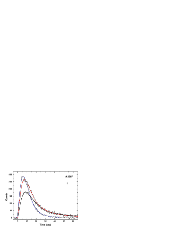
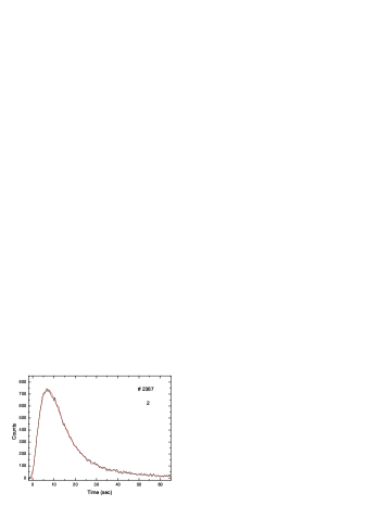
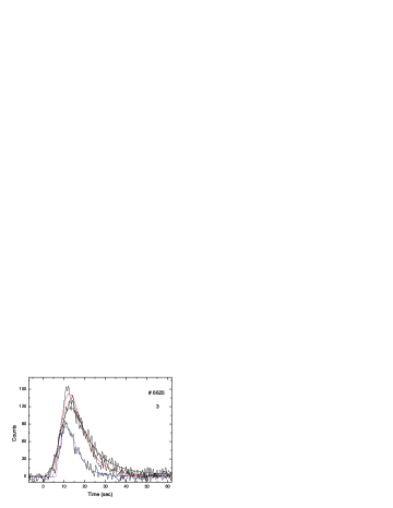
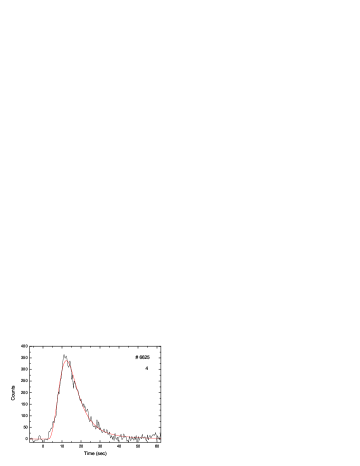
Figure 1: Light-curves of two of studied single-peaked events, GRB 930612 (# 2387, panels 1 and 2) with good S/N and GRB 980302 (# 6625, panels 3 and 4) with poor S/N. The best fit lines to observed light-curves in energy channels 1 (25-55 Kev), 2 (55-110 Kev) and 3 (110-320 Kev) are denoted by smooth solid, dashed and dotted lines respectively (panels 1 and 3), and the “bolometric” light-curves combined from all four energy channels are shown with the best fit model (smooth curves) in panels 2 and 4 respectively.

Figure 1 displays two examples of the studied pulses (# 2387 and # 6625). Panels (1) and (3) show the profiles in energy channels 1, 2 and 3 and their corresponding fit curves identified by solid, dashed and dotted lines respectively. Panels (2) and (4) depict the the “bolometric” light-curve profiles and their fit curves symbolized by the smooth lines.

3 Physical Quantities Measure

In this section we focus our attention on measuring some quantities (RSLs, $FWHM$ and asymmetry) of the single-peaked events from above signal data for 36 long GRB pulses.

3.1 Relative spectral lag

Applying sample 2 we cross-correlate energy bands between energy channels $j$ and $k$ with the following cross-correlation function (CCF) (Band 1997)

$$CCF(\tau;\upsilon_{j},\upsilon_{k})=\frac{<\upsilon_{j}(t)\upsilon_{k}(t+\tau)>}{\sigma_{\upsilon_{j}}\sigma_{\upsilon_{k}}}\ \ (j\neq k)$$ (2)

where $\sigma_{\upsilon_{i}}=<\upsilon_{i}^{2}>^{1/2}$, $i$ [=1,2,3 or 4] represents different energy channel; $\tau$ is the so-called spectral “lag” between any two of these channels; $\upsilon_{j}$ and $\upsilon_{k}$ stand for two time series in which they are respective light curves in two different energy bands. If the considered channels are appointed to be $j=3$ and $k=1$, the spectral lag can be thus written as $\tau_{31}$, differing from those previous definitions of spectral lag (e.g. Norris et al. 2000; Gupta et al. 2002), we otherwise define a quantity called RSL, namely

$$\tau_{rel,31}=\tau_{31}/FWHM_{(1)}$$ (3)

where $\tau_{31}$ represents the lag between energy bands 3 and 1; and $FWHM_{(1)}$ denotes the full width at half maximum of time profile in energy channel 1. The $\tau_{31}$ is determined by the location of $\tau$ where CCF peaks because the CCF curve on this occasion is smoothing and resembling gaussian shape near its peak. If the data points close to peak are not dense enough, we shall interpolate them within the range from one-side to another of the peak. One could find from this definition that $\tau_{rel,31}$ is indeed a dimensionless quantity.

3.2 $FWHM$ & Asymmetry

For light-curve of a source, asymmetry and $FWHM$ as the fundamental shape parameters are especially required to be determined firstly since they can reflect properties of bursts themselves. The key factor of this issue may be that $FWHM$ is associated with the energy of photons detected by observer (or the lorentz factors of ejecta with $FWHM\propto\Gamma^{-2}$ (see Qin et al. 2004)) and the asymmetry is largely influenced by co-moving pulse width if only the burst duration is not large enough, say, $T_{90}<$ 1000s (Zhang & Qin 2005). Therefore investigations on asymmetry and $FWHM$ should provide us a probe to detect their intrinsic parameters in bursts.

We now commence measuring these parameters in a certain significance level (see $\S$ 3.3). Note that unlike $FWHM_{(1)}$ (in eq [3]) $FWHM$ here represents the full width at half maximum of the ‘bolometric’ light-curve profile. Asymmetry is defined by the ratio of the rise fraction ($t_{r}$) of $FWHM$ of pulse to the decay fraction ($t_{d}$). With a simple algorithm, we quickly measure the above quantities. Sometimes the sparse data may need to be interpolated with some points to improve the precision in calculation. For the purpose of analysis, samples 2 and 3 have been utilized distinguishingly.

3.3 Error analysis

Seen from eqs. (1)-(3), both fitted and derived parameters should be disturbed by errors propagated between these parameters directly or indirectly. It’s necessary to illustrate the impact of background portion on observed variables has been eliminated from eq. (1) by background subtraction. Assuming the error of observed time (t) is zero at any one of data points, we find that the error of flux should be caused by parameters $F_{m}$, $t_{m}$, $r$ and $d$, i.e.

$$\sigma(F)=\{(\frac{\partial F}{\partial F_{m}})^{2}\sigma^{2}(F_{m})+(\frac{\partial F}{\partial t_{m}})^{2}\sigma^{2}(t_{m})+(\frac{\partial F}{\partial r})^{2}\sigma^{2}(r)+(\frac{\partial F}{\partial d})^{2}\sigma^{2}(d)\}^{1/2}$$ (4)

In reverse, $t$ can be expressed as $t\equiv t(x_{1},x_{2},x_{3},x_{4},x_{5})=f^{-1}(F,F_{m},t_{m},r,d)$, so the error of $t$ derived by the fit to the observed data should be

$$\sigma(t)=\{\sum\limits_{i=1}^{5}(\frac{\partial t}{\partial x_{i}})^{2}\sigma^{2}(x_{i})\}^{1/2}=\{\sum\limits_{i=1}^{5}(\frac{\partial F}{\partial x_{i}}/\frac{\partial F}{\partial t})^{2}\sigma^{2}(x_{i})\}^{1/2}$$ (5)

Suppose two ends of $FWHM$ are $t_{1}$ and $t_{2}$ respectively, then the errors of $t_{r}$, $t_{d}$ and $FWHM$ can be written as

$$\sigma(t_{r})=[\sigma^{2}(t_{1})+\sigma^{2}(t_{m})]^{1/2}$$ (6)

$$\sigma(t_{d})=[\sigma^{2}(t_{m})+\sigma^{2}(t_{2})]^{1/2}$$ (7)

$$\sigma(FWHM)=[\sigma^{2}(t_{1})+\sigma^{2}(t_{2})]^{1/2}$$ (8)

where $t_{r}=t_{m}-t_{1}$, $t_{d}=t_{2}-t_{m}$ and $FWHM=t_{2}-t_{1}$. With the definition of asymmetry ($\equiv t_{r}/t_{d}$), its error can be gained by

$$\sigma(asymmetry)=asymmetry\times[(\frac{\sigma(t_{r})}{t_{r}})^{2}+(\frac{\sigma(t_{d})}{t_{d}})^{2}]^{1/2}$$ (9)

The term $\upsilon$ in eq. (2) actually represents the variable $F$ in eq. (1) after background subtraction, which ensures that the error of $CCF$ is caused by the fluxes fitted to energy channels 1 and 3, that is to say

$$\sigma(CCF)=\{(\frac{\partial CCF}{\partial\upsilon_{1}})^{2}\sigma^{2}(\upsilon_{1})+(\frac{\partial CCF}{\partial\upsilon_{3}})^{2}\sigma^{2}(\upsilon_{3})\}^{1/2}$$ (10)

where $\sigma^{2}(\upsilon_{1})$ and $\sigma^{2}(\upsilon_{3})$ are respectively determined by eq. (4) in energy channels 1 and 3. In addition, the eq. (2) can be in turn replaced by $\tau_{31}\equiv\tau_{31}(x_{1},x_{2},x_{3})=f^{-1}(CCF,\upsilon_{1},\upsilon_{3})$. Thus

$$\sigma(\tau_{31})=\{\sum\limits_{i=1}^{3}(\frac{\partial\tau_{31}}{\partial x_{i}})^{2}\sigma^{2}(x_{i})\}^{1/2}=\{\sum\limits_{i=1}^{3}(\frac{\partial CCF}{\partial x_{i}}/\frac{\partial CCF}{\partial\tau_{31}})^{2}\sigma^{2}(x_{i})\}^{1/2}$$ (11)

It shows that the error of $\tau_{31}$ comes from not only these fitted parameters but also the $\sigma(CCF)$ itself. The errors of $\tau_{rel,31}$ can be deduced from eqs. (2) and (3) by the following propagation relation as eq. (9)

$$\sigma(\tau_{rel,31})=\tau_{rel,31}\times[(\frac{\sigma(\tau_{31})}{\tau_{31}})^{2}+(\frac{\sigma(FWHM_{(1)})}{FWHM_{(1)}})^{2}]^{1/2}$$ (12)

where parameters $FWHM_{(1)}$ and $\sigma(FWHM_{(1)})$ in energy channel 1 can be measured with the same way as what is used in eq. (8) as well as eq. (5).

In fact, for a given sample the rise time ($t_{r}$) and the decay time ($t_{d}$) have a linear correlation of $t_{r}\propto\zeta t_{d}$ where the value of coefficient $\zeta$ is estimated to be $0.3-0.5$ for most bursts (Norris et al. 1996). The exact value of $\zeta$ is uncertain because of the uncertainty in the parameters of the bursts in the sample. Considering the same reason, the relation between $\tau_{31}$ and $FWHM_{(1)}$, $\tau_{31}\approx 0.089FWHM^{-0.42}_{(1)}$ (Norris et al. 2005), is also required to be calibrated with a larger sample. Otherwise, we can’t accurately determine the errors propagated from these connected parameters. So we assume they are independent. Under the circumstances, the errors caused by this un-correlation would become lager than that in the case of correlation. It’s necessary to point out the assumption doesn’t influence the credibility in our error analysis.

4 Results

First of all, we display the RSLs distribution of long burst pulses (§4.1). To get the physical implications about it much detailed investigations have been given to one sub-sample (sample 4), which includes nine GRBs of long-lag and wide-pulse with simpler physics owing to more accurate measures (§4.2).

4.1 The RSLs distribution

Taking $j=3$ and $k=1$ and combining eqs. (2) and (3), we derive the quantities $\tau_{31}$ and $FWHM_{(1)}$ with samples 2, then $\tau_{rel,31}$. Plot of the RSLs distribution is illustrated in figure 2, from which we can find all the pulses hold positive $\tau_{rel}$ within the range from 0 to 0.35 and they concentrate on the approximate value of 0.1.

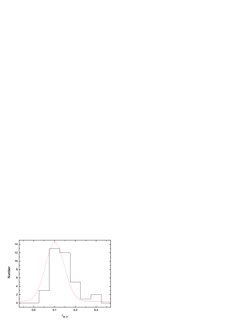
Figure 2: Histogram of the distribution of RSLs for long bursts with a sample of 36 bright pulses. The smooth curve is gaussian function fitted to the distribution, where the mean value is $\mu=0.102$ and the standard deviation is $\sigma=0.045$.

Moreover, we fit the distribution with gaussian function and get $\chi^{2}/dof=1.1$ with $R^{2}=0.97$, which indicates that the distribution of RSLs is consistent with normal distribution. However, the distributions of $FWHM$ and spectral lags (or time intervals) are found to be lognormal instead of normal (see e.g. Mcbreen et al. 2003). In the following, we pay our particular attention to the properties of $\tau_{rel,31}$ that would be studied in very detail as possible.

4.2 The dependence of $\tau_{rel,31}$ on light-curve parameters

To investigate whether $\tau_{rel,31}$ is associated with some parameters of light-curve, we thus list the related parameters in table 1 and make plots of these relations as shown in figure 3.

Table 1: Parameters gained by fit to sample 4 with the current model of this paper

Trigger	$\tau_{rel,31}^{*}$	$\tau_{31}$ (sec)	$FWHM$ (sec)	Asymmetry	$HR_{31}$	$F_{m}$	$t_{m}$ (sec)
1406	0.126$\pm$0.017	1.47$\pm$0.15	9.64$\pm$0.30	0.43$\pm$0.03	0.85	464.09$\pm$2.19	4.47$\pm$0.05
2387	0.127$\pm$0.007	2.43$\pm$0.04	14.57$\pm$0.30	1.38$\pm$0.07	0.95	738.89$\pm$2.03	7.42$\pm$0.03
2665	0.166$\pm$0.014	1.47$\pm$0.10	4.56$\pm$3.40	0.44$\pm$0.51	0.45	327.94$\pm$2.49	3.22$\pm$0.26
3257	0.059$\pm$0.003	1.61$\pm$0.07	12.98$\pm$0.74	0.27$\pm$0.02	1.48	462.97$\pm$2.02	4.16$\pm$0.06
6504	0.105$\pm$0.006	2.02$\pm$0.06	9.78$\pm$1.13	0.36$\pm$0.07	1.49	457.78$\pm$3.15	4.39$\pm$0.11
6625	0.101$\pm$0.04	1.55$\pm$0.19	15.51$\pm$1.24	0.57$\pm$0.08	0.39	338.18$\pm$2.61	9.24$\pm$0.29
7293	0.092$\pm$0.009	1.84$\pm$0.06	12.11$\pm$2.66	0.31$\pm$0.09	1.74	626.78$\pm$2.76	5.32$\pm$0.15
7588	0.149$\pm$0.027	1.14$\pm$0.22	6.56$\pm$0.32	0.56$\pm$0.05	0.60	449.81$\pm$2.63	5.04$\pm$0.06
7648	0.192$\pm$0.036	2.19$\pm$0.30	11.94$\pm$0.60	0.55$\pm$0.05	2.12	305$\pm$4.02	6.89$\pm$0.13

Notes: symbol $\ast$ denotes the relative spectral lags calculated with equations (2) and (3), as shown in table 3.

Figure 3: Correlations between $\tau_{rel,31}$ and other parameters of light-curves such as $\tau_{31}$, $FWHM$, asymmetry, $HR_{31}$, $F_{m}$ and $t_{m}$. These relations will become more tight provided the source # 7648 is excluded from our sub-sample.

The hardness-ratio ($HR_{31}$) here is defined as the ratio of photon counts of channel 3 to channel 1 for pure signal data. The parameters $F_{m}$ and $t_{m}$ as well as their errors are taken from the fit with eq. (1).

For the sake of testing these relations, we take a general linear correlation analysis ([Press et al. 1992]) and derive the correlation coefficients together with probabilities listed in table 2.

Table 2: Linear correlation analysis of figures 3 and 4. Coefficient and probability are abbreviated to coef. and prob. respectively.

Panels		a	b	c	d	e	f
For figure 3	coef.	0.08	-0.48	0.42	-0.04	-0.39	0.03
	prob.	0.84	0.19	0.25	0.92	0.29	0.95
For figure 4	coef.	-0.40	0.32	-0.28	-0.89	-0.87	-0.51
	prob.	0.32	0.43	0.49	0.001	0.002	0.16

In figure 3, unless the data point (# 7648) is removed from these panels (a, d and f), $\tau_{rel,31}$ is evidently uncorrelated with $\tau_{31}$, $HR_{31}$ and $t_{m}$, even though it appears a tendency of reverse correlation between them. We find from the panels (b, c and e) that $\tau_{rel,31}$ shows a positive correlation with asymmetry, while it is reversely correlated with $FWHM$ and $F_{m}$. It demonstrates that the $\tau_{rel,31}$ is very sensitive to $FWHM$ and asymmetry, which suggests that it should be another parameter describing the shape of GRB pulses.

5 Applications and explanations

Encouraged by the special attributes of the $\tau_{rel,31}$, we shall apply this quantity to explore some other potential correlations, so that we can have the opportunity to interpret it in terms of physical significance.

5.1 Detecting relations between $\tau_{rel,31}$ and other physical parameters

First of all, we try to choose the appropriate variables meeting the aim of studies. Since how to determine the energy spectra as well as distances (or energies) is usually considered to be the key issue of understanding the burst phenomenon, we therefore select the relevant parameters such as $\alpha$, $\beta$, $E_{p}$, $z$, $L_{p}$ and $F_{p}$ to correlate with $\tau_{rel,31}$ respectively (see table 3).

Table 3: Parameters for observed and modeled data in sample 4

Trigger	$\tau_{rel,31}^{\ast}$	$\alpha^{a}$	$\beta^{a}$	$E_{p}^{a}$	$z^{b}$	$L_{p}^{b}$	$F_{p}^{a}$
1	2	3	4	5	6	7	8
1406	0.126$\pm$0.017	-1.20$\pm$0.15	-2.89$\pm$0.21	79.43$\pm$21.39	1.91$\pm$0.4	22.8$\pm$10	2.13
2387	0.127$\pm$0.007	-0.03$\pm$0.09	-2.46$\pm$0.03	106.79$\pm$8.00	3.76$\pm$0.4	176$\pm$50	3.58
2665	0.166$\pm$0.014	——	——	——	1.19$\pm$0.11	11$\pm$2	1.91
3257	0.059$\pm$0.003	-0.24$\pm$0.09	-2.79$\pm$0.12	169.2$\pm$16.32	11.97$\pm$1.6	1750$\pm$600	2.62
6504	0.105$\pm$0.006	0.59$\pm$0.26	-2.78$\pm$0.17	120.2$\pm$20.34	1.67$\pm$0.07	40$\pm$4	2.25
6625	0.101$\pm$0.04	-1.18$\pm$0.12	-4.54$\pm$1.76	53.8$\pm$9.31	2.18$\pm$0.4	15.8$\pm$6	1.68
7293	0.092$\pm$0.009	-0.15$\pm$0.12	-2.81$\pm$0.11	151.1$\pm$17.41	8.48$\pm$3	733$\pm$500	2.73
7588	0.149$\pm$0.027	-1.73$\pm$0.38	-2.80$\pm$0.08	12.07$\pm$17.9	1.44$\pm$0.08	7.79$\pm$2.2	2.06
7648	0.192$\pm$0.036	-0.78$\pm$0.26	-2.43$\pm$0.21	146.93$\pm$58.0	0.43 c	0.54$\pm$0.1 d	1.53

Notes.– Redshift (col. 6) and peak luminosity (col. 7) estimated by the $E_{p}-L_{p}$ relation have been borrowed from Yonetoku et al. (2004) due to lack of the information about these sources except for trigger 7648 whose $z$ and $L_{P}$ ($10^{51}$ergs s^-1) is offered by Galama et al. (1999) and Guidorzi et al. (2005) respectively. Note the unit of peak flux ($F_{p}$) is photons $cm^{-2}s^{-1}$.

References.– a. Norris et al. 2005; b. Yonetoku et al. 2004; c. Galama et al. 1999; d. Guidorzi et al. 2005.

It needs to clarify that the redshifts of all sources except # 7648 are borrowed from their estimation by an empirical $E_{p}-L_{p}$ relation instead of direct observations for the absence of their information of the afterglow. The reason for this selection is $E_{p}-L_{p}$ relation looks considerably tighter and more reliable than the relations offered by the previous works ([Yonetoku, et al., 2004]), whereas the spectral parameters ($\alpha$, $\beta$ and $E_{p}$) for # 2665 are unavailable at present.

All the correlations of $\tau_{rel,31}$ with these parameters are shown in figure 4.

Figure 4: Correlations between $\tau_{rel,31}$ and other parameters such as $\alpha$, $\beta$, $E_{p}$, $z$, $L_{p}$ and $F_{p}$. The relations also have the tendency of becoming more tight than before once the source # 7648 is excluded from our sub-sample.

In the same way, we apply the linear correlation analysis to these relations and list the corresponding results in table 2. Figure 4 illustrates all parameters but $\beta$ are reversely correlated with $\tau_{rel,31}$. The high energy spectral index, $\beta$, behaves an otherwise trend of positive correlation with $\tau_{rel,31}$. It has been proposed that $F_{p}$ is often used as an effective indictor of distance to the GRB sources (Lee et al., 2000). The tight relation between $\tau_{rel,31}$ and $F_{p}$ in figure 4(f) shows that $\tau_{rel,31}$ is expected to be a distance indictor.

It is surprisedly found from panels (d) and (e) that $\tau_{rel,31}$ is strongly correlated with $z$ and $L_{p}$ respectively. Accordingly, our attempt in next section is to confirm if $\tau_{rel,31}$ is suitable for an indictor of distance or peak luminosity.

5.2 Redshift and luminosity indicator

As Atteia (2005) points out, whether redshift indictors are good or not is determined by the degree of correlation between redshift and them which are generally combinations of GRB parameters with a small intrinsic scatter. To testify the validity of $\tau_{rel,31}$ as the redshift indicator, we contrast the observed data with the theoretical model in figure 5. Note that the data of panels (a) and (b) are merely a replica of figure 4(d) and (e) correspondingly.

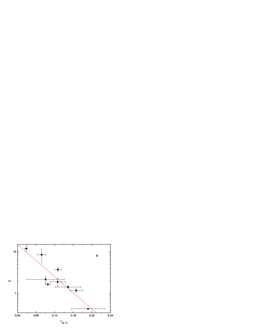
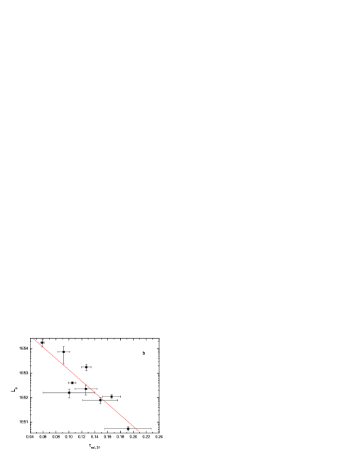
Figure 5: Calibration curves for the relative spectral lags, $\tau_{rel,31}$. Plots of $\tau_{rel,31}$ vs. redshift and peak luminosity can be used to calibrate redshift and/or luminosity indicators. The plots here can be fitted to yield eqs. (13) and (14) (marked with the straight red lines in panels a and b).

From figure 5(a) and (b), the best fits to a linear model are written as

$$\log z\approx 1.56-9.66\tau_{rel,31}$$ (13)

$$\log L_{p}\approx 55.44-23.07\tau_{rel,31}$$ (14)

with spearman rank-order correlation coefficients of -0.88 ($p\sim 1.5\times 10^{-3}$) for the former and -0.83 ($p\sim 5\times 10^{-3}$) for the latter. This indicates the relatively accurate connection between the RSLs and the redshift (or luminosity) does exist. Provided the $\tau_{rel,31}$ is measured, using eqs. (13) and (14) one could precisely estimate redshifts and peak luminosities of those sources without the information of observed spectral lines. From this viewpoint, the quantity $\tau_{rel,31}$ can be regarded as an ideal indicator of redshift and/or luminosity.

Meanwhile, the RSLs might be utilized to constrain the cosmological parameters (say, $\Omega_{m}$, $\Omega_{\lambda}$ and $H_{0}$) in case redshift and luminosity are determined by eqs. (13) and (14) simultaneously. Certainly, the realization of this purpose requires us to eliminate selection effects as possible as we can in advance, not only on observations but also on calculations.

6 Conclusions and discussions

According to above investigations, we could derive the following conclusions: First, the distributions of RSLs are normal and concentrate on the value of 0.1 or so. Second, the RSLs are weakly correlated with $FWHM$, asymmetry, $\alpha$, $\beta$, $E_{p}$, $F_{p}$ and $F_{m}$. While they are uncorrelated with $lags_{31}$, $HR_{31}$ and $t_{m}$. Finally, we find the $\tau_{rel,31}$ is a useful redshift and peak luminosity estimator.

In view of internal shock model, GRBs generally consist of many pulses produced by multiple relativistic shells (or winds) followed by internal shocks due to collision of them as a central engine pumps energy into medium (e.g. Fenimore et al. 1993; Rees & Mészáros  1994). Even so, our action on sample selection doesn’t conflict with the idea of overlapping. For simplicity, we only choose single peaked bursts to construct our sample to make this issue easier to study. Furthermore, the manner of selection can also avoid the contamination of adjacent pulses by overlap, for which could inevitably produce additional errors, owing to selection effects. Under the assumption that these single wide pulses could be produced by the same mechanism (see Piran 1999), our motivation of this selection is advisable. In fact, McMahon et al. (2004) has pointed out the favorite mechanism for producing gamma-ray emission for such single pulse events could be not internal shocks but external shocks (see also Mészáros & Rees 1993; Sari & Piran 1996; Dermer et al. 1999, 2004).

It is usually expected that the gamma-rays come from a relativistically expanding fireball surface with lorentz factor $\Gamma>100$ (e.g. Lithwick et al. 2001). The bulk Lorentz factor increases linearly with radius as long as the fireball is not baryon loaded and not complicated by non-spherical expansion (Eichler et al. 2000) until $\Gamma>1000$ (or $R\geq 10^{16}cm$) (Woods et al., 1995). With Power density spectrum method, Spada et al. (2000) found the curvature time together with the dynamic time will dominate over the radiative cooling time at a distance $R<5\times 10^{14}cm$. Given this case, based on Doppler effects the $FWHM$ has been found to follow $FWHM\propto\Gamma^{-2}$ (Qin et al. 2004). Assuming $\tau\propto\Gamma^{-\omega}$, from figure 3(b) we can deduce that the upper limit of $\omega$ is about 2 which is compatible with $\tau\propto\Gamma^{-1}$ gained by Shen et al. (2005).

In this work we have shown that relative spectral lag can be used as an estimator of redshift and peak luminosity of long GRBs. We note that our conclusion is based on an analysis using nine sources. More accurate and robust results for the analysis would require a larger sample which includes sources with redshifts. Until now the expected indictor of short bursts hasn’t been constructed yet, owing to lack of sufficient sources with the redshift, although redshifts of few sources have been measured by Swift and HETE II and reported recently (see, e.g. Bloom et al. 2005; Hjorth et al. 2005; Berger et al. 2005). The recent observations suggest that short bursts reside at cosmological distances, however, previous investigations showed the spatial population of short GRBs seems to accord with lower redshift sources (e.g. che et al. 1997; Magliocchetti et al. 2003; Tanvir et al. 2005). Therefore, the research on redshift indictor of short bursts is excluded from this work and it still remains at the prenatal stage.