The Limits of Bound Structures in the Accelerating Universe

Abstract

According to the latest evidence, the Universe is entering an era of exponential expansion, where gravitationally bound structures will get disconnected from each other, forming isolated ‘island universes’. In this scenario, we present a theoretical criterion to determine the boundaries of gravitationally bound structures and a physically motivated definition of superclusters as the largest bound structures in the Universe. We use the spherical collapse model self-consistently to obtain an analytical condition for the mean density enclosed by the last bound shell of the structure (2.36 times the critical density in the present Universe, assumed to be flat, with 30 per cent matter and 70 per cent cosmological constant, in agreement with the previous, numerical result of Chiueh and He). $N$-body simulations extended to the future show that this criterion, applied at the present cosmological epoch, defines a sphere that encloses $\approx 99.7$ per cent of the particles that will remain bound to the structure at least until the scale parameter of the Universe is 100 times its present value. On the other hand, $(28\pm 13)$ per cent of the enclosed particles are in fact not bound, so the enclosed mass overestimates the bound mass, in contrast with the previous, less rigorous criterion of, e. g., Busha and collaborators, which gave a more precise mass estimate. We also verify that the spherical collapse model estimate for the radial infall velocity of a shell enclosing a given mean density gives an accurate prediction for the velocity profile of infalling particles, down to very near the centre of the virialized core.

1 Introduction

The evidence for an accelerated expansion of the Universe, initially based on the observations of distant supernovae (Garnavich et al., 1998; Perlmutter et al., 1999) and later strengthened by precise measurements of cosmic microwave background fluctuations (Spergel et al., 2003), has established a new cosmological paradigm based on the presence of a ‘dark energy’ component. In the new scenario, the Universe has recently made a (smooth) transition from a matter-dominated, decelerating stage to a dark-energy dominated, accelerating stage.

In the simplest models, consistent with the observations so far, the dark energy behaves like Einstein’s cosmological constant, providing an always present, constant, positive energy density (and a negative pressure of the same magnitude). As long as the matter density was substantially larger than the dark energy density, it dominated the evolution of the Universe, decelerating the expansion and driving the formation of structures by gravitational instability. When the average matter density fell below that of the dark energy, the latter started accelerating the expansion, and the formation of structure slowed down, as the gravitational forces between matter elements decreased due to their increasing separation. In this stage, structures much denser than the dark energy are not affected by the latter and remain bound, while they separate from each other at an accelerating rate, which does not allow them to join in larger structures. Thus, at the present cosmological time, when the acceleration of the expansion has recently started, the largest bound structures are just forming. In the future evolution of the Universe, their individual, internal properties (such as physical size and density) will not change substantially, but they will grow increasingly isolated, forming ‘island universes’ (e. g., Adams & Laughlin 1997; Chiueh & He 2002; Nagamine & Loeb 2003; Busha et al. 2003).

In the present Universe, these structures have not yet fully formed, virialized, and clearly separated from each other, making it difficult to identify them unambiguously. Superclusters, the largest structures identifiable in the present Universe, have generally been defined by more or less arbitrary criteria (e. g., Quintana, Carrasco & Reisenegger 2000; Einasto et al. 2001, 2003a, 2003b; Proust et al. 2005). Here, we address the question of how to decide whether such a structure will remain gravitationally bound in the future evolution of the Universe, forming an island universe, and propose to use this criterion as a physical definition of superclusters.

We study the well-known spherical collapse model in the presence of a cosmological constant, with the aim of obtaining a useful method to study structure behavior in our Universe. The spherical collapse model considers a spherically symmetric mass distribution, where spherical shells expand or collapse into the centre of the structure in a purely radial motion and without crossing each other. Specifically, we study the density that needs to be enclosed by a spherical shell at a given cosmological epoch in order to stay gravitationally attached to the overdense region within in a distant future, dominated by a cosmological constant.

Previously, Lokas & Hoffman (2002) gave an approximate criterion for this density, assuming that the shell in question initially expands with the Hubble flow (without retardation from the enclosed over-density) and present density evolution curves considering different cosmologies. Chiueh & He (2002), on the other hand, solved the spherical collapse equations numerically, both with a cosmological constant and with a more general form of dark energy (with a constant ‘equation-of-state parameter’ $w_{q}$), obtaining a self-consistent, theoretical criterion for the mean density enclosed in the last gravitationally bound or ‘critical’ shell. Both Nagamine & Loeb (2003) and Busha et al. (2003) studied the future evolution of structures numerically, contrasting the extension of bound structures in a distant future (at scale parameter $a=166$ and $a=100$, respectively) with the criterion of Lokas & Hoffman (2002) applied at the present time ($a=1$). While Nagamine & Loeb (2003) focused on the evolution of specific structures in our local Universe (the Local Group, the Virgo cluster, and other nearby structures), Busha et al. (2003) followed the internal density and velocity structures of generic, bound objects as they evolve, a subject taken up again by the same authors more recently (Busha et al., 2005).

We stress that, among the previous work cited above, only Chiueh & He (2002) used the spherical collapse model self-consistently in order to obtain the density criterion for the last bound shell, whereas all the other papers rely on the incorrect assumption that the shell expands with the Hubble flow at the initial epoch (taken to be the present time, both by Nagamine & Loeb 2003 and Busha et al. 2003). On the other hand, Chiueh & He (2002) did not perform numerical simulations of the future evolution of structure in order to test the accuracy of their result in a non-ideal situation and in order to study the details of the evolution of bound objects, as the other authors did. In this work, we attempt to bring together and extend the best parts of the previous work, by a self-consistent application of the spherical collapse model (supplemented by a new, analytic equation for the mean density of a marginally bound sphere) and a comparison of its predictions to $N$-body simulations of the future Universe.

In section 2, we review the spherical collapse model, deriving an analytical solution for the spherical collapse equations. Our solution, which agrees with the numerical result of Chiueh & He (2002), relates the critical shell’s overdensity with the value of the dimensionless parameter $\Omega_{\Lambda}(t)=\Lambda/[3H(t)^{2}]$ (where $\Lambda$ is the cosmological constant and $H(t)$ is the Hubble parameter), so we are able to evaluate the criterion at any time $t$ of the evolution of the Universe. We also obtain numerical solutions for the velocities of non-critical shells in the present Universe ($\Omega_{\Lambda}=0.7$).

In sections 3 through 5, we compare the theoretical results with simulated data, studying the quality of the criterion and its applicability to real-world observations. As in Nagamine & Loeb (2003) and Busha et al. (2003), $N$-body simulations were run until the very late future ($a=100$), in order to reproduce the final configuration of bound structures. We find that the rigorous density criterion proposed by us (in agreement with Chiueh & He 2002) gives a good upper bound to the size of the bound structure, as it encloses $\approx 99.7$ per cent of the bound particles. On the other hand, it also encloses a substantial number of unbound particles, and therefore does not perform as well as the criterion of Lokas & Hoffman (2002) (used by Nagamine & Loeb 2003 and Busha et al. 2003) for the purpose of estimating the bound mass. We also show that the spherical collapse model is quite accurate in predicting (as a function of the enclosed mean density) the radial velocity of the stream of particles falling into a bound structure for the first time, down to the very centre of the structure.

2 Spherical collapse model

A straightforward approach to the evolution of structure is obtained by considering a spherical distribution where all layers expand or contract with only radial motions and without crossing each other. The later ensures that the enclosed mass in every shell stays constant throughout its whole evolution, being the only parameter other than initial conditions to determine its behavior. The model is more accurate during the expansion phase, but becomes unrealistic after contraction begins, because the instability in angular momentum during this phase causes non-radial motions and finally virialization. In our analysis, we are going to leave aside this warning and check the accuracy of the model in the contraction phase using comparison with simulations.

Our analysis will be based on Newtonian Mechanics, which, according to Lemaître (1931), is a limiting approximation to general relativity, valid no matter what is happening in distant parts of the Universe. The Newtonian approximation is accurate in a region small compared to the Hubble length $c/H$ and large compared to the Schwarzschild radii of any collapsed objects. For more details, see Peebles (1980).

Under the assumption that the total energy will be conserved during the shell’s expansion and later contraction, the evolution of a spherical shell enclosing a spherically symmetric mass distribution is given by the energy equation (Peebles, 1980):

$$E={1\over 2}\left(dr\over dt\right)^{2}-\frac{GM}{r}-\frac{\Lambda}{6}r^{2},$$ (1)

where $r$ is the shell’s radius, $M$ is the total mass enclosed by it, $\Lambda$ is the cosmological constant and $E$ is the total energy per unit mass of the shell.

This equation can be simplified by introducing the following dimensionless variables:

$$\widetilde{r}=\left(\frac{\Lambda}{3GM}\right)^{1/3}r,\\$$ (2)

$$\widetilde{t}=\left(\frac{\Lambda}{3}\right)^{1/2}t.\\$$ (3)

Therefore, the equation may be written

$$\widetilde{E}={1\over 2}\left(d\widetilde{r}\over d\widetilde{t}\right)^{2}-\frac{1}{\widetilde{r}}-\frac{\widetilde{r}^{2}}{2},$$ (4)

where

$$\widetilde{E}=E\left(\frac{G^{2}M^{2}\Lambda}{3}\right)^{-1/3}.$$ (5)

Fixing $M$ and considering that there is no shell crossing, this equation describes the time evolution of a single shell. $\widetilde{E}$ is the dimensionless energy that describes every shell of the distribution, merging with the background’s mean density when $\widetilde{E}=0$, shell that will expand with the Hubble flow.

2.1 The critical shell and turn-around radius

We are looking for a critical shell that will stay at the limit between expanding for ever or re-collapsing into the structure. To find the critical energy for such a shell, we define a potential energy to be maximized as

$$\widetilde{V}=-\frac{1}{\widetilde{r}}-\frac{\widetilde{r}^{2}}{2}.$$ (6)

The maximum of this potential occurs at $\widetilde{r}^{*}=1$, so $\widetilde{E}^{*}\equiv\widetilde{V}\left(\widetilde{r}^{*}\right)=-\frac{3}{2}$ is the maximum possible energy for a shell to remain attached to the structure. The maximum radius for a critical shell is

$$r_{\mathrm{max}}\equiv\left(\frac{3GM}{\Lambda}\right)^{1/3},$$ (7)

so we can reinterpret the normalized radius $\widetilde{r}$ as

$$\widetilde{r}\equiv\frac{r}{r_{\mathrm{max}}}.$$ (8)

2.2 Connection with the background model

Assuming a flat universe with cosmological constant, the age of the Universe (time since the Big Bang, written in our dimensionless variables) may be related to the vacuum energy density parameter (Peebles, 1980),

$$\Omega_{\Lambda}\equiv{\Lambda\over 3H^{2}}=\tanh^{2}(3\widetilde{t}/2),$$ (9)

showing that $\Omega_{\Lambda}$ increases monotonically in time, and can therefore be used as a surrogate time variable, in terms of which we will describe the evolution of bound or critical (marginally bound) spherical shells.

Integrating equation (4) from the beginning of time ($\widetilde{r}=0$) till the current radius of a given shell ($\widetilde{r}=\widetilde{r}_{0}$), we get

$$\widetilde{t}_{0}=\int^{\widetilde{r}_{0}}_{0}\frac{\sqrt{\widetilde{r}}d\widetilde{r}}{\sqrt{\widetilde{r}^{3}+2\widetilde{E}\widetilde{r}+2}}.$$ (10)

In the particular case of a critical shell ($\widetilde{E}=\widetilde{E}^{*}=-\frac{3}{2}$), the denominator of equation (10) can be factorized, yielding

$$\widetilde{t}_{0}=\int^{\widetilde{r}_{0}}_{0}\frac{\sqrt{\widetilde{r}}d\widetilde{r}}{\left(1-\widetilde{r}\right)\sqrt{\widetilde{r}+2}}.$$ (11)

The integral can be done analytically, with the result

$$\widetilde{t_{0}}=\frac{1}{2\sqrt{3}}\ln\left[\frac{1+2\widetilde{r_{0}}+\sqrt{3\widetilde{r_{0}}\left(\widetilde{r_{0}}+2\right)}}{1+2\widetilde{r_{0}}-\sqrt{3\widetilde{r_{0}}\left(\widetilde{r_{0}}+2\right)}}\right]$$ (12)

$$-\ln\left[1+\widetilde{r_{0}}+\sqrt{\widetilde{r_{0}}\left(\widetilde{r_{0}}+2\right)}\right].$$

Notice that $\widetilde{r}_{0}$ can be chosen at any ‘current’ time, so equation (12) can be generalized to any time by simply dropping subscript 0. From now on, we will use the subscript ‘cs’ to indicate that we are referring to a critical shell.

Replacing eq. (12) in eq.(9), and introducing a new variable

$$\chi\left(\widetilde{r}_{\mathrm{cs}}\right)\equiv\left[\frac{1+2\widetilde{r}_{\mathrm{cs}}+\sqrt{3\widetilde{r}_{\mathrm{cs}}\left(\widetilde{r}_{\mathrm{cs}}+2\right)}}{1+2\widetilde{r}_{\mathrm{cs}}-\sqrt{3\widetilde{r}_{\mathrm{cs}}\left(\widetilde{r}_{\mathrm{cs}}+2\right)}}\right]^{\frac{\sqrt{3}}{2}}$$ (13)

$$\times\left(1+\widetilde{r}_{\mathrm{cs}}+\sqrt{\widetilde{r}_{\mathrm{cs}}\left(\widetilde{r}_{\mathrm{cs}}+2\right)}\right)^{-3},$$

we can write the relation between $\Omega_{\Lambda}$ (and therefore cosmological time) and $\widetilde{r}_{\mathrm{cs}}$ as

$$\Omega_{\Lambda}\left(\widetilde{r}_{\mathrm{cs}}\right)=\left[\frac{\chi\left(\widetilde{r}_{\mathrm{cs}}\right)-1}{\chi\left(\widetilde{r}_{\mathrm{cs}}\right)+1}\right]^{2}.$$ (14)

As expected (see Fig. LABEL:fig:Om_r), $\widetilde{r}_{\mathrm{cs}}$ grows with $\Omega_{\Lambda}$ as $\Omega_{\Lambda}$ grows with time, and will converge to its maximum radius when $t\rightarrow\infty$.

Inversely, evaluating equation (14) at our preferred cosmology ($\Omega_{\mathrm{m}}=0.3$, $\Omega_{\Lambda}=0.7$), we obtain that current critical shells should have $\widetilde{r}_{\mathrm{cs}}=0.84$, which means that their present radius is 84 per cent of the maximum radius they will reach as $t\rightarrow\infty$.

2.3 Conditions for a critical shell

For practical applications, it is convenient to express the critical condition as the minimum enclosed mean density needed by a shell to stay bound to the central gravitational attractor. The critical density of the Universe (in the flat model, also the average total density, including matter and vacuum energy) is

$$\rho_{\mathrm{c}}=\frac{3H^{2}}{8\pi G},$$ (15)

and the average mass density enclosed by a given shell is

$$\bar{\rho}_{\mathrm{m}}^{\mathrm{s}}=\frac{3M}{4\pi r^{3}}.$$ (16)

Defining the mass density parameter for the shell,

$$\Omega_{\mathrm{s}}\equiv\frac{\bar{\rho}_{\mathrm{m}}^{\mathrm{s}}}{\rho_{\mathrm{c}}}=\frac{2\Omega_{\Lambda}}{\widetilde{r}^{3}},$$ (17)

the condition for the shell to be bound is

$$\Omega_{\mathrm{s}}\geq\Omega_{\mathrm{cs}}=\frac{2\Omega_{\Lambda}}{\widetilde{r}_{\mathrm{cs}}^{3}}=2.36,$$ (18)

where we have evaluated equation (14) at the present value of $\Omega_{\Lambda}=0.7$. This represents the present density contrast inside the last shell that will eventually stop its growth at the end of times. This result was first obtained by Chiueh & He (2002), using numerical methods, but now we confirm this result with an analytical solution. In the same way, evaluating at $\Omega_{\Lambda}=1$ ($t\rightarrow\infty$) we obtain the asymptotic critical density contrast condition $\Omega_{\mathrm{cs},\infty}=2$.

Fig. LABEL:fig:F shows the density parameter $\Omega_{\mathrm{cs}}$ as a function of $\Omega_{\Lambda}$ and $\widetilde{r}_{\mathrm{cs}}$ using equation (14) or its inverse. It is curious that the curve shows a single maximum at $\Omega_{\Lambda}=0.72$, very close to the measured value of $\Omega_{\Lambda}$ today. Considering that $\Omega_{\Lambda}$ can be taken as a function of time, this means that we are living in the era when the ratio between mass density inside a critical shell and the critical density of the Universe is very nearly at its maximum.

For observational purposes, it is more interesting to know the ratio between the mass density enclosed by the critical shell, $\bar{\rho}^{\mathrm{s}}_{\mathrm{m}}$, and that of the background, $\rho^{\mathrm{b}}_{\mathrm{m}}$. Using equation (17), we obtain that

$$\frac{\bar{\rho}^{\mathrm{s}}_{\mathrm{m}}}{\rho^{\mathrm{b}}_{\mathrm{m}}}=\frac{\bar{\rho}^{\mathrm{s}}_{\mathrm{m}}}{\rho_{\mathrm{c}}\left(1-\Omega_{\Lambda}\right)}=\frac{\Omega_{\mathrm{cs}}}{1-\Omega_{\Lambda}}.$$ (19)

which, evaluated for $\Omega_{\Lambda}=0.7$, yields

$$\frac{\bar{\rho}^{\mathrm{s}}_{\mathrm{m}}}{\rho^{\mathrm{b}}_{\mathrm{m}}}=7.88.$$

In the notation of Busha et al. (2003), considering only the excess density with respect to the background ($M_{\mathrm{obj}}=M-M_{\mathrm{b}}$, where $M_{\mathrm{b}}$ is the amount of mass contained in an equivalent sphere with background density) and writing the present value of the Hubble parameter as $H_{0}=70~{}h_{70}\mathrm{km~{}s^{-1}~{}Mpc^{-1}}$, we rewrite the criterion as

$$\frac{M_{\mathrm{obj}}}{10^{12}M_{\odot}}\geq 1.18~{}h_{70}^{2}\left(\frac{r_{0}}{1\hbox{$\rm\thinspace Mpc$}}\right)^{3}.$$ (20)

This is a less restrictive condition than the one proposed by Busha et al. (2003), which is

$$\frac{M_{\mathrm{obj}}}{10^{12}M_{\odot}}\geq 3~{}h_{70}^{2}\left(\frac{r_{0}}{1\hbox{$\rm\thinspace Mpc$}}\right)^{3},$$ (21)

or, equivalently, $\Omega_{\mathrm{s}}\geq 5.56$ (also equivalent to the overdensity criterion given by Nagamine & Loeb 2003, based on the formalism of Lokas & Hoffman 2002). This result was expected, since the criterion of Busha et al. (2003) was obtained under the assumption that the test particles, placed on the critical shell today, move with the Hubble flow. As this is not really true, they free that parameter (velocity of particles on the critical shell today) and do an empirical test to observe the real behavior of particles evolved till $a=100$. They obtain a corrected result which is closer to their initial result than to ours, always setting a higher constraint to the critical shell density. A probable reason for this difference is that our result is a completely theoretical approach based on the spherical collapse model (only radial motions), but in real life objects usually obtain angular momentum caused by tidal forces, which will tend to detach objects from the structure, strengthening the binding condition. This discussion will be resumed later, in relation to the results of our simulations.

2.4 Velocities of shells

In order to work with shell velocities, it is convenient to refer the radial velocities to the Hubble flow, so we introduce the parameter $A$, defined as in Busha et al. (2003),

$$A\left(\Omega_{\Lambda}\right)\equiv\left({1\over H_{0}r}{dr\over dt}\right)^{2}.$$ (22)

For a critical shell, we can use equation (4) to write this in terms of $\Omega_{\Lambda}$ as

$$A_{\mathrm{cs}}\left(\Omega_{\Lambda}\right)=\Omega_{\Lambda}\left[1-\frac{3}{\widetilde{r}^{2}\left(\Omega_{\Lambda}\right)}+\frac{2}{\widetilde{r}^{3}\left(\Omega_{\Lambda}\right)}\right].$$ (23)

Evaluating at $\Omega_{\Lambda}=0.7$, we obtain that the present velocity parameter for a critical shell is $A_{\mathrm{cs}}=8.63\times 10^{-2}$, showing that the shell has been slowed down substantially with respect to the Hubble flow.

To study the velocity profile of a mass overdensity, it is convenient to relate the energy of an arbitrary shell to its normalized radius, characterized by the present value of $\Omega_{\Lambda}$. Unfortunately, the energy integral has no analytical solution for $\widetilde{E}\neq\widetilde{E}^{*}$, so this relation can only be obtained numerically. Fixing the value of $\Omega_{\Lambda}$ to 0.7, in order to represent the present universe, we obtain the current normalized time $\widetilde{t}_{0}=0.81$. Then, we numerically integrate equation (10) for every possible value of $\widetilde{E}$ from zero till some value of $\widetilde{r}$ that satisfies the time constraint. Now using equation (17), we arrive at the more useful numerical function $\widetilde{E}(\Omega_{\mathrm{s}};\Omega_{\Lambda})$, which is best shown in Fig. LABEL:fig:r_E.

Expressing the velocity parameter $A$ in terms of an arbitrary normalized energy $\widetilde{E}(\Omega_{\mathrm{s}};\Omega_{\Lambda})$, for a fixed value $\Omega_{\Lambda}$, we obtain

$$A=\Omega_{\Lambda}+\Omega_{\mathrm{s}}+\widetilde{E}(\Omega_{\mathrm{s}};\Omega_{\Lambda})\left(2\Omega_{\Lambda}\Omega_{\mathrm{s}}^{2}\right)^{1/3}.$$ (24)

In Fig. LABEL:fig:A_OmegaM, we observe that $A(\Omega_{\mathrm{s}})$ is zero when $\Omega_{\mathrm{s}}=\Omega_{\mathrm{s,ta}}$, the density parameter corresponding to the turn-around radius. When solving for the radial velocity, it is important to notice that shells with $\Omega_{\mathrm{s}}>\Omega_{\mathrm{s,ta}}$ contract, while shells with $\Omega_{\mathrm{s}}<\Omega_{\mathrm{s,ta}}$ expand. For a universe with $\Omega_{\Lambda}=0.7$, $\Omega_{\mathrm{s,ta}}=3.66$.

3 Numerical simulations

We simulate one cosmological model, assuming a standard flat Lambda Cold Dark Matter ($\Lambda$CDM) Universe. The current cosmological parameters in the simulation are $\Omega_{\mathrm{m},0}=0.3$, $\Omega_{\Lambda,0}=0.7$ and $h=0.7$, where the Hubble parameter $H_{0}=100h$ km s^-1Mpc^-1. The normalization of the power spectrum is $\sigma_{8}=1$. The box has a side length of 100$h^{-1}$Mpc and contains 128³ dark matter particles of mass $m_{\mathrm{DM}}=3.97\times 10^{10}h^{-1}M_{\odot}$. The simulation was evolved from $a=0.02$ (redshift $z=49$) to $a=100$. The Plummer-equivalent gravitational softening was set to $\epsilon_{\mathrm{Pl}}=15$ $\thinspace h^{-1}\hbox{$\rm\thinspace kpc$}$ (physical units) from $a=1/3$ to $a=100$, while it was taken to be fixed in comoving units at higher redshift.

The run was performed with the massive parallel tree $N$-body/SPH code GADGET (Springel, Yoshida & White, 2001). This is a TREESPH code where the dark matter particles are evolved using a tree-code, while the collisional gas is followed using the SPH approach. Here, we used the new improved GADGET2, kindly provided by Volker Springel (Springel, 2005), which is more memory-efficient, offers better time-stepping for collisionless dynamics, and is substantially faster than the original version. The initial conditions were established by the code of van de Weygaert & Bertschinger (1996).

We took snapshots at the present time ($a=1$) and in the far future ($a=100$), assuming that in late epochs the structure evolution will decrease significantly, so no major changes will be seen from then on. The identification of structures was done using a friend-of-friends code to identify the initial candidates and later extracting the structures to produce a reduced catalog for our study.

4 Application of binding criteria to simulation data

We identified 22 mass concentrations with masses greater than $10^{14}~{}\hbox{$\thinspace h_{70}^{-1}\hbox{${\rm\thinspace M}_{\odot}$}$}$, from which we selected 11 that were away from the box boundaries in order to do our analysis. The same identification was done in the future frame ($a=100$), obtaining the final state for the structures identified at $a=1$. We were able to follow particles from the present till the late future frame, so we could exactly determine the fate of every particle.

In order to apply the density criterion for gravitational binding, we first identified the densest core of the structure. For this, we chose a centre and found the radius where the mean inner density was 300 times the critical density of the Universe (chosen to identify a dense, virialized core that would be clearly detectable in observations). We then re-centred the sphere to its centre of mass. We repeated this procedure until the centre of mass matched the geometric centre of the sphere. Once the centre was fixed, we calculated the density parameter $\Omega_{\mathrm{s}}$ of concentric spheres with increasing radius until the condition $\Omega_{\mathrm{s}}<\Omega_{\mathrm{cs}}=2.36$ stopped being satisfied. We called the identified radius $r_{\mathrm{c}}$. (The radii and masses of these structures are plotted in Fig. LABEL:fig:MvsR). The same identification was done at $a=100$, with the critical condition $\Omega_{\mathrm{s}}<\Omega_{\mathrm{cs},\infty}=2$. In order to contrast our results, we applied the criterion of Busha et al. (2003) at $a=1$, which is given by $\Omega_{\mathrm{s}}<\Omega_{\mathrm{cs,B}}=5.56$. We called the identified radius $r_{B}$.

A critical part of the analysis is to have an acceptable criterion to determine whether a particle is bound to the overdense structure or not. As illustrated in Fig. LABEL:fig:vr_100, the theoretical criterion at $a=100$ gives a very intuitive result, placed at the end of the virialized region, almost exactly where the lower envelope of the radial velocities crosses zero. In other words, $\Omega_{\mathrm{cs},\infty}$ coincides with the last radius where objects with negative radial velocity can be found. At that point, only a few particles will be able to escape, so we can say that the criterion at $a=100$ is adequate to determine the limits of bound structures in the distant future universe. A very similar figure, as well as a detailed discussion of how the velocity distribution evolves to this state, was recently given by Busha et al. (2005).

Finally, we classified particles in four categories: particles that fall inside the theoretical critical shell at $a=1$ and $a=100$; particles that fall inside the critical shell at $a=1$ but do not at $a=100$; particles that fall outside the critical shell at $a=1$ but inside at $a=100$ and particles that fall outside in both cases. This categorization lets us visualize the quality of our estimation, clearly separating particles according to their real fate, and permitting us to calculate statistical indicators useful to produce the desired error estimations. As expected, not every object presented a very ‘spherical’ distribution at $a=1$, and this affected how well data were fitted by the spherical model. For this reason, we based our qualitative analysis on the ‘best’ objects, but we kept all of them when doing statistics.

5 Comparison between theory and simulated data

The spherical model predicts a purely radial motion of particles towards the centre. This is clearly not the case in the real world, where objects are affected by multiple and complicated tidal forces produced by other objects in their surroundings all along their evolution. In fact, objects present a velocity dispersion that is greatest in the virialized cores of galaxy clusters. The presence of other overdensities surrounding the main attractor alters the motion, pushing particles away from their radial trajectories. For this reason, we expect the spherical model to give a lower bound on the radial velocities at a given radius (with outward-pointing velocities taken as positive) and an upper limit for the radius of critical shells.

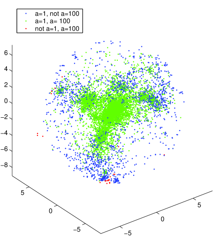
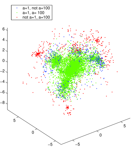
Figure 7: Spatial distribution of particles in object no. 1 (see Table 1) with colours depending on our criterion (left-hand panel), or on that of Busha et al. (2003) (right-hand panel). Blue: they satisfy the criterion at $a=1$, but not at $a=100$, Green: they satisfy the criterion at $a=1$ and $a=100$, Red: they do not satisfy the criterion at $a=1$, but they do at $a=100$. Particles that do not satisfy the criterion at either $a=1$ or $a=100$ are not shown.

To test the performance of the criterion, we first selected all the particles that were bound at $a=100$ and ‘marked’ them, so they could be recognized at $a=1$, as shown for the most massive structure in Fig. 7. Later, we selected all the particles that satisfied the criterion at $a=1$ and produced four statistical indicators: $A$, the fraction of all particles selected by the criterion as bound at $a=1$ that were not selected at $a=100$; $B$, the fraction of all particles selected at $a=1$ that were also selected at $a=100$; $C$, the ratio of the number of particles not selected at $a=1$ but selected at $a=100$, to the total number of selected particles at $a=1$ and $D$, the ratio of the mass still bound at $a=100$ to the mass selected at $a=1$. Results were averaged over all objects to obtain a single indicator. Results for our criterion are shown in Table 1 and for that of Busha et al. (2003) in Table 2.

Table 1: Quantitative results after application of our theoretical criterion to 11 objects from the simulation. Columns: (1) index of the object; (2) $A$, particles selected by the criterion as bound at $a=1$ but not at $a=100$, as fraction of all particles selected at $a=1$; (3) $B$, particles selected at $a=1$ and $a=100$, as fraction of all particles selected at $a=1$ (note $A+B=100$ per cent); (4) $C$, ratio of the number of particles not selected at $a=1$ but selected at $a=100$, to the total number of selected particles at $a=1$; (5) $M(a=1)$, total mass selected inside the critical radius at $a=1$; (6) $M(a=100)$ total mass selected inside the critical radius at $a=100$ and (7) $D=M(a=100)/M(a=1).$

Object	$A$	$B$	$C$	$M(a=1)$	$M(a=100)$	$D$
no.	[per cent]	[per cent]	[per cent]	$[10^{14}\hbox{$\thinspace h_{70}^{-1}\hbox{${\rm\thinspace M}_{\odot}$}$}]$	$[10^{14}\hbox{$\thinspace h_{70}^{-1}\hbox{${\rm\thinspace M}_{\odot}$}$}]$	[per cent]
1	16.8	83.2	0.20	7.63	6.36	83.4
2	18.3	81.7	0.22	6.46	5.29	81.9
3	18.7	81.3	0.50	5.76	4.71	81.8
4	37.9	62.1	0.04	6.66	4.14	62.1
5	25.4	74.6	0.62	5.41	4.07	75.2
6	51.6	48.4	0.21	6.64	3.23	48.6
7	50.5	49.5	0.06	5.96	2.96	49.6
8	26.7	73.3	0.07	3.34	2.45	73.3
9	17.2	82.8	0.67	2.88	2.40	83.4
10	17.6	82.4	0.09	2.45	2.02	82.4
11	29.6	70.4	0.22	2.07	1.46	70.6
Mean	28.2	71.8	0.26			72.0
Std. dev.	13.0	13.0	0.23			13.1

Table 2: Quantitative results after application of the criterion of Busha et al. (2003) to 11 objects from the simulation. The variables are defined as in Table 1.

Object	$A$	$B$	$C$	$M(a=1)$	$M(a=100)$	$D$
no.	[per cent]	[per cent]	[per cent]	$[10^{14}\hbox{$\thinspace h_{70}^{-1}\hbox{${\rm\thinspace M}_{\odot}$}$}]$	$[10^{14}\hbox{$\thinspace h_{70}^{-1}\hbox{${\rm\thinspace M}_{\odot}$}$}]$	[per cent]
1	7.4	92.6	9.3	6.24	6.36	101.9
2	8.7	91.3	6.0	5.44	5.29	97.2
3	7.1	92.9	27.7	3.91	4.71	120.5
4	10.8	89.2	2.7	4.51	4.14	91.8
5	8.4	91.6	17.2	3.74	4.07	108.8
6	10.2	89.8	42.8	2.43	3.23	132.6
7	15.8	84.2	5.9	3.28	2.96	90.1
8	16.3	83.7	7.2	2.69	2.45	90.8
9	3.7	96.3	18.8	2.09	2.40	115.2
10	5.9	94.1	4.8	2.04	2.02	98.9
11	14.9	85.1	4.3	1.64	1.46	89.4
Mean	9.9	90.1	13.3			103.4
Std. dev.	4.2	4.2	12.4			14.3

We observe that the purely theoretical criterion is good to determine the exterior limit of the object since only very few particles (0.26 per cent of the particles that satisfied the criterion at $a=1$) that are outside the criterion today will fall inside in the late future. In contrast, a significant number of particles (28 per cent of the particles under the criterion) were predicted to belong, but finally escaped. Finally, a large number of particles (72 per cent of the particles under the criterion) were correctly predicted to belong to the overdensity. Based on this result, we can assert that the theoretical criterion is adequate to give an upper bound to the structure extension, but overestimates its mass, which turns out to be about 72 per cent of the predicted mass.

With the criterion of Busha et al. (2003), a greater number of particles (13 per cent of the particles under the criterion at $a=1$) fell outside the criterion today, but ended up inside the object. In contrast, a smaller number of particles (10 per cent of the particles that satisfied the criterion) were incorrectly predicted to belong, while a very large number of particles (90 per cent of the particles under the criterion) were correctly recognized. Thus, although it is based on an inconsistent application of the spherical collapse model, it happens to give a better estimate for the final object mass, underestimating it by only $\approx 3$ per cent.

It is also important to add that objects 6 and 7 had very complex cores, being separated into two main concentrations. Of these, we selected the most massive as the centre of the spherical analysis. We kept our selection criterion for the centre, under the assumption that it should be easier to detect the centre of the most massive concentration when dealing with real observations.

5.1 Radial velocity predictions

An important prediction of the spherical collapse model is the radial velocity of shells falling toward the gravitational attractor. The velocity information is contained in the velocity parameter $A$, which depends only on the mass energy density inside the shell, $\Omega_{\mathrm{s}}$. This can be calculated numerically for every shell of the studied objects, yielding the desired radial velocity.

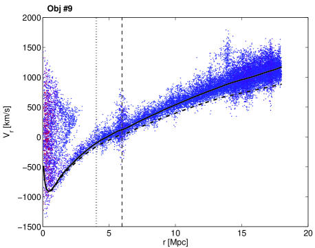
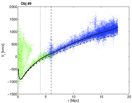
Figure 8: Radial velocities as a function of radius for a mass overdensity at $a=1$ for object no. 9. Left-hand panel: colours as a function of tangential velocities. Red dots indicate more radial velocity and bluer ones less radial velocity. Right-hand panel: colours depending on final fate of particles: green particles remain bound to the structure, blue particles do not. The vertical dashed line shows the radius where $\Omega_{\mathrm{s}}<\Omega_{\mathrm{cs}}=2.36$, while the vertical dotted line indicates the critical radius according to Busha et al. (2003). The solid curve is the theoretical approximation considering a flat universe with a cosmological constant. The dashed curve is the theoretical approximation considering a universe without cosmological constant and $\Omega_{M}=0.3$.

In Fig. 8, we plot the radial velocity against radius, together with the theoretical approximation using the spherical collapse model with and without cosmological constant (see Reisenegger et al. 2000, for details about the approximation using the spherical collapse model without a cosmological constant). For this analysis, we chose object no.9 because it presented a clear stream of infalling particles flowing at high speed to the object’s core, cleanly separated from the virialized particles and from particles currently outflowing after a first pass through the centre, forming an empty space reaching as close as $2\hbox{$\rm\thinspace Mpc$}$ from the core. Other objects presented similar overall characteristics, but they did not show such a clear separation between infalling particles and virialized ones, probably as a result of earlier virialization or the presence of substructure. We observe that the spherical model with cosmological constant is accurate to determine the mean radial velocity of the infalling part of the cluster particles, correcting the underestimate of radial velocities at large radius seen in the spherical model without cosmological constant.

An important observation is that the theoretical velocity profile follows the infalling particles deep into the core of the structure, where virialization effects are very important. This result, which was confirmed on every object we studied, tells us that the spherical collapse model produces robust predictions of the negative velocity envelope profile even in highly virialized cores. The decrease on the predicted velocity very near to the centre is probably due to the poor resolution of the simulation and to extreme virialization effects.

5.2 Perturbations from spherical collapse

In the previous analyses, we observe that there is a considerable number of particles that escape from the structure, contradicting the theoretical prediction. There are two main candidates to be responsible for this: one is the appearance of tangential velocities during the contraction, which is also responsible for virialization, the other is the influence of external structures which can act as gravitational attractor on external shells. A simple test is to plot tangential velocities as a function of radius. We would expect that if there is a clear relation between angular momentum and failure of the criterion, we would find that particles that contradict the criterion would have greater tangential velocities than particles that verify the criterion. This was done for object no. 9 and results are shown in Fig. 9.

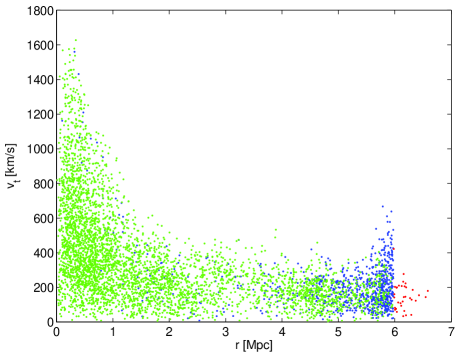
Figure 9: Tangential velocities as a function of radius for object no. 9 at $a=1$. Colors depend on the final fate of particles, as given in Fig. 7.

As seen in Fig. 9, and as we observed in all other objects, there is no clear relation between tangential velocity and probability of escaping. This result is solid enough to say that angular momentum is not the main reason for the failure of the criterion, so the hypothesis of external attractors seems more acceptable. Just as a follow-up observation, we can see in Fig. 7 that the particles incorrectly identified as bound by our criterion (blue) are commonly related to denser regions outside and close to the critical shell, while the particles incorrectly identified as unbound (red) are close to mass concentrations inside the critical shell that finally fall to the centre. We conclude that the failure of the method is mainly caused by external overdensities or perturbations from the spherical distribution of the studied object.

6 Conclusions

We have presented a complete discussion of the model of spherical, gravitational collapse in a flat Universe with a cosmological constant, applied to estimate the size and mass of bound structures in the Universe. Within this model, we derive an exact, analytical equation for the minimum enclosed mass density required for a shell to remain bound until a very distant future. For the present cosmological parameters ($\Omega_{\mathrm{m}}=0.3$, $\Omega_{\Lambda}=0.7$), this minimum density is 2.36 times the critical density of the Universe, as found numerically by Chiueh & He (2002). This suggests a both physical and practical criterion for the limits of a bound structure, such as the previously fairly ill-defined superclusters of galaxies, as the shell enclosing precisely this density.

The application of the model to simulated data gave encouraging results, demonstrating first its great ability to find the limits of structure in the late future, and, second, giving reasonably good results in determining the limits of bound structures at the present epoch. On average, 72 per cent of the mass enclosed by the estimated radius is really bound to the structure, while the mass that, although bound to the structure, is not enclosed by the radius is only a 0.3 per cent. For the less rigorous criterion of Busha et al. (2003) and other authors, these numbers are 90 and 13 per cent, giving a substantially better estimate for the object’s final mass. Thus, the sphere defined by our criterion is an outer envelope enclosing all the particles bound to the structure (and quite a few more), while that of Busha et al. (2003) encloses as much mass as will remain bound to the distant future (leaving about as many bound particles outside as unbound ones inside).

The spherical collapse model also defines a radial velocity profile that we will use in our next paper (Dünner et al., in preparation) to find the shape of these structures in redshift space, in order to make them identifiable in redshift surveys. This profile was found in the simulations to fit the observed velocity profile of infalling particles well down to deep inside the virialized radius. Thus, even though the spherical collapse model is intrinsically unstable for contracting shells, it still gives a reliable performance in a broad set of radii. Moreover, we observed that the greatest perturbations from the theoretical model were produced by gravitational perturbations by external structures or by substructures falling into the external shells of the structure.

’

References

- Adams & Laughlin (1997) Adams F. C., Laughlin G., 1997, Rev. Mod. Phys., 69, 337
- Busha et al. (2003) Busha M. T., Adams F. C., Wechsler R. H., Evrard A. E., 2003, ApJ, 596, 713
- Busha et al. (2005) Busha M. T., Evrard A. E., Adams F. C., Wechsler R. H., 2005, MNRAS, 363, L11
- Chiueh & He (2002) Chiueh T., He X.-G., 2002, Phys. Rev. D, 65, 123518
- Einasto et al. (2003a) Einasto J., et al., 2003a, A&A, 410, 425
- Einasto et al. (2003b) Einasto J., Hütsi G., Einasto M., Saar E., Tucker D. L., Müller V., Heinämäki P., Allam S. S., 2003b, A&A, 405, 425
- Einasto et al. (2001) Einasto M., Einasto J., Tago E., Müller V., Andernach H., 2001, AJ, 122, 2222
- Garnavich et al. (1998) Garnavich P. M., et al., 1998, ApJ, 493, L53
- Lemaître (1931) Lemaître G., 1931, MNRAS, 91, 490
- Lokas & Hoffman (2002) Lokas E. L., Hoffman Y., 2002, preprint (astro/ph0108283)
- Nagamine & Loeb (2003) Nagamine K., Loeb A., 2003, New Astronomy, 8, 439
- Navarro, Frenk & White (1997) Navarro J. F., Frenk C. S., White S. D. M., 1997, ApJ, 490, 493
- Peebles (1980) Peebles P. J. E., 1980, The Large-Scale Structure of the Universe. Princeton Univ. Press, Princeton, NJ
- Perlmutter et al. (1999) Perlmutter S., et al., 1999, ApJ, 517, 565
- Proust et al. (2005) Proust D., et al., 2005, A&A, submitted
- Quintana, Carrasco & Reisenegger (2000) Quintana H., Carrasco E. R., Reisenegger A., 2000, AJ, 120, 511
- Reisenegger et al. (2000) Reisenegger A., Quintana H., Carrasco E. R., Maze J., 2000, AJ, 120, 523
- Spergel et al. (2003) Spergel D. N., et al., 2003, ApJS, 148, 175
- Springel (2005) Springel V., 2005, MNRAS, 364, 1105
- Springel, Yoshida & White (2001) Springel V., Yoshida N., White S. D. M., 2001, New Astronomy, 6, 79
- van de Weygaert & Bertschinger (1996) van de Weygaert R., Bertschinger E., 1996, MNRAS, 281, 84