Spectral Statistics and Local Luminosity Function of a Hard X-ray Complete Sample of Brightest AGNs

Abstract

We have measured the X-ray spectral properties of a complete flux-limited sample of bright AGNs from HEAO-1 all-sky catalogs to investigate their statistics and provide greater constraints on the bright-end of the hard X-ray luminosity function (HXLF) of AGNs and the AGN population synthesis model of the X-ray background. Spectral studies using data from ASCA, XMM-Newton and/or Beppo-SAX observations have been made for almost all AGNs in this sample.

The spectral measurements enable us to construct the neutral absorbing column density ($\log\,N_{\rm H}$) distribution and separate HXLFs for absorbed ($\log\,N_{\rm H}[{\rm cm^{-2}}]>21.5$) and unabsorbed AGNs in the local universe. Our results show evidence for a difference in the shapes of HXLFs of absorbed and unabsorbed AGNs in that absorbed AGN HXLF drops more rapidly at higher luminosities than that of unabsorbed AGNs, which is similar to that previously reported. In the $L_{\rm X}-N_{\rm H}$ plot, we found no AGN in the high-luminosity high-intrinsic absorption regime ($\log\,L_{\rm X}[\rm erg/s]>44.5$, $\log\,N_{\rm H}[\rm cm^{-2}]>21.5$) in our sample, where we expect $\sim$ 5 AGNs if we assume that absorbed and unabsorbed having identical AGN HXLF shapes. We also find that the observed flux with ASCA or XMM-Newton is smaller than that with HEAO-1 by a factor of 0.29 on average, which is expected for re-observation of sources with a factor $\sim$ 2.5 variability amplitude scale.

1 INTRODUCTION

Investigating the X-ray luminosity function (XLF) of AGNs in different redshifts is very important in understanding the growth of super massive black holes (SMBH) at the centers of galaxies over the cosmological time scale, which is directly linked to the accretion history of the universe. Recent progress on X-ray surveys has enabled us to trace the evolution of the XLF over a wide redshift and luminosity ranges. In particular, in the soft X-ray ($0.5-2.0$ keV) band, a combination of extensive ROSAT surveys (Miyaji et al. 2000b) has been extended by recent Chandra and XMM-Newton surveys (Hasinger et al. 2005). With this combination,consisting of $\sim 1000$ type 1 AGNs, they traced the evolution of the soft X-ray luminosity function (SXLF) with a high precision. In particular, they clearly traced the so-called anti-hierarchical AGN evolution (some call ’down-sizing’), where the number density peak of lower luminosity AGNs comes much later in the history of the universe ($z\sim 1$) than that of higher luminosity ones ($z\gtrsim 2$). A fundamental limitation of the soft X-ray sample, however, is that it is not sensitive to type 2 AGNs, in which AGN activities are heavily obscured by photoelectric absorption by intervening gas, except those at very high redshifts.

Hard X-ray ($2<E<7-10$ keV) surveys are sensitive also to type 2 AGNs, up to a column density of $N_{\rm H}\sim 10^{24}$ cm^-2 (Compton-thin), giving a much more direct measure of the accretion history onto SMBH. Several groups constructed hard X-ray luminosity functions (HXLFs) of AGNs in this band (Ueda et al. 2003; Barger et al. 2005; Silverman et al. 2005; La Franca et al. 2005). Hard X-ray surveys are limited in the number of AGNs as well as completeness, partially due to lower sensitivity of the instruments to harder X-rays and also due to the difficulty of identifying optically faint type 2 AGNs. In spite of these difficulties, these HXLF studies came to a point showing the anti-hierarchical evolution trend.

The XLF and X-ray spectra of the constituent AGNs are key elements of the “AGN population synthesis modeling”, initially aimed at explaining the Cosmic X-ray Background (CXRB) (e.g. Madau et al. 1994; Comastri et al. 1995; Gilli et al. 2001), where the contributions of cosmologically evolving populations of AGNs with different absorption columns ($N_{\rm H}$) are considered to synthesize the CXRB spectrum, source number counts and the distribution of column densities in X-ray surveys with various depths, areas and energy bands. In order to test/constrain these models, a complete samples with well defined flux limits as a function of survey area is essential. Investigating the spectral properties such complete samples models will be particularly strong observational constraints by providing, e.g. the distribution of $N_{\rm H}$. Ueda et al. (2003) (hearafter U03) constructed an HXLF in the $2-10$ keV luminosity range of $\log L_{\rm x}$ (erg s^-1) $\sim 41.5-46.5$ as a function of redshift up to 3, using an extensive set of highly complete samples ($>$ 96$\%$ total) of 247 AGNs from Hard X-ray surveys from HEAO-1, ASCA, CHANDRA. U03 also integrated the X-ray spectral (or hardness) information, with the intrinsic absorption column density as a main spectral parameter into the HXLF to construct a population synthesis model. One of the important findings of U03’s analysis is that the ratio of obscured to unobscured AGNs decreases with luminosity, as (less quantitatively) suggested by Lawrence & Elvis (1982) and Miyaji et al. (2000a). This has been verified in the nearby AGNs by Sazonov (2004) from a sample of 95 AGNs detected in the $3-20$ keV band during the RXTE slew survey (Revnivtsev et al. 2004).

In order to investigate the nature and evolution of the X-ray emission of AGNs, statistical characteristics of the X-ray sources in the bright-end sample (mostly consisting of present-day population) from large area surveys is important to compare with the fainter (high-$z$) population from deep surveys. The sample has to be complete with well-defined criteria, so that we can adequately account for selection biases. The spectral properties of all sources of the sample should be analyzed with good spectral resolution data (for example, about 1000 cts with 7 ks of XMM-Newton / 1000 cts with 20 ks of ASCA for 5e-12 cgs) to constrain $\Gamma$ to $\pm 0.03$ and $\log N_{\rm H}$ to $\pm 0.3$. We also note that there are many absorbed AGNs, the accurate measurements of $N_{\rm H}$ enables us to calculate de-absorbed luminosity, which is a more direct indicator of the intrinsic AGN power and thus the mass accretion rate. One such study has been made by Schartel et al. (1997) for Piccinotti et al. (1982) sample from HEAO-1 A2 using ROSAT and EXOSAT as the source of spectroscopic information. A recent study of RXTE Slew Survey catalog (Revnivtsev et al. 2004) utilized by Sazonov (2004) has absorption estimates based on hardness ratio in two RXTE bands, but this method is only sensitive to neutral absorbing column densities of $\log N_{\rm H}$ (cm^-2) $>22$. In deeper regimes, Mainieri et al. (2005); Mateos et al. (2005a, b) made extensive spectral analysis on the X-ray sources detected in a XMM-Newton serendipitous and deep Lockman Hole surveys, sampling intermediate to high redshifts. In view of these, we have compiled the results of high-quality intermediate-resolution spectroscopic analysis for a complete hard X-ray flux-limited sample of AGNs defined from HEAO-1 all-sky survey catalogs. Detailed spectral information of almost all of the AGNs in this sample have been obtained by making spectral analysis and/or by referring to the spectral fit results from literature using data from XMM-Newton, ASCA, and Beppo-SAX. The results of our preliminary analysis has been integrated into the global HXLF analysis over cosmological timescales by U03. In this paper, we present full results of our spectral analysis with necessary refinements and updates.

The scope of this paper is as follows. In Sect. 2, we explain the construction of our sample. In Sect. 3, we explain the spectral analysis of the XMM-Newton and ASCA data. The statistical properties of the spectral results, including the distributions of spectral parameters are presented in Sect. 4. In Sect. 5, we construct the local HXLFs separately for absorbed and unabsorbed AGNs from our sample and show the decrease of the fraction of absorbed AGNs towards high luminosities. The overall results are discussed in Sect. 6. In Appendix A, we explain our first-order correction to count rate and the effective survey area function for a bias due to confusion noise to the HEAO-1 A1 sample.

Throughout this paper, we use cosmological parameters (H₀, $\Omega_{m}$, $\Omega_{\lambda}$)$=$ (70 h₇₀km s^-1 Mpc^-1, 0.3, 0.7). When the units are omitted, $L_{\rm x}$ is measured in erg s^-1 and $N_{\rm H}$ is in cm^-2.

2 SAMPLE SELECTION

2.1 Sample 1

As a part of our sample (Sample 1), we have used emission-line AGNs from Piccinotti et al. (1982), with updated identifications in the on-line catalog (A2PIC) provided by the High Energy Astrophysics Science Archive Research Center (HEASARC). We only use AGNs brighter than 1.25 (R15c/s) in the first scan, which defines their complete flux-limited source list. Only one of the 66 sources above this count rate remains unidentified. The limit corresponds to $\sim 2.7\times 10^{-11}$ erg cm^-2 s^-1 in the $2-10$ keV band for a power-law spectrum with photon index 1.65. In the Piccinotti et al. (1982)’s catalog, the regions between -20^∘ and +20^∘ in Galactic latitude and the Large Magellanic Cloud (LMC) have been excluded to minimize contaminations from Galactic sources. Also two AGNs which are within the region of the sky covered by Sample 2 (see below) have been excluded from Sample 1 (NGC 4151, NGC 5548). As a result of this exclusion, our Sample 1 consists of 28 AGNs with a survey area of $2.2\times 10^{4}$ deg². Malizia et al. (2002) pointed out that the $z=0.167$ AGN which was listed in the on-line A2PIC catalog was a misidentification of the X-ray source H 0917-074. Their Beppo-SAX/NFI observation found that the Seyfert 2 galaxy MCG -1-24-12 at $z=0.0198$, which lies within the original HEAO-1/A2 error box of H 0917-074, dominated the X-ray emission in the FOV and had a much larger flux than the $z=0.167$ AGN. Therefore they concluded that MCG -1-24-12 was the true counterpart of the HEAO-1 A2 source. Thus we take MCG -1-24-12 as the identification of H 0917-074.

2.2 Sample 2

In order to increase the number of objects in the sample, we have also utilized a deeper catalog of X-ray sources detected with the HEAO-1 A1 experiment by Wood et al. (1984). Identifications of these sources with the help of HEAO-1 A3 experiment (modulation collimator) have been integrated as the “MC-LASS catalog” by R. Remillard. Both catalogs are available on-line from HEASARC (named A1 and A3 respectively). Based on these catalogs, Grossan (1992) defined a flux-limited subsample of 96 AGNs (the Large Area Sky Survey/ Modulation Collimator identified sample of AGN or the LMA sample), in which he selected those with $>$0.0036 LASS cts s^-1 cm^-2, where the unit is defined in Wood et al. (1984). Grossan (1992) defined this limit to make a complete sample in $|b|>20\arcdeg$.

Since it is not practical to make intermediate-resolution X-ray spectroscopic followup for all of the 96 AGNs, we have decided to limit the region for constructing a complete flux-limited sample. For this purpose, we selected a 55 degree radius region from the North Ecliptic Pole. This region was chosen to include the maximum number of AGNs which had already been observed or planned to be observed by ASCA or XMM-Newton, i.e., to minimize the number of new observations, at the time of our initial ASCA AO-7 proposal. The defined area covers 25 % of the $\mid b\mid>20\arcdeg$ sky (5.1$\times$10³ deg²). Among the LMA AGNs within this region, we have excluded 3C 351 from our sample because it has been found to be confused with a BL-LAC object with a comparable flux from our ASCA observation. As a result, Sample 2 contains 21 AGNs brighter than the HEAO-1 A1 count rate greater than 0.0036 LASS c/s, which correspond to $\sim 1.9\times 10^{-11}$ erg cm^-2 s^-1 in the $2-10$ keV band. The overall identification completeness at this limit in our defined area is 85%. However, Grossan (1992) argues, based on the comparison with Einstein and ROSAT data, that most of the unidentified sources are Galactic stars (active coronae) or BL-Lac objects.

Due to large beams and low count rate threshold, the HEAO-1 A1 count rate is subject to a bias due to confusion noise. We have made a first-order correction to this effect, as described in Appendix A.

2.3 X-ray Spectroscopic Data and Sample Summary

The observational data summary of each sources are listed in Tables 1 & 2. All of the AGNs in samples 1 and 2 are classified optically as emission-line Seyfert galaxies or quasi stellar objects (QSOs). Those classified as BL Lac objects are excluded from our sample.

In order to obtain good quality spectra of all the AGNs in our samples, we observed the AGN which have not been previously observed nor scheduled with ASCA, XMM-Newton, nor Beppo-SAX. We have made our own observations of five AGNs (Kaz 102, 3C 351, MKN 885, H 1318+692, H 1320+551) with ASCA (AO7) and 2 AGNs (MKN 464 and H 0917+074) with XMM-Newton (AO1) to almost complete the spectroscopic study of the sample. Our ASCA observation of 3C 351 and XMM-Newton data on H 0917+074 have not been used because of the reasons shown above. We have used the spectral analysis result of MCG -1-24-12 with the Beppo-SAX observation by Malizia et al. (2002) instead of our XMM-Newton observation of H 0917+074.

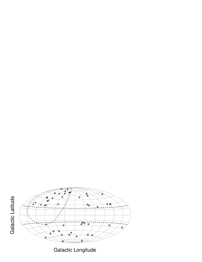
Figure 1: Spatial distribution of our sample. Dashed line represents b=$\pm$20 degree, dotted line represents the selected region of Sample 2 (Grossan). Open circle :  Sample 1(Piccinotti), Cross :  Sample 2(Grossan).

Figures 1 and 2 show the spatial distribution and the relation between X-ray observed luminosity and redshift of all the samples. Putting both samples together, we have analyzed 21 sources of XMM-Newton observation data (13 sources of Sample 1, 8 sources of Sample 2) and 14 sources of ASCA observation data (3 sources of Sample 1, 11 sources of Sample 2). For the other sources, we have used spectral analysis results in literature. Among them, 5 sources were observed with XMM-Newton, 6 with ASCA, and 2 with Beppo-SAX. Thus we get the spectral information on all but one (H 1537+339) AGN in the sample of 49 AGNs defined above. There is no ASCA, XMM-Newton or Beppo-SAX observation data for H 1537+339. Remillard et al. (1993) showed an optical spectrum of the AGN identified with this X-ray source. It had broad-lines and a UV excess, which were typical of a type 1 AGN, and showed no sign of broad absorption lines (BALs). Thus we have assumed that it has an unabsorbed power-law spectrum ($\Gamma=1.8$), which is typical of a type-1 AGN/QSO.

3 DATA REDUCTION AND SPECTRAL ANALYSIS

3.1 Overall Procedure

We have reduced the XMM-Newton data using the Scientific Analysis System (SAS) ver 5.4.1. or later. We have compared the results of the reduction/analysis using SAS ver 6.0 and “Current Calibration Files” (CCF) updated as of December 2004 with those using SAS 5.4.1. for a few selected sources. The change of the results was insignificant for our purposes. About a half of the sources with available XMM-Newton data have such high count rates that CCD pile up affects the spectral analysis. In these cases, we extracted the source spectrum from an annular region with inner and outer radii of about 12$\arcsec$ and 60$\arcsec$ respectively (exact radii vary) to avoid the central peak. A background spectrum was taken from an annular region around the source with the inner radius of 1$\arcmin$, when the observation was made with the full window or large window mode. Small window mode observations are usually made for bright sources and the background are negligible for these observations. Since the XMM-Newton light curve of NGC 5548 had a flare in the last 1/4 of the observation, we did not include this time interval into spectral analysis. In the spectral fitting, we used pulse-height channels corresponding to $0.4-10$ keV and $0.3-10$ keV for MOS and PN detectors respectively.

We have used FTOOLS 5.0 and asca-ANL ver 2.00 to make data reduction and extraction of events for ASCA observation data. The SIS and GIS pulse-height spectra have been created from events screened with the standard screening criteria. Source spectra has been extracted from a 3$\arcmin$ radius circle and background spectra has been accumulated from an off-source area of the same observation for SIS spectra. For the GIS spectra, we have used a 7$\arcmin$ radius region as a source and the backgrounds from 8$\arcmin$ and 11$\arcmin$ annulus region centered on each source of the same observation. The ASCA light curve of MKN 1152 had a flare in the middle and we have excluded the data during the flare. In the spectral fits, we have used pulse-height channels corresponding to $0.7-10$ keV and $1.0-10$ keV for SIS and GIS detectors respectively.

For both XMM-Newton and ASCA data, we have used XSPEC ver 11.0 or later for the spectral analysis. As our first step, we have fitted the reduced pulse-height spectra with a single power-law and intrinsic absorption model (XSPEC model “zwabs”). Galactic absorption (“wabs”) with a fixed column density (Dickey & Lockman 1990) has been always included. This first step analysis have been made in the $2.0-10$ keV range to avoid the effects of soft excess. We have also excluded the $5.5-8.0$ keV range when there was a significant residual caused by absorption edge or 6.4 keV Fe K$\alpha$ line in the spectrum. The second step has been to add additional components, including a soft excess, an absorption edge, a reflection component, or a 6.4 keV Fe K$\alpha$ line to the spectral model and fitted to the full energy range whenever needed to verify that the deviation from the simple best-fit absorbed power-law does not have major effects on the spectral statistic and luminosity function analysis which are made later in this paper. We have also tried to include partial covering and/or ionized absorbers for some sources as described in Sect. 3.2 .

The basic results of the simple absorbed power-law fit parameters (photon index $\Gamma$ and intrinsic neutral absorber’s column density $N_{\rm H}$) are summarized in Tables 3 &  4. These numbers are from our first-step analysis or similar simple absorbed power-law fits from literature except for those detailed in Sect. 3.2.

Piccinotti et al. (1982), used the conversion factor of one R15 count s${}^{-1}\sim 2.17\times 10^{-11}$  erg cm^-2 s^-1 in the $2-10$ keV energy band for a power-law spectrum with photon index 1.65, to derive the flux for most of their AGNs. Since we have spectral information for each object, we have re-calculated the fluxes of Sample 1 objects from the R15 count rate using the actual HEAO-1 A2 response function and our spectral results. The corrected observed flux is listed as the HEAO-1 flux in Tables 3& 4. An underlying assumption is that $\Gamma$, intrinsic $N_{\rm H}$ and other spectral parameters (except the global normalization) of an AGN do not change with the variation of its luminosity. For Sample 2, Grossan (1992) used conversion factor $5.29\times 10^{-9}$  erg cm^-2 s^-1/LASS count s^-1 in the $2-10$ keV energy band appropriate for a power-law spectrum with photon index 1.7 for each flux. We have re-calculated the fluxes using our spectroscopy results for Sample 2 as well.

The luminosities listed in Tables 3 & 4 are intrinsic luminosities, i.e., absorption-corrected luminosity using the fitted N_H. We show the absorption-corrected luminosities because we are more interested in the intrinsic AGN power in the later analysis.

3.2 AGNs with Special Considerations

In this subsection, we summarize the spectral features of the AGNs for which the deviation from the simple power-law absorbed by neutral gas has a major impact on discussing the spectral statistics, intrinsic luminosities, and absorbing column densities. In particular, we have taken special attention to AGNs which gave unusually hard power-law index ($\Gamma\lesssim 1.4$) in the first step simple absorbed power-law fits, since they are likely to be heavily affected by partially covered and/or warm absorbers. Six AGNs in the entire sample have been found to fall in this category as detailed below.

In calculating the intrinsic luminosity, we have used the spectral models involving partial and/or ionized absorbers. The global normalization has been adjusted to give the observed HEAO-1 A2 (A1) count rate, if the AGN belongs to sample 1 or sample 2. The intrinsic luminosity in Tables  3 & 4 have been corrected for all absorbers. For the column density in these tables, we have used the sum of all neutral absorbers (including partial absorbers) as a representative value, but have not included those of any warm (ionized) absorber components. We explain our treatments for these 6 AGNs below.

NGC 7582

A simple absorbed power-law fit to the ASCA data gave $\Gamma=1.2$ and $N_{\rm H}=6\times 10^{22}$  cm^-2. The best description of its X-ray spectrum was given by Turner et al. (2000) from the Beppo-SAX data. Their model included an intrinsic power-law component of $\Gamma=1.95$ absorbed by two components: a totally covering $N_{\rm H,22}=14.4$ absorber and a thicker absorber with $N_{\rm H,22}=160$ blocking $\sim 60\%$ of the X-ray source. We employ this model for de-absorption (see above) and the sum of these two absorbing columns for the representative neutral column density.

3A 0557-383

The hard X-ray source 3A 0557-383 was identified with a Seyfert 1 galaxy. Turner et al. (1996) reported the complex absorption below 2 keV of the X-ray spectrum from an ASCA observation. They found a good fit with either 96 % of the source covered by a column of 3.1 $\times$ 10²²  cm^-2 of low-ionization gas or full covering by a column of 3.6 $\times$ 10²²  cm^-2 of highly ionized gas, and an neutral iron K-shell emission line with equivalent width  300 eV. We used the latter model (Model D of Turner et al. 1996).

Kaz 102

The results of detailed analysis of our own ASCA data of this object have been reported by Miyaji et al. (2003) (M03). Kaz 102 has no sign of heavy absorption or a Fe K$\alpha$ line. A single power-law with $\Gamma\sim 1$ described the ASCA spectrum well, while it had softer spectra when it was observed by ROSAT. This hard spectrum is probably due to extreme warm absorber component and/or reflection as discussed in M03. In this study, we employ the warm absorber model with intrinsic $\Gamma\sim 1.9$ in M03 for absorption correction. No neutral absorber is detected in the analysis and thus we assumed a zero $N_{\rm H}$ for the neutral gas.

3C 445

The nearby broad-line radio galaxy (BLRG) 3C 445 has very hard power law $\Gamma$=1.08 and a large intrinsic absorption ($N_{\rm H}\sim 1.4\times 10^{23}$ cm^-2) in our first-step analysis of the XMM-Newton observation data. In Sambruna et al. (1998), the X-ray spectrum of 3C 445 observed with ASCA were described by a dual absorber with an intrinsic flat power-law ($\Gamma\sim 1.3$) continuum. We have made our own analysis of the XMM-Newton data with two intrinsic absorbers, neutral partial covering and full covering cold gas in $0.6-12$ keV band like Model C of Sambruna et al. (1998). Our analysis show a hard intrinsic power law ($\Gamma$ =1.11$\pm$0.05) absorbed by partial covering ($90\pm 10$%) neutral gas with $N_{\rm H}\sim 1.32\pm 0.06\times 10^{23}$ cm^-2 and no full covering cold gas ($\chi^{2}/d.o.f=1.27/159$).

We employ our XMM-Newton result for intrinsic luminosity calculation and statistics. Taking Sambruna et al. (1998)’s model had negligible effects on the analysis in next sections.

MKN 6

A detailed spectroscopic analysis of this object is given by Immler et al. (2003), who analyzed the same XMM-Newton data combined with Beppo-SAX data. Their joint analysis preferred a model (Model 4) with a fixed-index power law ($\Gamma$=1.81) and two partially covering neutral absorbers (56$\pm$2 % of 8.1$\pm 0.5\times 10^{22}$  cm^-2 and 91$\pm$1 % of 2.3$\pm 0.1\times 10^{22}$  cm^-2), with a very small reflection component. We have re-analyzed the XMM-Newton using this model and checked the spectral fitting results, when $\Gamma$ was set to free parameter. We found a slightly harder spectral index and small column density, but the difference of derived intrinsic X-ray luminosity is less than 10%. This has negligible effects on our HXLF and other statistical conclusions. We listed the sum of column densities of the dual absorbing gas and $\Gamma=$ 1.81 and used the spectral shape of Immler et al. (2003)’s Model 4 for the absorption correction.

NGC 4151

This Seyfert 1.5 galaxy NGC 4151 has long been known that it appears to have a flat power law ($\Gamma$ $\sim 1.3-1.7$), a substantial column density of absorbing gas (N_H $\sim$ 10²³  cm^-2), a strong soft excess at energies below 2 keV, and the broad iron K $\alpha$ emission line. We take the result of Model 2 in Schurch et al. (2003), who modeled the spectrum with two absorption components, a partially photoionized absorber and a neutral absorber, and a neutral reflection continuum. The column density of the neutral absorber is listed in Table 3 and the absorption correction has been made with their Model 2.

3.3 Other Spectral Features

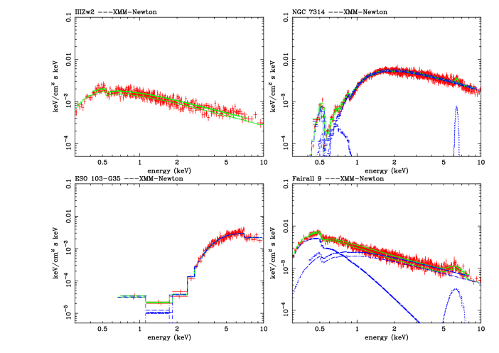
Figure 3: Examples of spectral fit results in the $E\;I(E)$ scale, for IIIZw2, NGC 7314, ESO 103-G35, and Fairall 9 in 0.3-10 keV band. The spectra are represented by thin red crosses, and green and blue lines represent the all model spctrum and each spectral component, respectively. The details of each spectral component are listed in Table 3-6. Figures 3.1 - 3.5 are available in the electronic edition of the Journal.

We have also examined the spectral fits in the broad band spectrum more in detail, in particular, paying attention to the existence of iron lines and/or a soft excess. We have started with a power-law with the photon index fixed to that in first step analysis, with the Galactic absorption at the AGN position. For those where the simple absorbed power-law model have significant residuals in the broad-band spectrum, we considered more complicated models, involving, e.g., a soft excess and or an iron line. The fitting results with the soft excess are shown in Table 5. We listed the only best fit results for soft excess, within several spectral model fittings (blackbody, broken-power-law, 2-powerlaw, soft thermal emission, dual absorber, etc.. ). Typical spectrum of the sample in our spectral fitting are shown in Figure 3. For those the addition of an iron line improved the fit, the central energy, normalization, and equivalent width the line, represented by a single Gaussian, are listed in Table 6. In the spectrum of MKN464, there are significant residuals in $1.5-3.0$ keV band and this range has been excluded for the analysis.

The photon index and intrinsic column density for most of all AGNs are consistent to that in first step analysis within errors, even if the photon index and the intrinsic absorption ($N_{\rm H}$ in “zwabs”) are set to free parameters in this second-step spectral analysis. Thus the existence of soft excess and iron emission line does not have significant effect in our further analysis.

The statistics of such features has its own importance. However, in our current data, the limits on the detection of these features vary observation by observation and difficult to model. Thus one should not take advantage of the good completeness of our sample to make a statements on the statistical properties of the iron lines and soft excess in combination with our sample definition.

4 STATISTICS OF SPECTRAL PROPERTIES

4.1 Neutral $N_{\rm H}$ and Photon Index Distribution

Figure 4 shows the distribution of the absorbing column densities (N_H) of neutral absorbing gas intrinsic to the AGNs. As described in Sect. 3.2, we have added the value of any partial covering neutral column densities to the $N_{\rm H}$ value used here. On the other hand, the column densities of ionized absorbing gas have not been included (3A 0557, Kaz 102, NGC 4151). This is because the neutral gas and ionized gas come from different regions, the former being in a molecular torus at about $10^{18}-10^{20}$ cm from the nucleus, while the latter at a region closer to the nucleus ($\sim 10^{17}$ cm, (e.g. Reynolds & Fabian (1995)). Thus they do not have much relevance to each other.

We also plot an expected relative spatial number density in each $N_{\rm H}$ bin, assuming a Eucleadian $\log\,N-\log\,S$ relation for the intrinsic flux distribution of the X-ray AGNs:

$$N_{\rm spatial}=\left(\frac{f_{\rm intrinsic}}{f_{\rm absorbed}}\right)^{1.5}\times N_{\rm raw}$$ (1)

in which, $N_{\rm spatial}$ is spatial number density, $f_{\rm intrinsic}$ is intrinsic flux of primary X-ray component, $f_{\rm absorbed}$ is observed flux (after absorption), and $N_{\rm raw}$ is the raw number in the $N_{\rm H}$ histogram. Upon calculating the $f_{\rm intrinsic}$ of each bin, we have assumed that the intrinsic power-law source of $\Gamma=1.7$ was absorbed by cold gas of mean column density of each bin. This may not be correct in case of the source has partially covering absorbers. However, the effect is much smaller than the errors due to small number statistics in each bin.

Figure 5 shows the distribution of spectral photon index. The $\Gamma$ values of NGC 3227, 3A 0557, Kaz 102, H 1537+339, and MKN 6 are excluded from the histogram, because they have been fixed during the spectral fit, or no detailed spectral information. The mean photon index is 1.76 with $\sigma=0.2$. This is similar to the result of Williams et al. (1992), who studied an incomplete sample of 13 QSOs observed by GINGA and obtained the result of the mean photon index of 1.81$\pm$0.31. Even if we use the results from first-step single absorbed power-law fit results (Sect. 3) the 6 sources discussed in Sect. 3.2, the mean photon index has not change remarkably, giving 1.72$\pm$0.24. In George et al. (2000), the mean photon index has $\sim 2.0$ for various spectral analysis, while the relatively wider distribution ($1.3<\Gamma<3.0$). And in Reeves & Turner (2000), they derived mean photon index $1.89\pm 0.05$ with $\sigma=0.27$. The two other observations are somewhat softer distributions, which is assumed be due to the effect of a reflection component. We have found no correlation between $\Gamma$ and hard X-ray luminosity, which is consistent with results of George et al. (2000), and Reeves & Turner (2000).

4.2 Relation between Hard X-ray Intrinsic Luminosity and $N_{\rm H}$

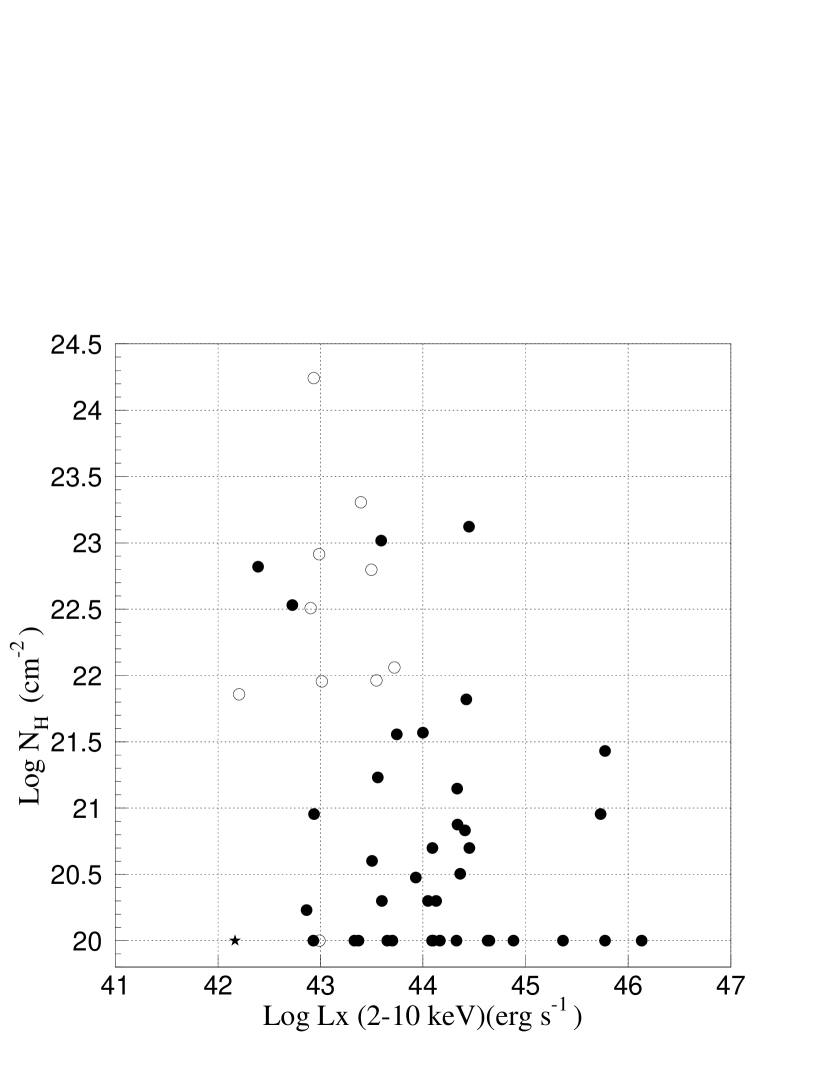
Figure 6: Relation between hard X-ray luminosity and intrinsic N_H. Type 1 galaxy (Seyfert 1, 1.5, Type 1 QSOs) are shown as filled circles and Type 2 AGNs (Seyfert 1.9 - 2) are shown as open circles respectively. One probable LINER is plotted with a filled star. The luminosity is intrinsic (before absorption).

Figure 6 shows the scatter of the AGNs, in the hard X-ray luminosity – intrinsic neutral $N_{\rm H}$ plane. Different symbols are used for AGNs with different optical types, i.e. type 1 (Seyfert 1-1.5, type1 QSO, or BLRG), type 2 (Seyfert types above 1.8) AGNs or LINER candidate. Most of optical type 1 AGNs have small X-ray absorption, $\log\,N_{\rm H}\leq$ 21.5, and most of Seyfert 2 galaxies have large X-ray absorption, $\log\,N_{\rm H}\geq$ 21.5 as widely known. Some AGNs optically classified as type 1 have large $N_{\rm H}$ ($\log\,N_{\rm H}\gtrsim$ 21.5) values. They usually have X-ray spectra involving partially covering absorbers. We have include such sources in the absorbed AGN group for the HXLF analysis. The optical classifications in this paper are not necessarily accurate, because they are based on the detection significance of broad emission lines and depend on the quality of the optical spectra. Indeed, there are some AGNs (ESO103-G35, NGC526a, 3c445, etc..) for which different sources give different optical classifications. However, our spectral results may suggest that the anomalous cases reflect the existence of substantial variance in the dust to gas ratio, or a geometrical separation to the line of sight. More significant data analysis with careful regard to the variability would derived whether these objects are common in AGNs or not.

We observe no AGN with $\log\,L_{\rm x}>44.5$ and $\log\,N_{\rm H}\gtrsim$ 21.5. This is consistent with U03’s analysis including ASCA and Chandra surveys, which find a decrease of absorbed AGN fraction towards high intrinsic luminosities. A further discussion of this effect will be given in Sect. 6.

5 LOCAL HARD X-RAY LUMINOSITY FUNCTIONS

Our purpose of this section is to calculate the local Hard ($2-10$ keV) X-ray Luminosity Function (HXLF) of AGNs from our sample. We have taken the U03’s approach and constructed the $2-10$ keV HXLFs for the intrinsic X-ray luminosity. We have divided the sample into unabsorbed and absorbed AGNs at $\log\,N_{\rm H}=21.5$ for the use with HXLF analysis. The number of X-ray absorbed AGNs is 16, while that of X-ray unabsorbed AGNs is 33 in our sample.

We have used the $\Sigma V_{\rm a}^{-1}$ estimator (Avni & Bahcall 1980), which is a modified version of original $\Sigma V_{\rm max}^{-1}$ (Schmidt 1968). We can write the binned HXLF as,

$$\frac{d\Phi}{d\log\,L_{\rm x}}(\log\,L_{\rm x})\approx\Sigma_{i}\frac{1/V^{i}_{\rm a}}{(\Delta\log\,L_{\rm x})}$$ (2)

where $V^{i}_{\rm a}$ is the available comoving volume in which the $i$-th AGN would be in the sample, within the redshift range. The $V^{i}_{\rm a}$ value can be expressed by

$$V^{i}_{\rm a}=\int^{z_{\rm max}}_{z_{\rm min}}d_{\rm A}(z)^{2}c\frac{d\tau}{dz}(z)\cdot A_{\rm eff}({\rm CR})~{}{\rm d}z$$ (3)

where $d_{\rm A}(z)$ is the angular distance, $d\tau/dz(z)$ is the differential look back time per unit z, CR is the observed count rate of the AGN if it was placed at the redshift $z$, and $A_{\rm eff}({\rm CR})$ is the survey area as a function of the count rate. We take $z_{\rm min}$ = 0 and $z_{\rm max}$ = 0.4 to include all the AGNs in the sample.

Since our sample consists of two subsamples defined in the count rate limits from two different detectors, our $V_{\rm a}$ consists of two parts:

$$V^{i}_{\rm a}=V^{i}_{\rm a,1}+V^{i}_{\rm a,2},$$ (4)

where $V^{i}_{\rm a,1}$ and $V^{i}_{\rm a,2}$ are the comoving volumes of the universe within which the $i$-th AGN would be observable in the Sample 1 and Sample 2 respectively. In calculating $V^{i}_{\rm a,2}$ of an AGN in Sample 1, we have used the predicted LASS  cts s^-1 cm^-2 of HEAO-1 A1 experiment, which has been estimated by using the HEAO-1 A2 R15CR, the spectral shape of this source, and the detector responses of HEAO-1 A2 experiment, and vice versa. In the HXLF calculation, we have used the observed flux (i.e. after absorption) in estimating the $V^{i}_{\rm a}$, while X-ray intrinsic luminosity (de-absorbed luminosity) has been used to divide the sources into luminosity bins.

As mentioned in Sect. 2, we have used the effective survey area for Sample 2 after correcting the LASS count rate for the effects of confusion noise. This correction is discussed in detail in Appendix A. After the correction, the area as a function of the corrected count rate gradually decreases as the $CR_{\rm corr}$ decreases to the limit of 1.9 $\times 10^{-3}$ LASS cts s^-1 cm^-2.

A small number of very luminous AGNs in our sample are observable at redshifts where evolution has a non-negligible effect ($z\gtrsim 0.2-0.3$). Thus we have also derived the evolution-corrected HXLF by giving weights to the $V^{i}_{\rm a}$ calculation,

$$V^{i\prime}_{\rm a}=\int^{z_{\rm max}}_{z_{\rm min}}d_{\rm A}(z)^{2}c\frac{d\tau}{dz}(z)\cdot A_{\rm eff}(CR)(\frac{1+z}{1+z_{0}})^{p}~{}{\rm d}z,$$ (5)

with which we can estimated the HXLF at $z=z_{0}$ by including the density evolution factor $[(1+z)/(1+z_{0})]^{p}$. We use the index $p=5$, which is consistent with the soft X-ray luminosity function evolution by Hasinger et al. (2005). The impact of the evolution to the XLF was found to be as small as $\sim 10\%$ in the $45.5<\log\,L_{\rm x}<46.5$ bin. Since our sample is mainly local, K-correction has a negligible effect. Most luminous AGNs are unasborbed with the photon index $\sim$ 1.9, with very little K-correction even at $z=0.4$. Absorbed AGNs typically have such low luminosities that they are not detectable at high enough redshifts for the K-correction to be important. The K-corrections are typically $\lesssim$ 5% for the absorbed AGNs.

Figure 7 shows the Hard X-ray luminosity function calculated from our sample for the evolution-corrected case. We take $z_{0}=0$ for Figure 7. We have made the luminosity bins same in all HXLF calculations for comparisons. We only have upper limits for absorbed AGNs in the three highest luminosity bins and we plot only interesting (90%) upper limits, i.e. those which make significant constraints. Figure 7 clearly shows different X-ray luminosity function slopes between absorbed and uabsorbed AGNs at the high luminosity end. The ratio of absorbed / unabsorbed XLF is 2.35$\pm$2.1 in $\log\,L_{\rm x}\sim 42-44$, and 0.11$\pm$0.08 in $44-44.5$). The significance of the difference of the absorbed/unabsorbed ratio in these two luminosity bins has been estimated using a bootstrap resampling. Out of all the 41 AGNs in the $\log\,L_{\rm x}\sim 42-44.5$ range, we have randomly resampled the same number of AGNs allowing duplicates. The ratio of the absorbed / unabsorbed HXLFs in the two luminosity ranges have been calculated for each of 10000 bootstrap-resampled samples. As a result, the probability that the ratio reverses, i.e., absorbed / unabsorbed ratio becomes greater in the higher luminosity bin, turns out to be only less than 0.4%.

In order to compare absorbed and unabsorbed AGN HXLFs more quantitatively, we also made a maximum likelihood (ML) technique. The ML-fitting of the HXLF to the data where individual AGNs have different spectra is not straightforward. We use U03’s approach in fitting $N_{\rm H}$ function and the intrinsic HXLF. There is a limitation in this approach, however, that we have to assume a simple absorbed power-law spectrum for each source. For the fits, we have used the sources in the range $z<0.2$ and $\log\,N_{\rm H}<24$ to compare with the U03 results. We again divided into unabsorbed and absorbed AGNs at $\log\,N_{\rm H}=21.5$ in this sample. In this analysis, the $N_{\rm H}$ function was assumed to be constant within each of $\log\,N_{\rm H}<21.5$ and $21.5<\log\,N_{\rm H}<24$ bins. The fits do not depend significantly on details of the evolution within the small redshift range. Thus, a pure density evolution model by U03 ($e(z)=(1+z)^{4.2}$) was used to represent the small amount of evolution. The best-fit parameters of the XLFs were calculated following the same procedure as U03.

Table 7 shows the best fit parameters from the ML-fits. The fit result from U03’s PDE model is also listed. The two power-law indices for the ’All’ sample are consistent with that in U03, while the normalization $A$ seems larger than the U03 value. This is partially because $A$ is strongly depend on the $\log\,L_{*}$, parameter, for which we found a somewhat smaller value. Also, U03 is based on the global fit to all redshifts, where the higher redshift samples contribute much of the constraints to the relevant parameters. In comparing absorbed and unabsorbed AGN samples, the ML fits have been made with a fixed $\log\,L_{*}=44.0$ in order to avoid strong dependence between fitting parameters. This value is consistent with the best-fit values for both samples, when fitted with this parameter free. As expected, the $\gamma_{2}$ of absorbed sample is significantly steeper than that of unabsorbed AGNs.

In Fig. 7 (evolution-corrected to $z=0.1$), we overplot the best-fit result of smoothed two power law formula for SXLF in the $0<z<0.2$ bin by Hasinger et al. (2005). The $0.5-2$ keV SXLF has been converted to $2-10$ keV band using a $\Gamma=1.8$ power-law spectrum. Our evolution corrected HXLF of unabsorbed AGNs obtained from our sample is marginally consistent with the Hasinger et al. (2005) best-fit model. We also overplot the results from Sazonov (2004) for unasborbed and total AGNs. They used the $3-20$ keV band, where the attenuation of flux by absorption have only minor effect (by $\sim$ 8% for $\log\,N_{\rm H}=$22.5). We have thus converted their $3-20$ keV HXLFs (for luminosities uncorrected for absorption) to $2-10$ keV using a $\Gamma=1.8$ power-law for overplots. Detailed comparisons are discussed in Sect. 6.

6 DISCUSSION

6.1 Comparisons of Luminosity Functions and Volume Emissivity

We have calculated the local HXLF with binned $\Sigma V_{\rm a}^{-1}$ method for our sample defined with HEAO-1 experiment. The HXLF for our $\log\,N_{\rm H}<21.5$ results is marginally consistent with the best-fit model of SXLF in the $0<z<0.2$ bin in Hasinger et al. (2005) as well as with the results from Sazonov (2004) for unasborbed and total AGNs. It is not surprising that we have small discrepancies because our $\log\,N_{\rm H}<$ 21.5 selection does not necessarily match with Hasinger’s soft X-ray type 1 selection. A notable exception is the $44<\log\,L_{\rm x}<44.5$ bin, where our sample gives an excess which cannot be explained by statistics alone.

The local X-ray volume emissivity of brightest AGNs can be estimated by $\Sigma_{i}(L_{\rm x,i}/V^{i}_{\rm a})$. The volume emissivity value estimated from our sample is $\rho_{2-10~{}{\rm keV}}=5.85\pm 1.17\times 10^{38}$ erg s^-1 Mpc^-3, which is derived using observed luminosity (absorbed). Note that there is no AGN with $\log\,L_{\rm x}<42$ erg s^-1 in our sample.

Miyaji et al. (1994) estimated the $2-10$ keV local volume emissivity by modeling the cross-correlation between the all-sky cosmic X-ray background (CXRB) surface brightness from the HEAO-1 A-2 experiment and the IRAS galaxies, obtaining ($6.1\pm 1.7)\times 10^{38}$  erg s^-1 Mpc^-3 (for $H_{0}=$ 70 km s^-1 Mpc^-1). This is consistent with the AGN volume emissivity from our sample, implying that the contribution of lower luminosity sources (e.g., star-forming galaxies and LINERS) as well as other sources, non-active galaxies to the local volume emissivity is very small. On the other hand, Sazonov (2004) estimated the X-ray ($3-20$ keV) volume emissivity of $\log\,L_{\rm x}>$ 41 erg s^-1 from emission line AGNs with RXTE All Sky Slew Survey and found $\rho_{3-20~{}{\rm keV}}$($>~{}41$) = ($4.9\pm 1.2)\times 10^{38}$ erg s^-1 Mpc^-3, (for $H_{0}=$ 70 km s^-1 Mpc^-1, $z>$ 0.001), which can be converted to ($2.7\pm 0.7)\times 10^{38}$ erg s^-1 Mpc^-3 in the $2-10$ keV band using the absorbed power-law model of AGNs estimated based on the RXTE hardness ratios. Their local volume emissivity estimate is only about a half of our current estimate. One possibility is an effect of local large-scale structure at $z<0.015$, where our sample and the RXTE sample have different weights.

The HXLF from our sample seems larger than that of RXTE with $\log\,L_{\rm x}\sim 44-44.5$. There is a possibility of some systematic in Sazonov (2004)’s $2-30$ keV to $2-10$ keV conversion. Their absorbed $\Gamma=1.8$ power-law model fit to the RXTE hardness ratio based on $3-8$ and $8-20$ keV count rates is only sensitive to $\log\,N_{\rm H}>$ 22. Also their harder band is likely to be affected by reflection bumps. At this moment, we are not certain whether the differences in the volume emissivity and HXLF results are due to the large-scale structure (cosmic variance) effect, assumed spectra in band conversions, or other systematics. A similar study with a large-scale sensitive hard X-ray survey with sufficient AGNs to exclude the $z<0.015$ universe and to sample a large volume of the present-day universe, such as available from eROSITA or MAXI will give an ultimate solution.

6.2 Luminosity – Absorbed AGN fraction Relation

One way of testing the simplest unified scheme, where the difference between absorbed and unabsorbed AGNs are purely from the orientation effect and the intrinsic properties are essentially the same is to compare the shapes of unabsorbed and absorbed AGN XLFs in intrinsic (i.e. de-absorbed) luminosity. We have found a difference between the HXLFs of the X-ray absorbed AGNs and that of unabsorbed AGNs in that the number density of absorbed AGNs drops more rapidly than unasborbed ones towards high luminosities. This trend can be also seen in the scatter of the sample AGNs in the hard X-ray intrinsic luminosity versus intrinsic neutral $N_{\rm H}$ diagram in Figure 6, in which we see a void of AGN in $\log\,L_{\rm x}>44.5$, $\log\,N_{\rm H}>$ 21.5. This trend has been clearly demonstrated by U03 as the decreasing absorbed fraction of AGNs as a function of intrinsic luminosity from a larger sample including AGNs in this work, from ASCA and from Chandra surveys. This lead U03 to suggest a modified AGN unified scheme, where the difference between type 1 (unabsorbed) and type 2 (absorbed) AGNs is not solely due to the viewing angle effect, but involves some intrinsic difference of the geometric and/or physical conditions of the absorbing tori around the SMBH based on the radiative power of the primary X-ray component.

To verify that the high-luminosity high-absorption void really reflects the actual deficiency of high-luminosity highly absorbed AGNs rather than by a selection effect in our sample, we calculate the expected number of AGNs in the case where the simplest unified scheme was true, i.e., there was no intrinsic difference in the absorbing geometry as a function of AGN power. We have started with the smoothed two-power-law expression of the $0.5-2$ keV soft X-ray luminosity function in the $0.015<z<0.2$ bin by Hasinger et al. (2005). We have slightly tweaked the parameters and added AGNs in the absorbing columns of $\log\,N_{\rm H}$=20, 21., 22, 23, and 24 with the same luminosity function shape, allowing the relative normalization to vary, following an approach similar to an AGN population synthesis model. The ratios of number densities in each $N_{\rm H}$ bin have been adjusted to match the actual numbers of AGNs in $\log\,N_{\rm H}$ ranges of $<20.5$, $20.5-21.5$, $21.5-22.5$, $22.5-23.5$, $23.5-24.5$ respectively. A further tweak of the parameters have also made to reproduce the number of AGNs in $\log\,N_{\rm H}<$ 21.5, $\log\,L_{\rm x}>44.5$ region (luminous unasborbed AGNs). An important assumption in this model is that the shape (all parameters besides normalization) are identical for all $N_{\rm H}$ classes. The expected number of AGNs in the “luminous absorbed” void under this model turns out to be five, while we observe none. Four of the five AGNs expected under this model would be in Sample 1, where only one of 57 X-ray sources are unidentified. Treister et al. (2005) suggested that apparent such effect could arise from selection effects, their analysis is based on a Chandra survey focusing on a much fainter population with limited identification completeness. Their argument does not apply to our analysis or that of U03, involving highly complete samples. (See also Treister & Urry (2005), where they also found this effect by including more samples.)

Recently Zhang (2005) made an interesting suggestion that, if most of the intrinsic power-law component in the X-ray spectra of AGNs is from a Comptonized emission by optically thick hot plasma above the accretion disk, this relation can be explained solely by the viewing angle effect due to geometrical projection. This assumption needs a physical condition that the planes of the accretion disk and the dusty torus are co-aligned. We note also that the Comptonizing plasma need to have a planer geometry and to be parallel to the accretion disk. If the emission region is optically thin and/or composed of hot spots rather than a planer region, the projection effect would not arise.

6.3 Flux Variability

In our investigation, a complete flux-limited sample of brightest objects were re-observed with XMM-Newton, ASCA and/or Beppo-SAX. We plotted the re-observed flux versus HEAO-1 observed flux in Fig. 8 for unabsorbed and absorbed AGNs. The HEAO-1 flux has been corrected for the confusion noise bias described in Appendix A. We see from Fig. 8 that most AGNs show lower fluxes upon the re-observations, even after the correction.

The decrease can be naturally explained as a result of AGN variability and the $\log\,N-\log\,S$ distribution of the AGNs which rises rapidly as flux becomes lower. A flux-limited brightest sample is more likely to pick up an AGN’s brighter than average state, while the re-observation picks up all states equally. We formulate this effect as follows.

At sufficiently bright fluxes, the $\log\,N-\log\,S$ relation follows the Euclidean relation

$$N(>S)\propto S^{-1.5},$$ (6)

or in the differential form

$$n(S)=dN(S)/dS\propto S^{-2.5}$$ (7)

For the convenience of the calculations, we define $l\equiv\ln\,S$. Then, Eq. 7 can be rewritten as:

$$n(l)dl\propto e^{-1.5l}dl$$ (8)

Suppose that the variability of each individual AGN is characterized by the Gaussian log-flux distribution with a standard deviation $\sigma$:

$$v(l^{\prime},l)=(2\pi\sigma^{2})^{-1/2}\exp[-(l-l^{\prime})^{2}/(2\sigma^{2})],$$ (9)

the apparent source count above a log flux of $l_{0}$ at the time of the survey observation can be expressed by

$$N^{\rm obs}(>l_{0})=\int^{\infty}_{-\infty}\big{\{}n(l^{\prime})\int^{\infty}_{l_{0}}v(l^{\prime},l)dl\big{\}}dl^{\prime},$$ (10)

If an AGN whose average log flux is $l^{\prime}$ was observed at $l$ at the time of the survey, the expectation value of its flux upon the re-observation is $l^{\prime}$. Therefore the expectation value of the decrease of the flux ($\langle dl\rangle\equiv\langle l^{\prime}-l\rangle$) can be expressed by

$$\langle dl\rangle=\frac{\int^{\infty}_{-\infty}\big{\{}n(l^{\prime})\int^{\infty}_{l_{0}}v(l^{\prime}:l)(l-l^{\prime})dl\big{\}}dl^{\prime}}{\int^{\infty}_{-\infty}\big{\{}n(l^{\prime})\int^{\infty}_{l_{0}}v(l^{\prime}:l)dl\big{\}}dl^{\prime}}$$ (11)

Under the assumption that $n(l^{\prime})$ follows the Eucleadean relation Eq. 8 and log normal flux distribution of AGN flux variation in Eq. 9, and by further assuming that all AGNs vary at a typical amplitude characterized by $\sigma$, Eq. 11 can be integrated numerically. Figure 9 shows the numerical solution of Eq. 11 in the $\sigma-\langle dl\rangle$ plane. ¿From Fig. 9, we see that $\langle l\rangle$ is always positive, which means re-observation give lower fluxes on average. This is partially because there are much more fainter AGNs under the distribution Eq. 7. Thus the net effect of AGN variability is that AGN in the flux-limited sample seems to show a flux decrease upon the re-observation on average. In turn, from the average decrease of the flux, we can estimate the typical AGN variability amplitude. In our sample, the re-observed flux by ASCA, XMM-Newton or Beppo-SAX was smaller than the HEAO-1 flux by a factor of 0.28 on average (after correction for spectral response and confusion). Figure 9 shows that this corresponds to $\sigma=$ 0.914 or a typical variability amplitude of a factor of 2.5.

7 CONCLUSIONS AND PROSPECTS

We summarize our investigation and main conclusions below.

1. We have defined a complete flux-limited sample from a combination of HEAO-1 A2 and A1/A3 surveys with a well-defined flux-survey area relation. The sample is composed of 28 AGNs from Piccinotti et al. (1982) and 21 AGNs from a deeper sample by Grossan (1992).

2. A bias to the measured flux due to confusion noise have been found to be significant in Sample 2 (A1/A3). We have modeled and made first-order corrections to the fluxes and survey areas.

3. We have obtained X-ray spectral information for all (but one) AGNs in the combined sample from XMM-Newton, ASCA and Beppo-SAX.

4. The spectra have been first modeled as an absorbed power-law. We have made closer look at 6 AGNs which gave spectral index of $\Gamma<1.4$ in this fit and used models involving (multiple) partial covering and/or ionized absorbers.

5. We have found the mean photon spectral index of $\Gamma\approx 1.76$ with a 1$\sigma$ dispersion of 0.2.

6. We find the $N_{\rm H}$ distribution for our sample, which can be used as a constraint to X-ray population synthesis modeling.

7. We have constructed local hard X-ray luminosity functions (HXLFs) from our sample, separately for absorbed and unabsorbed AGNs, as well as for both, as a function of the intrinsic $2-10$ keV luminosity. We have also made HXLFs which have been corrected for density evolution.

8. The scatter of the sample AGNs in the $N_{\rm H}$ versus intrinsic luminosity plane shows a void of AGNs at a high-luminosity, high absorption regime, where we expect $\sim 5$ AGNs if the intrinsic luminosity functions between absorbed and unabsorbed AGNs were identical. This, as well as the difference in the HXLFs between absorbed and unabsorbed AGNs, is not likely due to selection effects.

9. The X-ray fluxes of AGNs in the sample observed by XMM-Newton, ASCA and/or Beppo-SAX were on average lower than those observed by HEAO-1 for the same objects. The mean flux decrease upon re-observation of AGNs in a flux-limited sample has been formulated can be naturally explained by the AGN variability, where the AGNs are likely to have brighter-than-average flux at the time of the sample-defining survey.

As a concluding remark, we note that the sensitivity of large-area surveys at hard X-ray bands currently available is still not sufficient, in contrast with the soft band, where ROSAT All-Sky Survey produced enormous dataset to sample the present-day universe unabsorbed AGN population. In this work, we had to depend on data obtained in the 1970’s to define our sample, to include the absorbed AGN population. Because of this, our investigation is subject to fundamental limitations in terms of object count statistics, confusion and mis-identification problems. To obtain sufficient number of AGNs, we also had to use very nearby objects ($z<0.015$), where the quantities such as HXLF or volume emissivity is subject to the density fluctuations due to the local large scale structure. The understanding of AGN evolution is never complete until we sample the present-day universe fairly. In the near future, a slew survey from the Swift BAT mission (Markwardt et al. 2005) and a dedicated all-sky exposure with INTEGRAL will produced a less biased bright end catalog of AGNs and after a spectroscopic followup such as this work, we expect improvements in our knowledge in this region. Future missions such as MAXI, and eROSITA would find numerous AGNs in our local universe will enable us to make a precision statistics of AGNs in the present-day universe.

Appendix A Correcting for Confusion Effects on HEAO-1 A1 Counts

Our sample selections are partially based on count rates (CRs) observed by the HEAO-1 A1 experiment, which have been cataloged by Wood et al. (1984) (hereafter W84). The CR limit imposed by Grossan (1992) of $CR_{\rm lim}=3.6\times 10^{-3}$ LASS cts s^-1 cm^-2 is subject to confusion noise, in addition to the formal error given by W84, which only includes the effects of photon counting statistics. Due to these effects, the CRs are subject to systematic overestimations near the detection limit. This may bias the estimates of luminosity function derived in Sect. 7.

We have made a first-order correction to these effects by Monte-Carlo simulations. We have taken the following steps.

1. Sources are generated based on approximate $\log N-\log S$ relation, extrapolated down to approximately one order of magnitude below our flux limit. In this simulation, LASS CRs ($CR_{\rm A1}$) have been used rather than fluxes in physical units, because we define our limit by CRs. From the W84 catalog, we have estimated:

   $$N(>CR_{\rm A1})=7\times 10^{-3}(CR_{\rm A1}/5\times 10^{-3})^{-1.5}[{\rm deg}^{-2}]$$ (A1)

2. For each generated source with true underlying CR ($CR_{\rm gen}$), an observed CR ($CR_{\rm obs}$) has been simulated by

   $$CR_{\rm obs}=CR_{\rm gen}+\Delta CR_{\rm err}+\Delta CR_{\rm cfs},$$ (A2)

   where $\Delta CR_{\rm err}$ simulates the deviation due to photon counting statistics and $\Delta CR_{\rm cfs}$ due to confusion noise as detailed below.

   • For a given $CR_{\rm gen}$, an error $\sigma$ is selected from objects in $|b|>30$, $|EB|>35$, and $CR<0.01$, where EB is the ecliptic latitude. $\Delta CR_{\rm err}$ is derived from a random Gaussian deviation using the selected $\sigma$. This may underestimate errors for brighter sources, but the effects we consider is only non-negligible for sources near detection limits.

   • $\Delta CR_{\rm cfs}$ is derived from Monte-Carlo simulations, where objects are generated based on Eq. A1 in the range $5\times 10^{-5}<CR<3.6\times 10^{-3}$ (the upper bound is our flux limit) and distributed over the HEAO-1 A1 beam (W84). The total CRs folded with the beam ($CR_{\rm beam}$) have been calculated for 2000 runs. If $CR_{\rm beam}$ is greater than 3.6$\times$10^-3 above the mean value, the run is rejected.

   • The mean value ($\langle CR_{\rm beam}\rangle$) has been recalculated after the rejection. Then $\Delta CR_{\rm cfs}$ has been calculated as $CR_{\rm beam}-\langle CR_{\rm beam}\rangle$, where $CR_{\rm beam}$ is taken from one of the simulation runs which was not rejected.

3. In order to simulate detected sources, only those with $CR_{\rm obs}>3.6\times 10^{-3}$ have been selected ($CR_{\rm obs}$ of the selected objects is indicated by $CR_{\rm det}$, representing ’detected count rates’). Figure 10(a) shows the scatter diagram of $CR_{\rm det}$ versus $CR_{\rm gen}$ for those objects. The simulated objects have been then binned by $CR_{\rm det}$ and the mean value of $CR_{\rm gen}$ ($\langle CR_{\rm gen}\rangle$) has been calculated in each bin. This gives a measure of mean expected true CR of the sources as a function of the detected CR.

4. Our next step is to find a smooth analytical representation of $\langle CR_{\rm gen}\rangle/CR_{\rm det}$ as a function of $CR_{\rm obs}$. Since we know that $\langle CR_{\rm gen}\rangle/CR_{\rm det}$ goes asymptotically close to unity at higher count rates, we have used the form:

   $$C_{\rm cr}\equiv\langle CR_{\rm det}\rangle/CR_{\rm det} =1-\exp[-(CR_{\rm det}-s_{\rm cr})/w_{\rm cr})],$$ (A3)

   $$(CR_{\rm det}\geq CR)$$

   where $C_{\rm cr}$ represents the CR correction factor. By a $\chi^{2}$ fit with the standard deviation of $CR_{\rm gen}$ in individual bins as $\sigma$, we find the best-fit values:

   $$s_{\rm cr}=1.6\times 10^{-3};w_{\rm cr}=2.6\times 10^{-3}.$$ (A4)

   The binned $\langle CR_{\rm gen}\rangle/CR_{\rm det}$ values are plotted against $CR_{\rm det}$ in Fig. 10(b) along with the best-fit function form. Note that we use $\chi^{2}$ with these $\sigma$’s only as a weighting scheme for the fit and the formal parameter errors of the $\chi^{2}$ statistics does not have any meaning.

5. The detected CRs have been corrected by $CR_{\rm corr}=C_{\rm cr}~{}CR_{\rm det}$. By this correction, the estimated ’true’ count rate for a source detected at the faintest limit of $CR_{\rm det}=CR_{\rm lim}=3.6\times 10^{-3}$ becomes $CR_{\rm corr,lim}=1.9\times 10^{-3}$.

6. In calculating the XLF, we also have to correct the survey area for incompleteness of the detection, where not all sources with a true count rate of, e.g. $>1.9\times 10^{-3}$ will have $CR_{\rm obs}>3.6\times 10^{-3}$. This is made by dividing the differential $\log N-\log S$ curves of $CR_{\rm corr}$ by that of $CR_{\rm gen}$ calculated using the simple geometrical area ($A_{\rm geo}$) of the survey. Using the same functional form as Eq. A3, the effective survey area as a function of $CR_{\rm corr}$ is expressed by

   $$A_{\rm eff}/A_{\rm geo} =1-\exp[-(CR_{\rm corr}-s_{\rm A})/w_{\rm A}], (CR_{\rm corr}\geq CR_{\rm corr,lim})$$ (A5)

   $$=0, (CR_{\rm corr}<CR_{\rm corr,lim}).$$

   We have found the best-fit values of the parameters:

   $$s_{\rm A}=-3.3\times 10^{-3};w_{\rm A}=8.5\times 10^{-3}.$$ (A6)

   The resulting effective area curve is plotted against $CR_{\rm corr}$ in Fig 10(c).

7. Using the corrected $CR_{\rm corr}$ and $A_{\rm eff}$, a corrected $\log N-\log S$ curve has been calculated to see that it is in reasonable agreement with the initially assumed one. This curve is plotted in Fig 10(c) along with those from $CR_{\rm det}$ and $CR_{\rm corr}$ using the geometrical area.

8. Now we are ready to calculate the luminosity function from the real data by applying the corrections Eqs. A3 & A5. to the cataloged CR and geometrical area respectively.

We have also made the same experiment for Sample 1 based on the HEAO-1 A2 Piccinotti et al. (1982) catalog. The effects are negligible in the case of Sample 1.

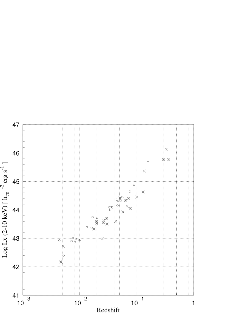
Figure 2: Relation between X-ray luminosity and redshift of the sample. Open circle : Sample 1 (Piccinotti). Cross : Sample 2 (Grossan). For Sample 2, the flux is calculated from the corrected count rate described in Appendix A.

Figure 4: The intrinsic N_H (neutral) distribution of the AGNs in our sample. We also plotted spatial number density calculated from Eq. 1.

Figure 5: Photon index distribution of the sample. The open histogram represents all the sample, the filled histogram represents X-ray absorbed AGNs.

Figure 7: Hard X-ray luminosity functions for all AGNs (black, square), X-ray unabsorbed AGNs (red, circle), and absorbed AGNs (blue, triangle) in our sample for the evolution-corrected case. Thick solid lines and dotted lines show the ML-fitting results of the XLFs for unabsorbed and absorbed AGNs, respectively. Thin solid lines show type 1 AGN XLF from Hasinger et al. (2005). Thin dashed and dotted lines show the results from Sazonov (2004) for all AGNs and unabsorbed AGNs respectively. All overplotted lines have been converted to 2-10 keV from the originals assuming a $\Gamma=1.8$ power-law. Errors are 1$\sigma$.

Figure 8: Relation between ASCA or XMM-Newton observation flux and HEAO-1 observation flux. Circle : unabsorbed AGNs. Triangle : absorbed AGNs.

Figure 9: The numerical solution of Eq. 11 in the $\sigma-\langle dl\rangle$ plane, where $\sigma$ is typical deviation of the variability of AGN flux, and $\langle dl\rangle\equiv\langle l^{\prime}-l\rangle$ represents the expectation value of the decrease of the flux. We can estimate a typical $\sigma$ of our sample from this $\sigma$ - $\langle dl\rangle$ relation under the assumption discussed in Sect. 6.3.

Figure 10: (a) The scatter diagram of the generated “true” count rate ($CR_{\rm gen}$) versus the detected count rate ($CR_{\rm det}$) in our simulation. The solid line shows $CR_{\rm gen}=CR_{\rm det}$. (b) The $\langle CR_{\rm gen}\rangle/CR_{\rm det}$ value is plotted as a function of $CR_{\rm det}$. The error bars indicate the 1$\sigma$ dispersion for the simulated object in the $CR_{\rm det}$ bin and not the standard deviation of the mean. The solid curve shows the fit to Eq. A3. (c) The corrected area curve for Sample 2 from Eqs. A5 & A6. (d) The $\log N-\log S$ curves for the simulations. The dashed line shows the input model. Solid triangles show the $\log N-\log S$ calculated from $CR_{\rm det}$ with the geometrical area. Sold squares show the case $CR_{\rm corr}$ is used with the geometrical area. Open squares show the case after correcting both CR and the area ($CR_{\rm corr}$ used with $A_{\rm eff}$).

Table 1: Source List – Sample 1

Source ID	Name	RA	Dec	Type	Redshift	Galactic NH
		(J2000.0)	(J2000.0)		($z$)	(1020 cm-2)
1	IC 4329A	13 49 19.2	-30 18 34	S1	0.0168	4.42
2	3C 273	12 29 06.7	02 03 08	QSO	0.158	1.79
3	NGC 2992	09 45 41.9	-14 19 15	S1.9	0.0076	5.37
4	NGC 5506	14 13 14.9	-03 12 27	S1.9	0.0072	3.81
5	NGC 526A	01 23 54.8	-35 03 55	S1.5	0.0202	2.20
6	NGC 7582	23 18 23.0	-42 22 11	S2	0.0044	1.59
7	ESO 198-G024	02 38 19.6	-52 11 34	S1	0.045	3.13
8	MCG -6-30-15	13 35 53.3	-34 17 48	S1	0.0082	4.08
9	MKN 509	20 44 09.0	-10 43 15	S1	0.0352	4.11
10	3C 120	04 33 11.0	05 21 15	S1	0.033	11.1
11	NGC 7172	22 02 01.7	-31 52 18	S2	0.0085	1.65
12	NGC 3783	11 39 02.0	-37 44 19	S1	0.0096	8.50
13	MKN 926	23 04 43.4	-08 41 08	S1.5	0.047	3.60
14	NGC 7469	23 03 16.0	08 52 26	S1	0.0161	4.87
15	NGC 4593	12 39 39.0	-05 20 39	S1	0.0099	2.31
16	NGC 3227	10 23 30.5	19 51 55	S1.5	0.0052	2.36
17	ESO 141-G55	19 21 14.2	-58 40 12	S1	0.0371	5.09
18	IIIZw2	00 10 31.0	10 58 30	S1	0.0898	5.72
19	Fairall 49	18 36 58.4	-59 24 07	S2	0.020	7.13
20	3C 445	22 23 49.0	-02 06 12	S1	0.0562	5.01
21	MKN 1152	01 13 50.1	-14 50 44	S1.5	0.0527	1.69
22	NGC 7314	22 35 46.0	-26 03 02	S1.9	0.0046	1.46
23	MCG -1-24-12	09 20 46.3	-08 03 22	S2	0.0198	3.56
24	ESO 103-G35	18 38 20.3	-65 25 42	S1.9	0.0133	7.64
25	3A 0557-383	05 58 02.1	-38 20 05	S1	0.0344	3.98
26	MRK 590	02 14 33.6	00 46 00	S1	0.0263	2.68
27	H 1846-786	18 47 02.8	-78 31 50	S1	0.076	9.05
28	Fairall 9	01 23 46.0	-58 48 21	S1	0.046	3.19

Table 2: Source List – Sample 2

Source ID	Name	RA	Dec	Type	Redshift	Galactic NH
		(J2000.0)	(J2000.0)		($z$)	(1020 cm-2)
29	Kaz 102	18 03 28.8	67 38 10	S1	0.136	4.62
30	KUV 18217+6419	18 21 57.3	64 20 36	S1	0.297	4.05
31	MKN 885	16 29 48.3	67 22 42	S1.5	0.026	3.85
32	MKN 876	16 13 57.2	65 43 10	S1	0.129	2.87
33	3C 390.3	18 42 09.0	79 46 17	S1	0.057	4.24
34	MKN 290	15 35 52.3	57 54 09	S1	0.030	1.72
35	MKN 279	13 53 03.4	69 18 30	S1.5	0.0297	1.78
36	H 1318+692	13 20 24.6	69 00 12	S1	0.068	1.75
37	H 1419+480	14 21 29.6	47 47 27	S1.5	0.072	1.65
38	H 1320+551	13 22 49.2	54 55 29	S1	0.064	1.36
39	PG 0804+761	08 10 58.5	76 02 43	S1	0.100	2.97
40	MKN 506	17 22 39.9	30 52 53	S1.5	0.043	3.26
41	MRK 6	06 52 12.3	74 25 37	S1.5	0.0197	6.39
42	H 1537+339	15 39 52.2	33 49 31	S1	0.329	2.06
43	MKN 478	14 42 07.5	35 26 23	S1	0.077	1.03
44	MKN 464	13 55 53.5	38 34 29	S1.5	0.051	0.96
45	NGC 5033	13 13 27.0	36 35 39	LINER?	0.0047	1.03
46	PG 1425+267	14 27 35.7	26 32 14	QSO	0.366	1.73
47	NGC 4151	12 10 32.6	39 24 21	S1.5	0.0051	1.98
48	AKN 564	22 42 39.3	29 43 31	S1.9	0.0247	6.40
49	NGC 5548	14 17 59.5	25 08 12	S1.5	0.0177	1.69

Table 3: Results – Sample 1

Source ID	Name	Flux	LX	$\Gamma$	Intrinsic NH	Flux	Obs.(ref)	Exp.time
		HEAO-1	(1043 erg/s)		(1020 cm-2)	ASCA-XMM		(ks)
1	IC 4329A	8.2	5.6	1.741${}^{+0.011}_{-0.012}$	35.8${}^{+0.7}_{-0.7}$	15.7	XMM	12.7/9.90
2	3C 273	7.5	540.	1.658${}^{+0.029}_{-0.026}$	0+9.7	9.4	XMM	8.14/5.96
3	NGC 2992	7.4	1.0	1.7	90	7.4	Gi00	59.2/27.1
4	NGC 5506	5.5	0.80	1.721${}^{+0.05}_{-0.049}$	323${}^{+19}_{-19}$	12.0	XMM	13.1/9.92
5	NGC 526A	5.2	5.3	1.61$\pm$0.02	115$\pm$3	3.5	T97	43.4/51.0
6	NGC 7582(*)	3.9	0.86	1.95	17440	1.97	Tu00	56.4/52.2
7	ESO 198-G024	4.8	23.	1.77$\pm$0.03	$<$3.2	1.1	Gu03	0/6.8
8	MCG -6-30-15	4.9	0.73	1.92${}^{+0.02}_{-0.01}$	1.7${}^{+0.4}_{-0.3}$	4.6	R97	147/
9	MKN 509	4.3	13.	1.494${}^{+0.029}_{-0.028}$	0+4.8	3.4	XMM	24.7/0
10	3C 120	4.9	12.	2.00${}^{+0.01}_{-0.02}$	4.6${}^{+0.7}_{-0.5}$	4.4	G98	47.4/
11	NGC 7172	3.7	0.97	1.69${}^{+0.08}_{-0.09}$	819${}^{+34.2}_{-33}$	3.7	T97	14.9/15.6
12	NGC 3783	4.2	0.87	1.60${}^{+0.02}_{-0.02}$	8.7${}^{+19}_{-19}$	8.5	BL02	37.7/37.3
13	MKN 926	4.0	21.0	1.612${}^{+0.091}_{-0.071}$	0+26.3	3.1	XMM	10.3/
14	NGC 7469	4.0	2.3	1.770${}^{+0.040}_{-0.042}$	0+7.3	2.3	XMM	17.8/12.3
15	NGC 4593	3.9	0.86	1.692${}^{+0.049}_{-0.05}$	0+8.8	3.7	XMM	13.9/9.5
16	NGC 3227	3.0	0.25	1.52	660	0.8	GO03(1)	37.4/35.3
17	ESO 141-G55	3.8	12.	1.72$\pm$0.06	$\leq 1$	2.7	GO03(2)	57.0/57.6
18	IIIZw2	3.7	76.	1.75${}^{+0.018}_{-0.017}$	0+0.21	0.7	XMM	7.32/10.1
19	Fairall 49	3.6	3.5	1.983${}^{+0.044}_{-0.044}$	92.2${}^{+5.4}_{-5.3}$	1.3	ASCA	20.2/34.5
20	3C 445(*)	2.3	28.	1.108${}^{+0.157}_{-0.118}$	1321${}^{+114}_{-158}$	0.7	XMM	0/15.3
21	MKN 1152	3.2	21.	1.672${}^{+0.049}_{-0.049}$	13.8${}^{+3.4}_{-3.2}$	0.6	ASCA	33.8/37.4
22	NGC 7314	3.2	0.16	1.848${}^{+0.013}_{-0.012}$	72${}^{+1}_{-1}$	4.0	XMM	42.3/30.4
23	MCG -1-24-12	2.5	3.1	1.59${}^{+0.07}_{-0.03}$	627${}^{+53}_{-57}$	1.0	Ma02	76/36
24	ESO 103-G35	2.4	2.5	1.955${}^{+0.203}_{-0.193}$	2028${}^{+132}_{-125}$	2.3	XMM	9.7/0
25	3A 0557-383(*)	2.9	10.	1.8	37	2.0	T96	40/40
26	MRK 590	2.8	4.5	1.526${}^{+0.077}_{-0.75}$	0+12.3	0.5	XMM	10.4/7.0
27	H 1846-786	3.1	44.	1.929${}^{+0.025}_{-0.024}$	1.2${}^{+1.5}_{-1.2}$	0.8	ASCA	59.9/76.9
28	Fairall 9	2.9	15.	1.751${}^{+0.051}_{-0.044}$	$\leq 1$	1.2	XMM	28.7/27.7

Table 4: Results – Sample 2

Source ID	Name	Flux	LX	Photon Index	Intrinsic NH	Flux	Obs.(ref)	Exp.time
		HEAO-1	(1043 erg/s)		(1020 cm-2)	ASCA-XMM	(ks)
29	Kaz 102 (*)	3.3	232.	1.9(fixed)	$\leq 1$	.43	ASCA	16.8/19.7
30	KUV 18217+6419	2.0	594.	1.906${}^{+0.017}_{-0.017}$	0+0.93	1.6	ASCA	40.0/43.9
31	MKN 885	2.3	3.6	1.953${}^{+0.069}_{-0.069}$	16.8${}^{+4.2}_{-4.2}$	0.6	ASCA	18.5/21.5
32	MKN 876	0.97	43.	1.971${}^{+0.035}_{-0.034}$	0+0.27	0.49	XMM	7.2/2.6
33	3C 390.3	1.1	8.5	1.635${}^{+0.022}_{-0.021}$	2.9${}^{+1.4}_{-1.5}$	1.8	ASCA	39.1/46.7
34	MKN 290	1.5	3.2	1.613${}^{+0.032}_{-0.031}$	4.4${}^{+2.0}_{-1.9}$	1.0	ASCA	40.1/45.5
35	MKN 279	2.5	5.0	1.764${}^{+0.037}_{-0.038}$	0+4.4	1.7	XMM	29.2/26.3
36	H 1318+692	1.2	13.	1.823${}^{+0.208}_{-0.118}$	2.3${}^{+12.5}_{-2.3}$	.15	ASCA	19.7/22.0
37	H 1419+480	2.0	26.	1.837${}^{+0.033}_{-0.031}$	6.8${}^{+1.7}_{-1.7}$	0.7	XMM	9.9/7.2
38	H 1320+551	2.1	22.	1.679${}^{+0.254}_{-0.203}$	7.5${}^{+15.3}_{-7.5}$	.10	ASCA	10.1/11.6
39	PG 0804+761	1.1	28.	2.187${}^{+0.027}_{-0.026}$	5.0${}^{+1.3}_{-1.4}$	1.0	ASCA	41.8/47.6
40	MKN 506	0.91	4.0	1.932${}^{+0.072}_{-0.050}$	1.8${}^{+5.0}_{-1.8}$	.63	ASCA	16.5/18.2
41	MRK 6(*)	3.2	3.9	1.81(fixed)	1043	1.3	XMM	18.4/26.0
42	H 1537+339	3.6	1350.	1.8	$\leq 1$	**	Missing
43	MKN 478	0.78	11.	2.213${}^{+0.46}_{-0.12}$	1.6${}^{+126}_{-1.6}$	.27	XMM	26.2/24.8
44	MKN 464	3.9	26.	1.590${}^{+0.215}_{-0.208}$	66.1${}^{+70}_{-66}$	.27	XMM	7.5/5.5
45	NGC 5033	3.0	0.15	1.668${}^{+0.091}_{-0.087}$	0.27${}^{+7.7}_{-0.27}$	.26	ASCA	35.7/38.8
46	PG 1425+267	1.1	595.	1.614${}^{+0.115}_{-0.110}$	27.4${}^{+23.7}_{-22.7}$	.28	ASCA	38.1/41.7
47	NGC 4151	6.9	0.53	1.93	340	4.4	Sc03	110/91
48	AKN 564	0.71	0.98	2.192${}^{+0.051}_{-0.071}$	0+7.9	1.5	XMM	11.8/0
49	NGC 5548	3.0	2.1	1.565${}^{+0.016}_{-0.017}$	0+3.2	5.3	XMM	27.3/19.8

Table 5: Spectal Results for Soft excess

Source ID	Name	Model	$\Gamma$ or Temp.	Dual absorber NH	Intrinsic NH	$\chi^{2}/\nu$ matrix
				and Covering fraction
				(1020 cm-2)	(1020 cm-2)
1	IC 4329A	blackbody + 4 egde	188${}^{+9}_{-3}$ eV			1704/1387
2	3C 273	2 power-law	3.768${}^{+0.195}_{-236}$			881/817
4	NGC 5506	mekal + dual absorber	86${}^{+10}_{-6}$ eV	220${}^{+12}_{-6}$ (95%)	94${}^{+11}_{-7}$	780/747
9	MKN 509	2 power-law	3.412${}^{+0.121}_{-0.087}$			465/427
13	MKN 926	2 power-law	2.998${}^{+0.654}_{-0.278}$			251/221
14	NGC 7469	2 power-law	4.611${}^{+0.221}_{-0.235}$			655/607
15	NGC 4593	bremss + edge	358${}^{+26}_{-30}$ eV			376/303
19	Fairall 49	broken power-law	4.646${}^{+0.810}_{-0.617}$			1575/1415
20	3C 445(*)	dual absorber		1321${}^{+114}_{-158}$ (90%)		202/159
22	NGC 7314	blackbody	55${}^{+2}_{-2}$ eV			1404/1151
24	ESO 103-G35	blackbody + 2 dual absorber	77${}^{+22}_{-31}$ eV	1145${}^{+357}_{-427}$ (94%)	168${}^{+140}_{-102}$	185/157
				1032${}^{+483}_{-401}$ (95%)
26	MRK 590	2 power-law	3.194${}^{+0.298}_{-0.304}$			403/365
28	Fairall 9	2 power-law	3.892${}^{+0.276}_{-0.216}$			881/789
32	MKN 876	2 power-law	5.162${}^{+0.353}_{-0.564}$			202/156
35	MKN 279	bremss + edge	406${}^{+22}_{-26}$ eV			663/563
37	H 1419+480	blackbody + edge	180${}^{+22}_{-78}$ eV			700/587
43	MKN 478	bremss	266${}^{+9}_{-13}$ eV			321/275
44	MKN 464	2 power-law + edge	5.027${}^{+0.486}_{-0.526}$			263/225
48	AKN 564	2 power-law	4.915${}^{+0.211}_{-0.244}$			286/234
49	NGC 5548	blackbody + 3 edge	187${}^{+1}_{-3}$ eV			842/679

Table 6: Results of Iron Line

Source ID	Name	line energy	normalization	Equivalent width
		(keV)	(MOS or GIS)	(MOS or GIS)
1	IC 4329A	6.382${}^{+0.031}_{-0.031}$	1.46${}^{+0.45}_{-0.41}$e-4	76 eV
4	NGC 5506	6.435${}^{+0.053}_{-0.050}$	7.29${}^{+3.96}_{-5.60}$e-5	52 eV
9	MKN 509	6.302${}^{+0.202}_{-0.206}$	4.96${}^{+5.59}_{-1.93}$e-5	125 eV
14	NGC 7469	6.458${}^{+0.067}_{-0.286}$	2.96${}^{+2.41}_{-1.63}$e-5	103 eV
15	NGC 4593	6.296${}^{+0.075}_{-0.091}$	5.96${}^{+2.74}_{-2.87}$e-5	138 eV
19	Fairall 49	6.497${}^{+0.138}_{-0.148}$	2.69${}^{+0.83}_{-0.76}$e-5	132 eV
20	3C 445(*)	6.375${}^{+0.068}_{-0.240}$	2.56${}^{+3.21}_{-0.92}$e-5	178 eV
21	MKN 1152	6.508${}^{+0.179}_{-0.097}$	1.37${}^{+0.75}_{-0.56}$e-5	202 eV
22	NGC 7314	6.391${}^{+0.074}_{-0.046}$	4.49${}^{+2.18}_{-1.29}$e-5	98 eV
26	MRK 590	6.369${}^{+0.060}_{-0.049}$	1.55${}^{+822}_{-1.34}$e-5	253 eV
28	Fairall 9	6.434${}^{+0.144}_{-1.983}$	9.69${}^{+64.6}_{-2.06}$e-5	605 eV
31	MKN 885	6.056${}^{+0.315}_{-0.248}$	2.67${}^{+1.42}_{-1.66}$e-5	418 eV
33	3C 390.3	6.451${}^{+0.103}_{-0.103}$	4.60${}^{+1.20}_{-1.65}$e-5	215 eV
34	MKN 290	6.484${}^{+0.158}_{-0.198}$	3.13${}^{+822}_{-1.07}$e-5	273 eV
35	MKN 279	6.480${}^{+0.065}_{-0.060}$	1.63${}^{+1.26}_{-1.23}$e-5	86 eV
37	H 1419+480	6.431${}^{+0.029}_{-0.052}$	8.65${}^{+8220}_{-3.67}$e-6	109 eV
43	MKN 478	6.661${}^{+0.628}_{-0.462}$	1.32${}^{+1.07}_{-0.75}$e-5	506 eV
48	AKN 564	6.405${}^{+0.434}_{-0.405}$	1.71${}^{+41.3}_{-0.54}$e-4	1400 eV
49	NGC 5548	6.407${}^{+0.050}_{-0.049}$	2.82${}^{+1.62}_{-1.56}$e-5	26 eV

Table 7: The Best Fit Parameters of the HXLF Models

Sample	$A$	$\log\,L_{*}$	$\gamma_{1}$	$\gamma_{2}$
All	3.68$\pm 0.55$	44.02${}^{+0.34}_{-0.43}$	0.93${}^{+0.20}_{-0.29}$	2.51${}^{+0.53}_{-0.37}$
Unabsorbed	1.98$\pm 0.36$	44.00(fix)	0.72${}^{+0.17}_{-0.19}$	2.34${}^{+0.24}_{-0.22}$
Absorbed	1.60$\pm 0.41$	44.00(fix)	1.12${}^{+0.17}_{-0.19}$	3.34${}^{+0.90}_{-0.65}$
U03	2.64$\pm 0.18$	44.11$\pm 0.23$	0.93$\pm 0.13$	2.23$\pm 0.15$

Note. — Errors are 1 $\sigma$ for a single parameter.

References

- Avni & Bahcall (1980) Avni, Y., & Bahcall, J. N. 1980, ApJ, 235, 694
- Barger et al. (2005) Barger, A. J., Cowie, L. L., Mushotzky, R. F., Yang, Y., Wang, W.-H., Steffen, A. T., & Capak, P. 2005, AJ, 129, 578
- Blustin et al. (2002) Blustin, A. J., Branduardi-Raymont, G., Behar, E., Kaastra, J. S., Kahn, S. M., Page, M. J., Sako, M., & Steenbrugge, K. C. 2002, A&A, 392, 453
- Comastri et al. (1995) Comastri, A., Setti, G., Zamorani, G., & Hasinger, G. 1995, A&A, 296, 1
- Dickey & Lockman (1990) Dickey, J. M., & Lockman, F. J. 1990, ARA&A, 28, 215
- George et al. (1998) George, I. M., Turner, T. J., Netzer, H., Nandra, K., Mushotzky, R. F., & Yaqoob, T. 1998, ApJS, 114, 73
- George et al. (2000) George, I. M., Turner, T. J., Yaqoob, T., Netzer, H., Laor, A., Mushotzky, R. F., Nandra, K., & Takahashi, T. 2000, ApJ, 531, 52
- Gilli et al. (2000) Gilli, R., Maiolino, R., Marconi, A., Risaliti, G., Dadina, M., Weaver, K. A., & Colbert, E. J. M. 2000, A&A, 355, 485
- Gilli et al. (2001) Gilli, R., Salvati, M., & Hasinger, G. 2001, A&A, 366, 407
- Gondoin et al. (2003a) Gondoin, P., Orr, A., & Lumb, D. 2003a, A&A, 398, 967
- Gondoin et al. (2003b) Gondoin, P., Orr, A.; Lumb, D., & Siddiqui, H. 2003b, A&A, 397, 883
- Grossan (1992) Grossan, B. 1992, PhD thesis, MIT
- Guainazzi (2003) Guainazzi, M. 2003, A&A, 401, 903
- Hasinger et al. (2005) Hasinger, G., Miyaji, T., & Schmidt, M. 2005, A&A, 441, 417
- Immler et al. (2003) Immler, S., Brandt, W. N., Vignali, C., Bauer, F. E., Crenshaw, D. M., Feldmeier, J. J., & Kraemer, S. B. 2003, AJ, 126, 153
- La Franca et al. (2005) La Franca, F., Fiore, F., Comastri, A., Perola, G. C., Sacchi, N., Brusa, M., Cocchia, F., Feruglio, C., Matt, G., Vignali, C., Carangelo, N., Ciliegi, P., Lamastra, A., Maiolino, R., Mignoli, M., S. Molendi, S., & Puccetti, S. 2005, ApJ, 635, 864
- Lawrence & Elvis (1982) Lawrence, A., & Elvis, M. 1982, ApJ, 256, 410
- Madau et al. (1994) Madau, P., Ghisellini, G., & Fabian, A. C. 1994, MNRAS, 270, L17
- Mainieri et al. (2005) Mainieri, V., Rosati, P., Tozzi, P., Bergeron, J., Gilli, R., Hasinger, G., Nonino, M., Lehmann, I., Alexander, D. M. Idzi, R., Koekemoer, A. M., Norman, C., Szokoly, G., & Zheng, W. 2005, A&A, 437, S05
- Malizia et al. (2002) Malizia, A.; Malaguti, G., Bassani, L., Cappi, M., Comastri, A., Di Cocco, G., Palazzi, E., & Vignali, C. 2002, A&A, 394, 801
- Markwardt et al. (2005) Markwardt, C. B., Tueller, J., Skinner, G. K., Gehrels, N., Barthelmy, S. D., & Mushotzky, R. F. 2005, ApJ, 633, L77
- Mateos et al. (2005a) Mateos, S., Barcons, X., Carrera, F. J., Ceballos, M. T., Caccianiga, A., Lamer, G., Maccacaro, T., Page, M. J., Schwope, A., & Watson, M. G. 2005a, A&A, 621, 855
- Mateos et al. (2005b) Mateos, S., Barcons, X., Carrera, F. J., Ceballos, M. T., Hasinger, G., Lehmann, I., Fabian, A. C., & Streblyanska, A. 2005b, A&A, 444, 79
- Miyaji et al. (2000a) Miyaji, T., Hasinger, G., & Schmidt, M. 2000a, Advances in Space Research, 25, 827
- Miyaji et al. (2000b) —. 2000b, A&A, 353, 25
- Miyaji et al. (2003) Miyaji, T., Ishisaki, Y., Ueda, Y., Ogasaka, Y., Awaki, H., & Hayashida, K. 2003, PASJ, 55, L11
- Miyaji et al. (1994) Miyaji, T., Lahav, O., Jahoda, K., & Boldt, E. 1994, ApJ, 434, 424
- Piccinotti et al. (1982) Piccinotti, G., Mushotzky, R. F., Boldt, E. A., Holt, S. S., Marshall, F. E., Serlemitsos, P. J., & Shafer, R. A. 1982, ApJ, 253, 485
- Reeves & Turner (2000) Reeves, J. N., & Turner, M. J. L. 2000, MNRAS, 316, 234
- Remillard et al. (1993) Remillard, R. A., Bradt, H. V. D., Brissenden, R. J. V., Buckley, D. A. H., Roberts, W., Schwartz, D. A., Stroozas, B. A., & Tuohy, I. R. 1993, AJ, 105, 2079
- Revnivtsev et al. (2004) Revnivtsev, M., Sazonov, S., Jahoda, K., & Gilfanov, M. 2004, A&A, 418, 927
- Reynolds (1997) Reynolds, C. S. 1997, MNRAS, 286, 513
- Reynolds & Fabian (1995) Reynolds, C. S., & Fabian, A. C. 1995, MNRAS, 273, 1167
- Sambruna et al. (1998) Sambruna, R. M., George, I. M., Mushotzky, R. F., Nandra, K., & Turner, T. J. 1998, ApJ, 495, 749
- Sazonov (2004) Sazonov, S. Yu.; Revnivtsev, M. G. 2004, A&A, 423, 469
- Schartel et al. (1997) Schartel, N., Schmidt, M., Fink, H. H., Hasinger, G., & Truemper, J. 1997, A&A, 320, 696
- Schmidt (1968) Schmidt, M. 1968, ApJ, 151, 393
- Schurch et al. (2003) Schurch, N. J., Warwick, R. S., Griffiths, R. E., & Sembay, S. 2003, MNRAS, 345, 423
- Silverman et al. (2005) Silverman, J. D., Green, P. J., Barkhouse, W. A., Cameron, R. A., Foltz, C., Jannuzi, B. T., Kim, D.-W., Kim, M., Mossman, A., Tananbaum, H., Wilkes, B. J., Smith, M. G., Smith, R. C., & Smith, P. S. 2005, ApJ, 624, 630
- Treister et al. (2005) Treister, E., Castander, F. J., Maccarone, T. J., Gawiser, E., Coppi, P. S., Urry, C. M., Maza, J., Herrera, D., Gonzalez, V., Montoya, C., & Pineda, P. 2005, ApJ, 621, 104
- Treister & Urry (2005) Treister, E., & Urry, C. M. 2005, ApJ, 630, 115
- Turner et al. (1997) Turner, T. J., George, I. M., Nandra, K., & Mushotzky, R. F. 1997, ApJ, 113, 23
- Turner et al. (1996) Turner, T. J., Netzer, H., & George, I. M. 1996, ApJ, 463, 134
- Turner et al. (2000) Turner, T. J., Perola, G. C., Fiore, F., Matt, G., George, I. M., Piro, L., & Bassani, L. 2000, ApJ, 531, 245
- Ueda et al. (2003) Ueda, Y., Akiyama, M., Ohta, K., & Miyaji, T. 2003, ApJ, 598, 886
- Williams et al. (1992) Williams, O. R., Turner, M. J. L., Stewart, G. C., Saxton, R. D., Ohashi, T., Makishima, K., Kii, T., Inoue, H., Makino, F., Hayashida, K., & Koyama, K. 1992, ApJ, 389, 157
- Wood et al. (1984) Wood, K. S., Meekins, J. F., Yentis, D. J., Smathers, H. W., McNutt, D. P., Bleach, R. D., Friedman, H., Byram, E. T., Chubb, T. A., & Meidav, M. 1984, ApJS, 56, 507
- Zhang (2005) Zhang, S. N. 2005, ApJ, 618, L79