X-ray and optical bursts and flares in YSOs: results from a 5-day XMM-Newton monitoring campaign of L1551

We present the results of a five-day monitoring campaign with XMM-Newton of six X-ray bright young stellar objects (YSOs) in the star-forming complex L1551 in Taurus. All stars present significant variability on the five-day time scale. Modulation of the light curve on time scales comparable with the star’s rotational period appeared to be present in the case of one weak-lined T Tauri star. Significant spectral variations between the 2000 and the 2004 observations were detected in the (unresolved) classical T Tauri binary system XZ Tau: a hot plasma component which was present in the X-ray spectrum in 2000 had significantly weakened in 2004. As XZ Tau N was undergoing a strong optical outburst in 2000, which had terminated since then, we speculate on the possible relationship between episodic, burst accretion, and X-ray heating. The transition object HL Tau underwent a strong flare with a complex temperature evolution, which is indicative of an event confined within a very large magnetic structure (few stellar radii), similar to the ones found in YSOs in the Orion Nebula Cluster.

1 Introduction

Young stars are copious sources of X-ray emission; this, coupled with the fact that X-rays are not strongly affected by dust, makes X-ray observations a very useful tool in the study of the early phases of stellar evolution. In particular, X-ray observations of young stars provide insights into high energy processes, such as coronal emission, and trace the stars’ magnetic activity. While Class 0 objects have not yet been conclusively detected in the X-ray, X-ray emission from Class I objects is relatively common; Class II, or classical T Tauri stars (CTTS) and Class III, or weak-lined T Tauri stars (WTTS), are almost always intense X-ray sources (e.g. Preibisch & Feigelson, 2005).

While X-ray emission is interpreted in WTTS to be coronal in origin (a scaled-up version of the solar activity with similar energy production and emission mechanism), the phenomenology for CTTS and Class I objects is more complex than a simple manifestation of enhanced solar-type magnetic phenomena, which suggests that accretion and the presence of relatively massive accretion disks may also play a role. Evidence of the role of accretion is provided by TW Hya, one of the nearest CTTS and thus one for which high-resolution X-ray spectra are currently obtainable. Its inferred plasma temperature distribution, density, and peculiar chemical abundances are consistent with a model in which the bulk of the X-ray emission is generated via mass accretion (Kastner et al., 2002; Stelzer & Schmitt, 2004 and see also Drake, 2005). The presence of an accretion funnel shock at the site of the X-ray and UV emission is also invoked to explain the low flux in the forbidden line in the O vii triplet of the XMM-Newton RGS spectrum of BP Tau (Schmitt et al., 2005). Nevertheless, the presence of hot plasma, hotter than possibly generated by the accretion shock, shows that different X-ray emission processes must be going on at the same time in accreting YSOs. Statistically, high-accretion objects have lower $L_{\rm X}$ than non-accreting ones (e.g. in the Orion Nebula Cluster, ONC, Flaccomio et al., 2003, Preibisch et al., 2005).

Temporal variability is a useful tool for distinguishing between the underlying X-ray emission processes in different young stellar types. The observation, for example, of rotationally induced modulation of X-ray emission probes the spatial distribution of the emitting plasma and the time scales of its temporal evolution. Until recently, there were only a handful of reports of rotational modulation of X-ray emission from young main sequence stars: VXR45, a young fast rotator star ($P=0.22$ d) member of IC 2391 (Marino et al., 2003); AB Dor, another fast rotator ZAMS K0 dwarf ($P=0.51$ d) (Hussain et al., 2005); and EK Dra (a young sun analogue) with a period $P=2.7$ d, for which indications of X-ray rotational modulation are given by Güdel et al. (1995). More recently, rotational modulation in the X-ray light curve of several pre-main sequence stars (PMS) (Flaccomio et al., 2005) has been reported, based on the two-week Chandra monitoring campaign of the ONC known as COUP (Getman et al., 2005).

In a previous 50 ks XMM-Newton observation of the star-forming complex L1551 performed in 2000, Favata et al. (2003; hereafter FGM03) report interesting and unexpected variability in the CTTS XZ Tau, apparently neither due to ‘classical’ flaring nor to simple rotational modulation. To fully understand the observed variability (whose timescales were clearly under-sampled by the 2000 observation) and the underlying processes, we performed a monitoring campaign of L1551 with XMM-Newton, composed of 11 exposures of roughly 9 ks each regularly spaced over 5 days, for a total integration time of about 100 ks. Although much more limited in temporal coverage and total sensitivity than COUP, the L1551 campaign discussed here probed similar times scales, and the larger collecting area of XMM-Newton allows spectral variations to also be monitored on shorter time scales. Unfortunately the observations were affected (as discussed in detail later) by rather unfavorable background conditions, which made it impossible to fulfill all the original goals of the project. Nevertheless, we exploited the data to extract the maximum amount of information possible on the variability of the seven bright X-ray sources in the field.

The paper is organized as follows: the observations and the data reduction procedure are presented in Sect. 2, results for the individual sources are presented in Sect. 3, while a global analysis of their variability is presented in Sect. 4. The results are discussed in Sect. 5, while the conclusions are summarized in Sect. 6.

2 Observations

The XMM-Newton observation discussed in this paper consists of 11 exposures of roughly 9 ks each of the L1551 star-forming cloud. All observations were pointed in the same direction with the same roll angle, with bore-sight coordinates of RA 04:31:39, Dec 18:10:00. The exposures were regularly spaced over 5 days, starting March 4, 2004 at 16:02 UTC. All three EPIC cameras were active during the observations, in full-frame mode with the medium filters. The XMM-Newton EPIC cameras have a field of view of approximately 30 arcmin, with a PSF (in the center of the field of view) with a resolution of approximately 5 arcsec, and a useful bandpass of 0.3 to 10 keV. The XMM-Newton mission is described e.g. in Jansen et al. (2001).

Table 1 summarizes the start time, time length, and livetime, in each camera, for each of the 11 exposure. For MOS1 and MOS2, the exposure’s typical length (elapsed time) is approximately 8 ks, except for obs. 0501 and 0901, lasting 10.5 and 13.7 ks, respectively. The PN exposures are usually shorter, lasting typically 6–7 ks, with a number of exceptions: obs. 0701 and 0801 lasted only 2.5 and 3.4 ks, respectively, and obs. 0501 and 0901 lasted 10.2 and 14.0 ks, respectively. PN is alive for a significantly smaller fraction of the exposures’ duration than MOS1 and MOS2. Over the 11 exposures, the total observation time for PN is 82 ks, while for MOS1/MOS2, it is 107 ks, with corresponding livetimes of 68 ks and 105 ks.

Figure 1 shows the light curves of the background (total counts from each camera at energies above 8 keV) in the three instruments. Many of the 11 exposures were significantly contaminated by proton flares, in particular obs. 0201, 0501 0901, 1001, and 1201 display a number of intense short duration flares and long duration (time scales comparable to the exposure times) episodes of high background. PN data are generally more contaminated than MOS1 and MOS2. The background level appears to modulated on time scales similar to the 2 day duration of XMM-Newton orbit. The background is high, as shown by comparison with the 2000 observation, for which only time intervals with less than 15 background counts per 30 sec bin were retained. Applying such a strategy to this set of observations would result in the rejection of the whole 5-day campaign. The cleanest segments here have background levels that are at least twice as high, and the most contaminated ones reach background count rates up to 30 times higher.

To recover the maximum amount of information possible, in spite of the high background, data were processed in two different ways, one aimed at determining time-resolved spectral parameters for the X-ray bright sources, the other aimed at recovering information for the weaker sources. The latter involved stacking, or merging, the 11 individual exposures into one single photon list. In both cases, only photons with energy ranging between 0.3 and 8 keV were retained.

For the spectral analysis of the brighter sources, only time intervals affected by the strongest background spikes were removed, ensuring that only a small fraction of the three detectors’ livetime was discarded from each exposure (never more than 10%). This implies that the background level in individual exposures will be very different; while not fully satisfactory, this is the only strategy that allows us to maintain the time coverage of the original observation. The effectiveness of background subtraction has been tested by verifying the consistency of the derived spectral parameters for different levels of background filtering.

The data were processed with the standard SAS V6.0.0 pipeline. Source and background photons were extracted from the filtered event files using a set of scripts developed at Palermo Observatory. Source and background regions were defined interactively in each exposure separately using the ds9 display software. The background was extracted from regions on the same CCD chip and at a similar off-axis angle to the source region. Response matrices (“rmf and arf files”) appropriate to the position and size of the source extraction regions were computed.

The spectral analysis was performed using the xspec package V11.2, after rebinning the source spectra to a minimum of 20 source counts per (variable width) spectral bin. The spectral fits were all carried out in the energy range 0.3–7.5 keV, unless otherwise stated. All light curves and spectra discussed in this paper were background subtracted. Since V827 Tau and V1075 Tau were unavailable in the two MOS cameras and the MOS1 and MOS2 data in obs. 0901 were corrupted and unusable, all light curves presented in the following section are from PN data. For the spectral analysis, we used PN data for all the sources except for V710 Tau, for which we used the results from simultaneous fits to PN, MOS1, and MOS2 spectral data (for all exposures apart 0901) due to the source’s weakness. For the 5 sources for which data from all three cameras are available, joint fits to PN, MOS1, and MOS2 spectral data yielded spectral parameters compatible with the ones derived from PN data alone.

To properly compare the present observation with the 2000 one, we also reprocessed the 2000 data with the new SAS pipeline V6.0.0. This resulted in a number of somewhat disturbing differences; in particular, for two sources (V827 Tau and V710 Tau, discussed in detail in Sect. 3), for which apparently valid spectra resulted from the V5.3.1 pipeline used by FGM03, no ‘good’ photons are left in the results of the V6.0.0 pipeline. Indeed, the fluxes derived by FGM03 for V827 Tau and V710 Tau are very different from the ones derived here for the 2004 observation, a discrepancy evidently caused by the problems in the V5.3.1 processing. For the other sources, the flux and spectral parameters derived in FGM03 and in the present work are generally in good agreement, although some important differences will be discussed later.

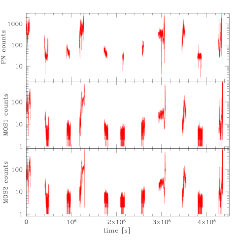
Figure 1: The time evolution of the background (total counts from the camera at energies $E\geq 8$ keV per 30 s bin) for the entire observation, separately plotted for each of the three detectors.

Table 1: Start time, exposure duration and livetime for the 11 individual exposures comprising the XMM-Newton campaign on L1551.

Obs. ID	Start time [yyyy-mm-dd hh-mm-ss UTC]				Elapsed time [ks]			Livetime [ks]
		PN	MOS1	MOS2	PN	MOS1	MOS2	PN	MOS1	MOS2
0201	2004-03-04	16:25:28	16:03:09	16:03:08	7.0	8.7	8.7	5.9	8.6	8.6
0301	2004-03-05	03:40:49	03:18:32	03:18:29	7.9	9.6	9.6	7.1	9.4	9.4
0401	2004-03-05	17:12:35	16:50:24	16:50:15	7.0	8.7	8.7	6.3	8.5	8.5
0501	2004-03-06	01:03:13	00:40:57	00:40:52	10.2	11.2	11.2	6.9	10.9	10.9
0601	2004-03-06	16:17:29	15:55:10	15:55:08	7.0	8.7	8.7	6.3	8.6	8.6
0701	2004-03-07	03:44:21	01:56:54	01:56:54	2.5	9.3	9.3	2.2	9.0	9.0
0801	2004-03-07	15:53:17	14:46:39	14:46:39	3.4	7.8	7.7	3.0	7.4	7.4
0901	2004-03-08	01:44:52	01:22:32	01:22:32	14.0	15.6	15.7	10.5	15.2	15.4
1001	2004-03-08	16:19:29	15:57:11	15:57:09	7.0	8.7	8.7	6.3	8.6	8.6
1101	2004-03-09	01:59:08	01:36:55	01:36:49	8.7	10.4	10.4	7.7	10.1	10.1
1201	2004-03-09	14:53:25	14:31:13	14:31:05	7.0	8.7	8.7	6.1	8.5	8.5

2.1 The merged data

Most of the known X-ray sources in L1551 are too weak to be visible in any of the eleven individual exposures. To try to detect fainter sources in the field, we stacked the individual exposures for each EPIC camera using the task merge in the SAS V6.0.0 pipeline. Prior to stacking, each exposure was filtered to reduce the background. To recover faint sources, the background must be reduced significantly below the high values present in the data; the 11 exposures were filtered (before merging) at a threshold level of 100 background counts per 30 sec bin for PN and 60 counts per 30 sec bin for MOS1 and MOS2. Table 2 summarizes the total (merged) live time before and after filtering. The PN camera was the one most affected by proton flares, and the restrictive filtering applied discards nearly half of the data. Thus, the remaining ’clean’ (low background) data in this observation is only $2/3$ for PN and just over $4/3$ for MOS1 and MOS2 of the clean time in the observation analyzed by FGM03 (even though the total exposure is twice as long). The observation is therefore not deeper than the one of FGM03. We used the merged observation to derive integrated spectra of 5 of the 7 bright sources (the ones that did not undergo a flare during the observation) and compared the resulting spectral parameters with the average value of the spectral parameters derived from the individual exposures. The good agreement between the two is an important verification of the validity of the spectra derived from the single exposures, despite the high background levels. An X-ray image produced from the merged data is shown in Fig. 2, together with a $K$-band 2MASS image.

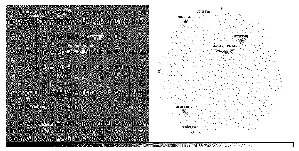
Figure 2: The left panel shows a mosaic of 2MASS $K$-band images of the region observed by XMM-Newton, while the right panel shows an X-ray image produced with the merged low-background data from all three EPIC detectors. The two images are on the same scale and have been registered (field size $\sim 30^{\prime}\times 30^{\prime}$ centered at 04:31:44 $+$18:10:29). The sources discussed in the paper have been labeled.

Table 2: Filtering thresholds (background counts per 30 sec bin) and livetime before and after filtering for the merged data for the three detectors. See text for more details.

Merged observations	Filtering [Counts]	Livetime [s]
Instrument	$E>8$ keV	Before	After
PN	100	68482	35053
MOS1	60	89521	73483
MOS2	60	89660	74994

3 Analysis of the individual sources

3.1 V826 Tau

V826 Tau is a K7 SB2 WTTS (Mundt et al., 1983). The separation between the two components is 0.06 AU (Jensen et al., 1994) and the period is 3.9 d (Mathieu, 1994). A photometric period of 3.7 d is known (Bouvier et al., 1995).

During the 2000 XMM-Newton observations (FGM03), the count rate of V826 Tau increased by $\simeq 50$% over the 50 ksec. Also during this 5-day monitoring campaign, V826 Tau showed significant variability on different time scales (Fig. 3) with a factor of $\simeq 2$ amplitude.

The spectral parameters for each exposure are summarized in Table 6. All PN spectra could be fit with absorbed 2T plasma models with metallicity frozen at 0.17 $Z_{\odot}$ (the best-fit value obtained by FGM03). The count rate variability is not linked to large variations in the spectral parameters. The average values of the spectral parameters and of the X-ray luminosity are compatible with the values determined by FGM03.

Figure 3: Right panel - From top to bottom: light curve of V826 Tau over the 5 days of monitoring (bin-time 3600 s), best-fit values for $N({\rm H})$  $kT_{1}$, $kT_{2}$ and for the ratio $E\!M_{1}/E\!M_{2}$. Left panel - light curve and best-fit values of spectral parameters for V826 Tau from the XMM-Newton observation of Sept. 2000 (from FGM03). All data are from the PN camera.

3.2 V827 Tau

V827 Tau is a K7 X-ray bright WTTS with a rotational period of 3.75 d (Bouvier et al., 1995). In the light curve (Fig. 4) a large flare lasting over one day is present with a count rate increase of a factor of 10. The emission before the flare varies significantly, by a factor of 3 over $\simeq$ 3 d.

Figure 4: From top to bottom: light curve of V827 Tau over the 5 days of monitoring (bin-time 3600 s) and best-fit values of $N({\rm H})$  $kT_{1}$, $kT_{2}$, and $E\!M_{1}/E\!M_{2}$ ratio (PN data), for the nine exposures not affected by the star’s flare. During the star’s flare the parameter values of the absorbed 3T-plasma fit are given. The PN data from XMM-Newton observation of 2000 are not given for this source because they were found unreliable after reprocessing with more recent SAS pipeline (see text for more details).

The best-fit spectral parameters are reported in Table 7. Excluding the flaring intervals, no significant spectral variations were present. The typical values ($N({\rm H})$ $\sim 0.1\times 10^{22}\leavevmode\nobreak\ {\rm cm^{-2}}$, $kT_{1}\sim 0.3$ keV, $kT_{2}\sim 1.2$ keV, and $Z=0.14\leavevmode\nobreak\ Z_{\odot}$) are very similar to the values derived in FGM03.

As in Table 7, the source intrinsic flux prior to the flare decreases slowly by a factor of $3$. The minimum X-ray luminosity is 4 times higher than the value reported by FGM03; however (as discussed in Sect. 2), reprocessing with the V6.0.0 software has shown that the data for this source were not properly reduced by the previous version of the SAS pipeline (probably because the source was very close to the edge of one of the chips); thus the X-ray luminosity value of V827 Tau given in FGM03 is most likely incorrect.

3.2.1 Flare analysis

To determine the flaring emission spectral parameters we subdivided the rise phase of the flare (Obs. 1001) into two segments (one for the rise phase and one for the peak). In order to separate the quiescent contribution from the flaring emission, we modeled the spectra with an absorbed 3T-plasma. The parameters of the first two components (representing the quiescent emission) were frozen to the values derived by simultaneously fitting four spectra during the quiescent phase (Obs. 0201, 0401, 0601, 0701, 0801). The values for the third component (the flaring emission) were then fitted. The results for this component are summarized in Table 3.

To derive the flare’s physical parameters we used the approach initially discussed by Reale et al. (1997) and since then applied to a variety of stellar flares. The calibration of the method for the XMM-Newton detectors, and a detailed explanation of the physics behind it can be found in Reale et al. (2004), to which the reader is referred. This approach allowed us to account properly for the presence of sustained heating during the flare decay, using the slope $\zeta$ of the flare decay in the $\log T$ vs. $\log\sqrt{E\!M}$ diagram. The semi-length of the flaring loop in this formulation is given by

$$L=\frac{\tau_{\rm LC}\sqrt{T_{\rm max}}}{\alpha F(\zeta)}\leavevmode\nobreak\ \leavevmode\nobreak\ \leavevmode\nobreak\ \leavevmode\nobreak\ \leavevmode\nobreak\ \leavevmode\nobreak\ \leavevmode\nobreak\ 0.35<\zeta\leq 1.6$$ (1)

where $\alpha=3.7\times 10^{-4}{\rm cm^{-1}s^{-1}K^{1/2}}$, $\tau_{\rm LC}$ is the $1/e$ folding time of the light curve decay, and $T_{\rm max}$ is the peak temperature of the plasma in the flaring loop. Then, $F(\zeta)$ and the relationship between $T_{\rm max}$ and the best-fit peak temperature $T_{\rm obs}$ are both functions that need to be separately determined for each X-ray detector, depending on its spectral response. For the EPIC PN,

$$F(\zeta)=c_{a}/(\zeta-\zeta_{a})+q_{a}$$ (2)

where $c_{a}=0.51\pm 0.03$, $\zeta_{a}=0.35\pm 0.01$, and $q_{a}=1.36\pm 0.18$. The range of validity corresponds to an impulsively heated flare ($\zeta=1.66$) and to very slow decays (strong sustained heating) corresponding to the locus of statics loops ($\zeta\leq 0.35$). The maximum temperature $T_{\rm max}$ is derived from $T_{\rm obs}$ as

$$T_{\rm max}=0.130T_{\rm obs}^{1.16}\leavevmode\nobreak\ \leavevmode\nobreak\ \leavevmode\nobreak\ \leavevmode\nobreak\ .$$ (3)

Figure 5: The evolution of the V827 Tau flare in the $\log T$ vs. $\log\sqrt{E\!M}$ plane.

The $\log T$ vs. $\log\sqrt{E\!M}$ diagram for the V827 Tau flare is shown in Fig. 5. Applying the above formalism to the flare, we derive $\tau_{\rm LC}=18.5$ ks and a slope $\zeta=0.73\pm 0.10$. Applying Eqs. 2 and 1, the resulting loop semi-length is $L=2.5-3.5,R_{\odot}$. Given its bolometric luminosity and temperature ($L_{\rm bol}=1.1L_{\odot}$, $T_{\rm eff}=4060$ K, as estimated by Briceño et al., 2002), the radius of V827 Tau is $R\simeq 2\,R_{\odot}$, so the loop has a size comparable to the star itself. Assuming for the loop a radius $r=0.1L$, typical of solar events, from the emission measure at the flare maximum one derives an electron density $n_{e}\simeq 1.3\times 10^{11}$ cm^-3, which is typical of the values found in the intense flares of YSOs (Favata et al., 2005). The corresponding equipartition magnetic field strength is $B\simeq 340$ G.

Table 3: Best-fit spectral parameters of the flaring component in V827 Tau during flare episode (Obs. 1001 has been subdivided into 2 segments). $Z=0.3\leavevmode\nobreak\ Z_{\odot}$ (frozen); units are $E\!M_{53}=10^{53}$ cm^-3. The parameters of the first two components were frozen to values derived by fitting four spectra during the quiescent phase (to the values $N({\rm H})$ $=0.09\times 10^{22}\leavevmode\nobreak\ {\rm cm^{-2}}$, $kT_{1}=0.36$ keV, $E\!M_{1}=3.60\times 10^{53}$ cm^-3, $kT_{2}=1.16$, $E\!M_{2}=6.64\times 10^{53}$ cm^-3, and $Z=0.11\leavevmode\nobreak\ Z_{\odot}$) as described in the text.

Obs.	$kT$	$E\!M$	$\chi^{2}$	$P$	Rate
	keV	$E\!M_{53}$			cts/s
1001A	4.27 $\pm$ 0.60	22.78 $\pm$ 0.97	0.90	0.71	1.57 $\pm$ 0.10
1001B	5.01 $\pm$ 0.26	95.75 $\pm$ 1.30	1.20	0.01	5.67 $\pm$ 0.09
1101	2.56 $\pm$ 0.09	15.26 $\pm$ 0.31	1.34	0.00	1.14 $\pm$ 0.02

3.3 V1075 Tau

V1075 Tau is a K7 binary WTTS with a 2.43 d rotational period (Bouvier et al., 1995). In the 2000 observation the V1075 Tau count rate decreased by a factor of $\simeq 2$ in about 30 ks. The FGM03 spectral analysis showed that, while the temperature did not change significantly, the absorption varied from $0.19\pm 0.03\times 10^{22}\leavevmode\nobreak\ {\rm cm^{-2}}$, when the source was more intense, to $0.08\pm 0.03\times 10^{22}\leavevmode\nobreak\ {\rm cm^{-2}}$ at the lower flux level.

The light curve of V1075 Tau is shown in Figure 6. Variability over a range of time scales is present, including a flare in the second exposure and an apparent modulation on a time scale of a couple of days.

Figure 6: Right panel - From top to bottom: light curve of V1075 Tau over the 5 days of monitoring (bin-time 3600 s) and best-fit values of $N({\rm H})$ and $kT$. Left panel - light curve and best-fit values of spectral parameters for V1075 from the XMM-Newton observation of Sept. 2000 (All are PN data). An absorbed 2T-plasma model was used for the spectral fits of the 2000 data. All data are from PN.

The spectral parameters are reported in Table 8. Given the moderate statistics, the data could be satisfactorily fit with a single temperature plasma. No changes in $N({\rm H})$ are visible, while $kT$ varies between 0.75 and 1.2 keV. Figure 7 shows a scatter plot between the spectral temperature and the count rate. The two are clearly correlated ($P=0.99993$ from a Wilcoxon test, Wilcoxon, 1945), showing that the variability is more likely intrinsic, rather than due to rotational modulation (which would probably result in a ’gray’ modulation, i.e. a spectral-independent change in the X-ray flux).

Figure 7: Count rate of V1075 Tau versus plasma temperature for the 11 exposures.

The spectral parameters for the merged spectrum ($N({\rm H})$$=0.10\pm 0.01\times 10^{22}$ cm^-2, $kT_{1}=0.37\pm 0.02$, $kT_{2}=1.00\pm 0.02$ and $Z=0.19\pm 0.03$) are similar to the FGM03 values, as is the X-ray luminosity ($L_{\rm X}=2.0\times 10^{30}$ erg s^-1).

3.4 V710 Tau A & B

V710 Tau is a CTTS+WTTS binary (Carkner et al., 1996) with spectral types M1 and M3 and masses 0.68 $M_{\sun}$ and 0.48 $M_{\sun}$ (Jensen & Akeson, 2003). With a projected separation of 3.2 arcsec, the system is not resolved by XMM-Newton. Its light curve is shown in Fig. 8. The system shows significant X-ray variability with the source counts varying by more than a factor of two. FGM03 found no evidence of variability from V710 Tau during the 50 ks 2000 XMM-Newton observations.

Due to the faintness of the source, PN and MOS data were fitted simultaneously with a single temperature model; Table 9 reports the spectral parameters. The merged PN spectrum of V710 Tau has sufficient statistics for a 2T fit. The spectral parameters ($N({\rm H})$$=0.19\pm 0.06\times 10^{22}$ cm^-2, $kT_{1}=0.30\pm 0.053$ $kT_{2}=0.93\pm 0.06$, $Z=0.2$ frozen) showed somewhat lower temperatures than in the 2000 observation ($kT_{1}=0.63\pm 0.05$, $kT_{2}=1.24\pm 0.10$, FGM03). However, the SAS V6.0.0 reprocessing of the FGM03 data flags most of the source photons as invalid (due to a row of hot pixels). The reprocessed MOS2 data of V710 Tau are, on the other hand, ‘clean’, and the best-fit to the 2000 data gives $N({\rm H})$$=0.30\pm 0.08\times 10^{22}$ cm^-2, $kT_{1}=0.38\pm 0.10$, $kT_{2}=1.12\pm 0.06$ ($P=0.06$), similar to the values of the current observation. The source X-ray luminosity from the merged data is $0.6\times 10^{30}$ erg s^-1, a factor of 2 lower than the 2000 value ($1.3\times 10^{30}$ erg s^-1).

Figure 8: From top to bottom: light curve of V710 Tau over the 5 days of monitoring (bin-time 3600 s, PN data) and best-fit values of $N({\rm H})$ and $kT$ (PN, MOS1 and MOS2 data). PN data from XMM-Newton observation of 2000 are not given for this source because they were found unreliable after reprocessing with more recent SAS pipeline (see text).

3.5 XZ Tau

XZ Tau is a binary CTTS with 0.3 arcsec separation (Haas et al., 1990), associated, together with HL Tau, with a complex set of bipolar jets and Harbig Haro outflows (Mundt et al., 1990). The spectral types are M2 and M3.5 for XZ Tau North and XZ Tau South, respectively (Hartigan & Kenyon, 2003). A photometric period of 2.6 days has been derived by Bouvier et al. (1995). They interpret this period as due to rotational modulation by a hot spot, 1500 K hotter than the photosphere and covering 1.2% of the stellar surface.

During the 2000 XMM-Newton observation (FGM03), the X-ray count rate increased by a factor of four in an approximately linear fashion over 50 ks. A time-resolved spectral analysis of the X-ray emission resulted in significant spectral changes, in particular a decrease in $N({\rm H})$ from $1.06\times 10^{22}$ cm^-2 to $0.26\times 10^{22}$ cm^-2. The temperatures increased from $kT_{1}=0.14$ keV and $kT_{2}=2.29$ keV to $kT_{1}=1.00$ keV and $kT_{2}=4.98$ keV (Table 5 in FGM03). The average spectrum was described well by a very low-metallicity plasma ($Z=0.007\leavevmode\nobreak\ Z_{\odot}$), with an X-ray luminosity $L_{\rm X}=1.3\times 10^{31}$ erg s^-1.

We reprocessed the data with SAS V6.0.0 and re-analyzed them, finding that the variation of $N({\rm H})$ reported by FGM03 may be spurious. The re-analysis shows that the spectral data for the first interval can be equivalently fit with two different solutions, one with the high $N({\rm H})$ reported by FGM03 and another with a low $N({\rm H})$ compatible with the later intervals. The two solution spaces are separated in the $\chi^{2}$ space well (as visible in Fig. 9) and both have an acceptable best-fit probability. However, ’Occam razor’ arguments lead us to prefer the one in which $N({\rm H})$ does not vary with respect to the rest. In fact, well-separated minima in the $\chi^{2}$ space are also present for the integrated 2000 spectrum.

The results of the spectral fits to the reprocessed 2000 data are given in Table 4 (replacing Table 5 of FGM03). The only spectral parameter that varies significantly over the 50 ks is the emission measure of the hotter component, which increases by a factor of five, with no appreciable increase in temperature. A very-similar phenomenon – a large ”slow” increase in the X-ray flux without significant change in the plasma temperature – was observed in the outbursting YSO V1674 Ori (Grosso et al., 2005). The average spectral parameters for the spectrum of the entire 50 ks observation resulting from this re-analysis are $\mbox{$N({\rm H})$}=0.24\pm 0.01$, $kT_{1}=0.83\pm 0.02$ keV $kT_{2}=4.09\pm 0.34$ keV, and $Z=0.22\pm 0.08$ for a corresponding intrinsic luminosity of $2.3\times 10^{30}$ erg s^-1, a factor of 6 lower than reported by FGM03, due to the change in $N({\rm H})$.

Figure 9: Contours of $\chi^{2}$ as a function of the spectral parameters $N({\rm H})$ and $Z$ for the fit to the 2000 spectrum of XZ Tau reprocessed with the V6.0.0 software, during the first time interval (the 50 ks observation was subdivided in three intervals). The $\chi^{2}$ space presents two well-separated minima that are both acceptable solutions. The cross indicates the solution implying no change in $N({\rm H})$.

Table 4: Best-fit spectral parameters for XZ Tau during three consecutive time intervals of the 2000 XMM-Newton observation. See the text for the details.

Time interval	$N({\rm H})$	$kT_{1}$	$kT_{2}$	$E\!M_{1}$	$E\!M_{2}$	$Z$	$\chi^{2}$	$P$
ks	$10^{22}\leavevmode\nobreak\ {\rm cm^{-2}}$	keV	keV	$10^{53}$ cm-6	$10^{53}$ cm-6	$Z_{\odot}$
0–20	$0.22\pm 0.04$	$0.84\pm 0.03$	$4.31\pm 1.34$	$0.32\pm 0.59$	$0.49\pm 0.10$	$0.40\pm 0.34$	1.33	0.06
20–40	$0.22\pm 0.021$	$0.82\pm 0.04$	$4.81\pm 0.77$	$0.69\pm 0.83$	$1.97\pm 0.57$	$0.20\pm 0.12$	0.79	0.95
40–54	$0.24\pm 0.02$	$0.83\pm 0.06$	$3.51\pm 0.38$	$0.62\pm 0.90$	$2.46\pm 0.28$	$0.24\pm 0.15$	0.94	0.63

The 2004 XMM-Newton light curve of XZ Tau is shown in Fig. 10. The data points relative to Obs. 0701 and Obs. 0801 have been omitted as they are strongly contaminated from the nearby HL Tau, which during this time is undergoing a large flare (see Sect. 6).

Table 10 summarizes the results of the spectral analysis of the PN data for the individual exposures; these were satisfactorily fit by an absorbed 1T plasma model. The spectral fits to the data for observations 0401 and 1101 can be improved by using a two-temperature plasma model (with larger error bars on the best-fit parameters); to allow a uniform comparison of the time variability we use the results of the 1T spectral fits.

Figure 10: Right panel - From top to bottom: light curve of XZ Tau over the 5 days of monitoring (bin-time 3600 s) and best-fit values of $N({\rm H})$ and $kT$ (Obs. 0701 and Obs. 0801 have been). Left panel - light curve and best-fit values of spectral parameters for XZ Tau from the XMM-Newton observation of Sept. 2000; for the spectral fits of the 2000 data an absorbed 2T-plasma model was used. All data are from PN.

Figure 10 shows the best-fit values of $N({\rm H})$ and $kT$. While variability of a factor of $\simeq 2$ in the count rate is present, no significant spectral variations are detected. A spectral fit to the merged data for XZ Tau (with the exclusion of Obs. 0701, 0801, and 0901, to prevent contamination from the HL Tau flare) yields $N({\rm H})$$=0.19\pm 0.03\times 10^{22}$ cm^-2, $kT_{1}=0.34\pm 0.03$, $kT_{2}=1.22\pm 0.07$, and $Z=0.14\pm 0.04$ ($P=0.02$, $\Delta E=0.3-3.0$ keV) for a corresponding luminosity of $1.3\times 10^{30}$erg s^-1(a factor of 2 lower than in 2000).

The plasma temperature during the 2004 observation is significantly lower than in 2000, with no evidence of the hot ($T\simeq 4$ keV) component clearly present in the 2000 data. Visual inspection of the two spectra (top panel of Fig. 11, which plots both spectra reprocessed with the standard SAS V6.0.0 pipeline) shows that indeed the high-energy tail clearly visible in the 2000 spectrum has weakened significantly. For comparison, the bottom panel of Fig. 11 shows the 2000 and 2004 spectra of V826 Tau, for which no differences are visible, allowing us to exclude e.g. problems in the background filtering.

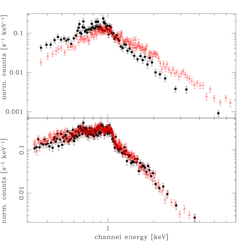
Figure 11: Spectra of XZ Tau (top panel) and V826 Tau (bottom panel) from the merged PN data from the 2004 monitoring campaign (filled circles) and from the 2000 observations (open triangles). While the V826 Tau spectra are almost identical, the hard component present in 2000 in XZ Tau is no longer visible.

XZ Tau is the only star in the sample showing substantial spectral changes from 2000 to 2004. In 2000 XZ Tau had a hotter X-ray spectrum than in either 2001 or in 2004: the 2000 spectrum indicates $kT_{1}=0.83\pm 0.02$ keV and $kT_{2}=4.09\pm 0.34$ keV, while the present (2004) data indicate $kT_{1}=0.3-0.7$ keV and $kT_{2}=1.0-1.5$ keV, which are very similar to the values derived from the July 2001 Chandra observation (FGM03), $kT_{1}=0.65\pm 0.03$ and $kT_{2}=1.56\pm 0.12$. The light curve of the 2000 observation shows no obvious evidence of flaring (which would justify the higher temperature); slow variability is present, starting from a lower value than any of the present observations and rising to a value similar to the 2004 one.

Ground-based $UVBR$ photometry of XZ Tau from 1962 to 1993 detected variations of $\geq 2$ mag (Herbst et al., 1994), integrated on both components of the binary system. Coffey et al. (2004) monitored XZ Tau and its outflows from 1995 till 2001 using HST, which resolves the binary. XZ Tau South ($R\simeq 13.5$) displays moderate variability ($\Delta R\leq 0.3$ mag), while XZ Tau North (the suspected source of the outflow) displays dramatic variations: in Jan. 1995 its magnitude was $R=14.93$, fading by about 1 mag until 1998 and thereafter brightening by 3 mag, so that by Feb. 2001 XZ Tau North was actually the brighter star (also visible in Fig. 1 of Coffey et al., 2004). This behavior suggests that XZ Tau North is an EXor. EXors, named after their prototype EX Lupi, are a loosely defined class of eruptive CTTS that periodically undergo outbursts from the UV to the optical. Although increases by several magnitudes with rise times of up to a few years have been recorded (Herbig, 1989), the changes in these YSOs are not as extreme as in FU Ori stars (EXor spectra during outburst, for example, continue to resemble the ones of T Tauri stars). This phenomenon is thought to be due to major increases in the underlying disk accretion rate; however, the number of known EXors is relatively small and the class remains poorly defined.

While the HST data presented by Coffey et al. (2004) extend only to Feb. 2001, a number of more recent HST observations are present in the public archive, which can help to determine whether the outburst that was ongoing at the time of the 2000 observation has lasted into the 2001 Chandra and 2004 XMM-Newton observations. We have located a number of unpublished observations in the HST archive, which we extracted and inspected. While a full photometric analysis of these observations is beyond the scope of the present work, even simple visual inspection of the images allows assessment of the luminosity of XZ Tau N (the component found to strongly vary by Coffey et al., 2004) compared to the more stable XZ Tau S. We have chosen four HST observations (all taken in red filters) to be as close as possible in time to the X-ray observations. A zoom centered on the resolved XZ Tau binary is shown in Fig. 12. The first three observations are all from the WFPC2 camera, in the F675W filter, while the last (2004) observation is taken with the ACS camera, with the FR656N filter. The XMM-Newton observation of FGM03 took place in Sept. 2000 between the HST observation of Feb. 2000, when the brightening of XZ Tau N was already going on (Coffey et al., 2004), and the HST observation of Feb. 2001, when the outburst was clearly visible. The outburst, however, did not appear to be long lasting: one year later (Feb. 2002) the outburst was already finished, with XZ Tau N back to being fainter than the S component. In early 2004 it was, if anything, even fainter than the S component. The Chandra observation of July 2001 fell between the early 2001 and early 2002 HST observations, and the present XMM-Newton campaign (4–9 Mar. 2004) is very close in time to the 2004 HST observation.

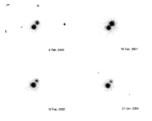
Figure 12: A mosaic of HST images of the XZ Tau binary taken between 2000 and 2004 (field size $4^{\prime\prime}\times 3^{\prime\prime}$ centered on XZ Tau, at 04:31:40.07 $+$18:13:57.1). While during the outburst episode of 2001 XZ Tau N was the brightest component, 1 year later it had faded back to being the fainter component, and by early 2004 (when the XMM-Newton observations discussed here have been taken) the S component is much stronger. The 2000, 2001, and 2002 images are from the WFPC2 camera, in the F675W filter, while the 2004 is from the ACS camera in the FR656N filter.

While the X-ray and optical observations are not simultaneous and the binary system is not resolved by XMM-Newton, the temporal proximity of the optical outburst of XZ Tau N and of the X-ray spectral hardening (as well as of the peculiar variability observed in 2000) is very suggestive of a connection between the two phenomena. Such a connection has been well-documented for V1647 Ori by Kastner et al. (2004), who reports a significant increase in spectral hardness near the peak of the optical outburst, as well as a surge of X-ray flux. Moreover, as already mentioned, the outbursting source V1647 Ori also displays the type of ‘slow’ variability observed for XZ Tau in 2000 (Grosso et al., 2005).

3.6 HL Tau

HL Tau, at about 24 arcsec from XZ Tau, is a K7 embedded young stellar object, often considered a prototype very young solar-mass star (0.5$-$0.7 $M_{\sun}$), with a circumstellar disk that resembles the solar nebula at the early stages of planet formation (Men’shchikov et al., 1999). Together with XZ Tau, it is associated with bipolar jets and Herbig-Haro outflows (Mundt et al., 1990).

Although initially classified as a CTTS, it is now thought to be in a transition phase from protostar (Class I object) to CTTS. An infalling envelope around the source was found by Hayashi et al. (1993), who reported evidence of non-steady accretion. Close et al. (1997) found that to reproduce the observed SED, the central source in HL Tau is required to be a very young ($\sim 10^{5}$ yr) PMS surrounded by an active accretion disk and accreting at the rate of $5\times 10^{-6}\leavevmode\nobreak\ M_{\sun}$ yr^-1.

Ground-based photometry of HL Tau from 1973 to 1993 has shown variations of 0.5 to 2 mag in $UVBR$ (Herbst et al., 1994). During the 2000 XMM-Newton 50ks observations HL Tau did not display significant variability, while in the 2001 80 ks Chandra observation (Bally et al., 2003), it underwent a small short duration flare (Fig. 6 in FGM03). As shown in Figure 13 in the present observation, HL Tau underwent a large ($\times\leavevmode\nobreak\ 25$ in count rate) flare which decays over about two days.

The best-fit spectral parameters are reported in Table 11. Given the low statistics of individual spectra, the metal abundance was frozen to $Z=0.6\leavevmode\nobreak\ Z_{\odot}$, the value determined in 2000 by FGM03. Outside of the flare the spectral parameters do not vary significantly and their average values (see below) are similar to the 2000 values (FGM03), as is the X-ray luminosity ($1.5\times 10^{30}$ erg s^-1).

Figure 13: Right panel - From top to bottom: light curve of HL Tau over the 5 days of monitoring (bin-time 3600 s) and best-fit values of $N({\rm H})$ and $kT$. Left panel - light curve and best-fit values of spectral parameters for HL Tau from the XMM-Newton observation of Sept. 2000.

Table 5: Best-fit spectral parameters of the flaring component in HL Tau. Units are $N_{22}=10^{22}\leavevmode\nobreak\ {\rm cm^{-2}}$, $E\!M_{53}=10^{53}$ cm^-3 and $F_{-13}=10^{-13}$ erg cm^-2 s^-1.

Obs.	$N({\rm H})$	$kT$	$E\!M$	$Z$	$\chi^{2}$	$P$	Rate
	$N_{22}$	keV	$E\!M_{53}$	$Z_{\odot}$			cts/s
0701	3.40 $\pm$ 0.27	8.79 $\pm$ 2.50	14.01 $\pm$ 1.87	0.48 $\pm$ 0.19	0.75	0.90	0.48 $\pm$ 0.01
0801	3.73 $\pm$ 0.33	3.86 $\pm$ 0.62	15.88 $\pm$ 3.08	0.26$\pm$ 0.11	0.87	0.73	0.35 $\pm$ 0.01
0901	4.29 $\pm$ 0.35	7.02 $\pm$ 1.51	9.55 $\pm$ 1.57	0.27$\pm$ 0.11	0.88	0.71	0.26 $\pm$ 0.01

To derive the flaring emission spectral parameters, we applied the same procedure as for V827 Tau. The quiescent spectral parameters are $N({\rm H})$$=2.43\times 10^{22}\leavevmode\nobreak\ {\rm cm^{-2}}$, $kT=3.10$ keV, $E\!M=1.40\times 10^{53}$ cm^-3, and $Z=0.6\leavevmode\nobreak\ Z_{\odot}$, and the resulting spectral parameters for the flaring component are listed in Table 5. The event shows a peculiar evolution, with a monotonically decaying light curve associated with a highly irregular temperature evolution. The temperature has two well-defined peaks above 7 keV separated by a deep minimum at about 3 keV. The temperature evolution suggests that this is the combination of two flares, probably physically related to each other but occurring in independent coronal structures. This kind of evolution has been predicted by modeling two independent flares by Reale, Güdel, Peres, & Audard (2004).

In order to support this hypothesis, we modeled the event by combining two flares computed with detailed hydrodynamic modeling of plasma confined in a coronal loop. The light curve decay time suggests long flaring structures (e.g. Serio et al., 1991), so that we considered each model flare to be identical to the one used to describe one of the flares observed during the COUP campaign (Favata et al., 2005) in detail. We assumed that each flare occurs in a coronal loop with a constant cross-section and half-length $L=10^{12}$ cm, symmetric around the loop apex. Both flares were triggered by injecting a heat pulse in the loop, which was initially at a temperature of $\simeq 20$ MK. This heat pulse is symmetrically deposited at the loop footpoints with a Gaussian spatial distribution of intensity 10 erg cm^-3 s^-1 and width $10^{10}$ cm (1/100 of the loop half-length). After 20 ks the heat pulse was switched off completely. From the evolution of the plasma density and temperature along the loop computed with the Palermo-Harvard hydrodynamic loop model (Peres et al., 1982, Betta et al., 1997), we synthesized the corresponding EPIC spectra of the loop throughout the flare, deriving a light curve and the evolution of temperature.

To model the HL Tau event we duplicated, the resulting light curve and temperature evolution with a time shift. The two flares are identical flares, except for a normalization factor, which represents the loop cross-section and does not enter explicitly in the hydrodynamic modeling. The second flare has a normalization factor of 0.3 (i.e. a correspondingly smaller cross-section) and it starts 60 ks after the first. We summed the resulting two asynchronous sequences of flare spectra and obtained a single sequence of spectra, which we integrated to derive a single light curve and fit with single temperature EPIC model spectra. Figure 14 shows the resulting light curve and temperature evolution as compared to those obtained from the data. The model temperatures in the first flare are somewhat higher than the observed one, but the main flare characteristics, i.e. the monotonic light curve and the temperature dip, are reproduced by the double-flare model well – although the model is not unique.

Since no constraint can be derived from the data, each of the two flares was modeled with no significant residual heating present during the flare decay (e.g. Reale et al., 1997). Such modeling implies very large flaring structures, similar to the ones found in ONC YSOs by Favata et al. (2005) – where the data allowed investigation of the presence of sustained heating. Such large structures, with $L\simeq 5\,R_{*}$, have only been found in YSOs, and were interpreted by Favata et al. (2005) as linking the star to the accretion disk, i.e. as being the magnetic structures supporting the magnetospheric accretion. In addition to the evidence from the ONC YSOs, HL Tau is the first Taurus YSO in which such large flaring structures have been detected. We cannot a priori exclude that shorter loops with sustained heating in the decay may also reproduce the features of this flare. However, the long delay of the model flares required to reproduce the distant temperature peaks suggests that very large structures must be involved in the flare (Reale et al., 2004).

Figure 14: Top panel - The observed light curve for HL Tau (asterisks), together with the light curve predicted by the flare modeling described in the text. Bottom panel - The observed temperature evolution of the HL Tau flare, together with the double-peaked temperature evolution predicted by the same flare modeling. The model is obtained by combining two models of $2\times 10^{12}$ cm-long flaring loops (dotted and dashed lines). The two models are identical, except for the cross-section of the flaring loops and for the start time (60 ks delay).

3.7 HD 285845

Unlike the other stars in the present study, HD 285845 (an active binary system) is not a member of the star-forming region, on the basis of its radial velocity and proper motion (Walter et al., 1988). The primary spectral type is G8, and Schneider et al. (1998) report a separation of 73 mas and a magnitude difference of 1.19 mag.

In the 2000 observation, HD 285845 showed significant variability, and similar behavior is present in the present data set (Fig. 15). Table 12 summarizes the best-fit spectral parameters. Notwithstanding the significant count-rate variability, the spectral parameters show little variation in time.

Figure 15: Right panel - From top to bottom: light curve of HD285845 over the 5 days of monitoring (bin-time 3600 s), best-fit values of $N({\rm H})$  $kT_{1}$, $kT_{2}$ and $E\!M_{1}/E\!M_{2}$ ratio. Left panel - light curve and best-fit values of spectral parameters from the XMM-Newton observation of Sept. 2000 (All are PN data).

4 Temporal variability

All the stars in the sample show significant variability, although with different characteristics. To quantify this variability we computed the normalized cumulative distributions of the amplitude variability. These represent the fraction of time that a source spends in a state with the flux larger than a given value, expressed in terms of a given a normalization value, which can be the minimum count rate, the median count rate, etc. For the present sample we took as normalization value the count rate above which a source spends 90% of the time; this is less sensitive to noise fluctuations than the real minimum.

Figure 16 shows the distribution for the stars in our sample (except V710 Tau for which the count rate uncertainties are too large). Some sources (V826 Tau, HD285845 and XZ Tau) show mostly low-amplitude variability, in which less than 30% of the time is spent in a state 1.3$-$1.5 above the minimum. On the other hand, V827 Tau and HL Tau spend more than 60% of the time in such a state, while V1075 Tau shows intermediate behavior. The differences between V827 Tau and HL Tau are not due to the large flares present in their light curves, as the flare points affect only the 10 bins relative to the highest count rate, while the low-variability tails of the distributions are also significantly different.

Kolmogorov-Smirnov tests for the cumulative distributions of various pairs of sources also indicate the presence of the different behaviors. While this would suggest differences in the X-ray emission processes, the two groups are heterogeneous, and both contain CTTS and WTTS, so that a simple interpretation in terms of e.g. accreting vs. non-accreting sources is not possible.

Figure 16: Normalized cumulative count-rate distribution for all the star considered apart from V710 Tau.

5 Discussion

The X-ray monitoring observations of the L1551 star-forming complex discussed here, in conjunction with the 2000 XMM-Newton observations (FGM03) and the 2001 Chandra observations (Bally et al., 2003), has allowed us to probe the X-ray intensity and spectral variability from six YSOs (both CTTS and WTTS), on a variety of time scales, from hours to days to years.

Most stars in the sample show X-ray variability at an amplitude of a factor of $\simeq 2$ on time scales of a few days. In the WTTS V1075 Tau, the source count rate varies on time scales similar to its optically derived rotational period, which would be compatible with rotational modulation (as observed in YSO in the ONC, Flaccomio et al., 2005), but the significant correlation with spectral variability would appear to point to intrinsic variations. Plasma temperature variations of the order of 20% on similar time scales are also present, and in some cases they appear to be correlated with the intensity (e.g. for V1075 Tau).

Again XZ Tau emerges as a peculiar source. While the short-term (day scale) spectral variability of XZ Tau is not linked to variations in the absorbing column density, as originally speculated by FGM03 – reprocessing and reanalysing the original 2000 XMM-Newton data showing that the variation reported by FGM03 was probably spurious – this is the only source in the sample to show significant long-term changes in its spectrum.

The spectrum of XZ Tau observed with XMM-Newton in 2000 had a significant hard component ($T\simeq 4$ keV), which was not visible in the 2001 Chandra data and is not present in the 2004 XMM-Newton data and both are compatible with a hard component of at most 1.5 keV. The difference between the two spectral states is very well visible in Fig. 11. The X-ray spectral hardening takes place close in time to the strong optical outburst of the N component of the binary. While the data by Coffey et al. (2004), who reported the outburst, only cover its beginning, our own inspection of new HST data indicates that the outburst was not long-lived, with the source returning to its state fainter than XZ Tau S by early 2002, one year after the early 2001 peak.

Finally, while (Fig. 10) the count rate varied smoothly between 0.04 and 0.22 cts/sec during the 2000 observation, during the 2004 campaign it never decreased below 0.12 cts/sec (with a peak value of $\simeq 0.35$ cts/sec), again showing the source to be in a different state.

The binary system XZ Tau is not resolved in the X-ray, therefore one cannot exclude that XZ Tau S may have been the dominant X-ray source, at one or all the epochs at which it was observed. Nevertheless the observed phenomena are very reminiscent of the spectral hardening and variability observed in the outbursting source, V1647 Ori (Kastner et al., 2004; Grosso et al., 2005), so that it seems reasonable to interpret the X-ray spectral changes and variability of XZ Tau as connected with the outburst of XZ Tau N. The potential physical mechanism causing the significantly harder X-ray spectrum (with a somewhat lower emission level) during the optical outburst is difficult to assess. While the optical outburst is naturally interpreted as an accretion outburst (with the optical luminosity due to increased luminosity of the accretion shock), why this should cause a hot plasma component to appear in the star is not clear. Indeed, accreting YSOs in the COUP sample are statistically less X-ray luminous than non-accreting ones (Preibisch et al., 2005) and less prone to show flares from large magnetic structures (Favata et al., 2005).

The temperature of the hot component observed in XZ Tau in 2000 is such that it cannot be due to simple accretion-driven emission, as the shock temperature in a low-mass T Tau star is too low . Its early M spectral type corresponds, at this age, to a typical mass $M\simeq 0.5\,M_{\odot}$ and to a radius $R\simeq R_{\odot}$, resulting (Calvet & Gullbring, 1998) in a peak shock temperature $T\simeq 0.2$ keV.

Nevertheless, a heating of the plasma during an accretion outburst in XZ Tau N would be consistent with the observed high X-ray plasma temperatures in accreting objects, like Class I sources. In a study of the $\rho$ Oph region, Imanishi et al. (2003) find that Class I sources have a higher $\langle kT\rangle$ (sometimes exceeding 5 keV) on average than Class II-III sources. This is confirmed by the study of $\rho$ Oph by Ozawa et al. (2005) that finds an evolutionary trend from Class I sources showing higher temperature and larger absorption to Class II and III sources showing lower temperatures and smaller extinction. In the present sample the only star with a consistently high plasma temperature ($kT=2.5-4$ keV) is HL Tau, a PMS in the transition phase between Class I and Class II, which is still undergoing substantial accretion.

Apart from XZ Tau, no significant variations in the activity level of our target YSOs on time scales of four years is observed. While evidence of solar-like cyclical variation is accumulating (Favata et al., 2004; Robrade et al., 2005) for low- and intermediate-activity stars, long-term variations (whether cyclical or not) in the activity levels of high-activity stars (including YSOs) do not seem to be present.

Although the data do not allow a fully detailed modeling, the double-temperature peaked flaring event observed in HL Tau most likely originates in very large magnetic structures, similar to the ones observed in ONC YSOs. Such structures, postulated by the magnetospheric accretion model, probably link the stellar photosphere to the inner rim of the accretion disk. In the ONC sample only objects that are currently not accreting were shown to have very large flaring magnetic structures (Favata et al., 2005). The only active accretor present in the sample showed flares confined to small structures, similar to normal coronal flares. HL Tau (with the caveat linked to the limited spectral information available) would provide a counter-example to the scheme observed in the ONC, being the first strongly accreting YSO with large flaring magnetic structures.

6 Conclusions

The present monitoring campaign has allowed us to study the luminosity and spectral variability of the X-ray emission from a number of YSO over a range of time intervals, sampling in particular the variability over a 5-day span, as well as over 4 years.

While most YSOs show a remarkably constant level of activity over the 4-year span sampled, XZ Tau has shown significant spectral variability apparently in conjunction with an optical outburst of the N component of the binary system, which took place in 2000. The role of accretion in the X-ray of YSOs is a matter of current debate, with a few spectral observations indicating differences in the density and UV environment of the plasma in a few accreting YSOs, and with a number of authors speculating on the possible relationship between accretion and coronal heating. Kastner et al. (2004) and Grosso et al. (2005) report on spectral hardening and enhanced variability in V1647 Ori in conjunction with a well-documented optical/IR outburst, which provides evidence that strongly enhanced high-energy emission can occur as a consequence of high accretion rates. The significant spectral changes detected here supply similar evidence.

Table 6: Best-fit spectral parameters of the PN data for the eleven exposures of V826 Tau. $E\!M$ is the emission measure, $P$ the null-hypothesis probability of the fit,and $F_{\rm X}$ Intr. the ”unabsorbed” X-ray flux. Units are $N_{22}=10^{22}\leavevmode\nobreak\ {\rm cm^{-2}}$, $E\!M_{53}=10^{53}$ cm^-3, and $F_{-13}=10^{-13}$ erg cm^-2 s^-1. The metallicity was frozen at $Z=0.17\leavevmode\nobreak\ Z_{\sun}$. The spectral fits were carried out in the energy range 0.3–7.5 keV.

Obs.	$N({\rm H})$	$kT_{1}$	$E\!M_{1}$	$kT_{2}$	$E\!M_{2}$	$\chi^{2}$	$P$	$F_{\rm X}$	$F_{\rm X}$ Intr.
	$N_{22}$	keV	$E\!M_{53}$	keV	$E\!M_{53}$			$F_{-13}$	$F_{-13}$
0201	0.17 $\pm$ 0.04	0.28 $\pm$ 0.02	6.51 $\pm$ 3.74	1.07 $\pm$ 0.06	3.74 $\pm$ 0.68	1.01	0.45	11.52	24.51
0301	0.06 $\pm$ 0.03	0.39 $\pm$ 0.06	1.19 $\pm$ 0.83	1.04 $\pm$ 0.05	1.65 $\pm$ 0.32	1.16	0.19	6.33	8.30
0401	0.10 $\pm$ 0.03	0.35 $\pm$ 0.04	2.06 $\pm$ 1.23	1.19 $\pm$ 0.06	2.46 $\pm$ 0.36	1	0.47	8.34	12.72
0501	0.15 $\pm$ 0.05	0.26 $\pm$ 0.02	6.04 $\pm$ 4.84	0.89 $\pm$ 0.07	3.49 $\pm$ 0.81	1.01	0.42	10.60	22.20
0601	0.10 $\pm$ 0.02	0.31 $\pm$ 0.02	3.51 $\pm$ 1.49	1.2 $\pm$ 0.04	4.88 $\pm$ 0.41	1.16	0.12	15.72	23.66
0701	0.15 $\pm$ 0.06	0.29 $\pm$ 0.04	3.70 $\pm$ 3.86	0.97 $\pm$ 0.08	2.62 $\pm$ 0.78	0.49	0.96	7.90	15.69
0801	0.01 $\pm$ 0.03	0.44 $\pm$ 0.29	0.55 $\pm$ 0.74	1 $\pm$ 0.07	2.25 $\pm$ 0.70	1.02	0.44	8.81	9.06
0901	0.13 $\pm$ 0.04	0.26 $\pm$ 0.03	4.23 $\pm$ 2.80	0.83 $\pm$ 0.05	3.18 $\pm$ 0.85	1	0.51	9.65	17.98
1001	0.11 $\pm$ 0.04	0.31 $\pm$ 0.03	3.06 $\pm$ 2.07	0.98 $\pm$ 0.06	2.73 $\pm$ 0.56	0.95	0.62	9.02	15.15
1101	0.15 $\pm$ 0.03	0.28 $\pm$ 0.02	4.50 $\pm$ 2.18	0.96 $\pm$ 0.04	3.18 $\pm$ 0.42	1.06	0.34	9.44	18.80
1201	0.11 $\pm$ 0.03	0.27 $\pm$ 0.03	2.83 $\pm$ 1.80	0.94 $\pm$ 0.05	2.93 $\pm$ 0.45	0.87	0.79	8.92	14.92

Table 7: Best-fit spectral parameters of the PN data for the eleven exposures of V827 Tau. $E\!M$ is the emission measure, $P$ the null-hypothesis probability of the fit, and $F_{\rm X}$ Intr. the ”unabsorbed” X-ray flux.

Units are $N_{22}=10^{22}\leavevmode\nobreak\ {\rm cm^{-2}}$, $E\!M_{53}=10^{53}$ cm^-3, and $F_{-13}=10^{-13}$ erg cm^-2 s^-1.The spectral fits were carried out in the energy range 0.3–7.5 keV.

Obs.	$N({\rm H})$	$kT_{1}$	$Z$	$E\!M_{1}$	$kT_{2}$	$E\!M_{2}$	$\chi^{2}$	$P$	$F_{\rm X}$	$F_{\rm X}$ Intr.
	$N_{22}$	keV	$Z_{\odot}$	$E\!M_{53}$	keV	$E\!M_{53}$			$F_{-13}$	$F_{-13}$
0201	0.13 $\pm$ 0.03	0.26 $\pm$ 0.04	0.05 $\pm$ 0.02	12.89 $\pm$ 11.85	1.19 $\pm$ 0.12	17.47 $\pm$ 3.31	1.04	0.35	35.33	55.92
0301	0.09 $\pm$ 0.02	0.32 $\pm$ 0.02	0.22 $\pm$ 0.06	4.67$\pm$ 2.61	1.48 $\pm$ 0.09	9.69 $\pm$ 1.40	1.27	0.01	43.09	45.96
0401	0.11 $\pm$ 0.02	0.30 $\pm$ 0.03	0.10 $\pm$ 0.04	5.55 $\pm$ 4.27	1.18 $\pm$ 0.09	7.92 $\pm$ 1.80	1.01	0.45	19.98	30.02
0501	0.06 $\pm$ 0.03	0.39 $\pm$ 0.07	0.20 $\pm$ 0.08	2.16 $\pm$ 1.94	1.30 $\pm$ 0.07	5.10 $\pm$ 1.62	0.91	0.78	18.54	22.80
0601	0.08 $\pm$ 0.02	0.42 $\pm$ 0.12	0.10 $\pm$ 0.03	2.07 $\pm$ 2.01	1.09 $\pm$ 0.07	5.85 $\pm$ 4.85	0.80	0.90	15.00	20.17
0701	0.06 $\pm$ 0.05	0.43 $\pm$ 0.14	0.23 $\pm$ 0.12	1.70 $\pm$ 2.37	1.28 $\pm$ 0.11	3.51 $\pm$ 1.71	1.00	0.45	13.91	17.43
0801	0.09 $\pm$ 0.04	0.36 $\pm$ 0.07	0.17 $\pm$ 0.09	2.82 $\pm$ 3.32	1.32 $\pm$ 0.10	4.05 $\pm$ 1.49	1.10	0.31	13.80	19.02
0901	0.15 $\pm$ 0.05	0.27 $\pm$ 0.04	0.12 $\pm$ 0.06	6.21 $\pm$ 7.82	1.09 $\pm$ 0.15	6.30 $\pm$ 2.84	0.99	0.51	14.91	26.25
1001	0.04 $\pm$ 4.90E-03	0.79 $\pm$ 0.06	0.93 $\pm$ 0.14	0.78 $\pm$ 0.31	5.08 $\pm$ 0.24	29.86 $\pm$ 1.11	0.99	0.57	200.39	219.25
1101	0.05 $\pm$ 6.33E-03	0.76 $\pm$ 0.02	0.50 $\pm$ 0.09	2.42 $\pm$ 0.81	3.04 $\pm$ 0.14	13.65 $\pm$ 0.81	1.03	0.37	80.36	89.18
1201	0.11 $\pm$ 0.02	0.33 $\pm$ 0.03	0.14 $\pm$ 0.06	5.14 $\pm$ 4.03	1.45 $\pm$ 0.13	8.48 $\pm$ 1.68	1.19	0.08	25.53	36.67

Table 8: Best-fit spectral parameters of the PN data for the eleven exposures of V1075 Tau. In this case $Z$ was frozen at 0.15 $Z_{\odot}$, the value derived for this source from the XMM-Newton observation of L1551 of 2000 (FGM03). $E\!M$ is the emission measure, $P$ the null-hypothesis probability of the fit, and $F_{\rm X}$ Intr. the ”unabsorbed” X-ray flux. Units are $N_{22}=10^{22}\leavevmode\nobreak\ {\rm cm^{-2}}$, $E\!M_{53}=10^{53}$ cm^-3, and $F_{-13}=10^{-13}$ erg cm^-2 s^-1.The spectral fits were carried out in the energy range 0.3–7.5 keV.

Obs.	$N({\rm H})$	$kT$	$E\!M$	$\chi^{2}$	$P$	$F_{\rm X}$	$F_{\rm X}$ Intr.
	$N_{22}$	keV	$E\!M_{53}$			$F_{-13}$	$F_{-13}$
0201	0.06 $\pm$ 0.03	0.77 $\pm$ 0.04	2.04 $\pm$ 0.50	0.81	0.86	4.90	6.37
0301	0.07 $\pm$ 0.01	1.05 $\pm$ 0.02	5.30 $\pm$ 0.38	1.62	1.8E-4	13.06	17.48
0401	0.04 $\pm$ 0.02	0.95 $\pm$ 0.04	2.64 $\pm$ 0.35	0.94	0.6	7.32	8.61
0501	0.07 $\pm$ 0.03	0.88 $\pm$ 0.07	2.18 $\pm$ 0.54	1.09	0.25	5.15	7.05
0601	0.06 $\pm$ 0.02	0.94 $\pm$ 0.04	2.43 $\pm$ 0.35	0.84	0.76	6.16	7.91
0701	0.03 $\pm$ 0.03	1.03 $\pm$ 0.05	3.26 $\pm$ 0.59	1.51	0.09	9.17	10.15
0801	0.01 $\pm$ 0.03	0.76 $\pm$ 0.04	2.11 $\pm$ 0.54	0.89	0.61	6.24	6.56
0901	0.03 $\pm$ 0.03	0.76 $\pm$ 0.04	1.96 $\pm$ 0.44	0.99	0.53	5.19	6.13
1001	0.08 $\pm$ 0.03	0.75 $\pm$ 0.04	2.52 $\pm$ 0.57	1.41	0.02	5.41	7.81
1101	0.05 $\pm$ 0.01	1.05 $\pm$ 0.03	2.35 $\pm$ 0.26	1.96	9.2E-5	6.36	7.77
1201	0.11 $\pm$ 0.04	0.64 $\pm$ 0.04	2.33 $\pm$ 0.67	1.35	0.08	4.20	6.83

Table 9: Spectral parameters derived from simultaneously fitting PN, MOS1, and MOS2 data for the eleven exposures of V710 Tau. In this case $Z$ was frozen at 0.2 $Z_{\odot}$. $E\!M$ is the emission measure, $P$ the null-hypothesis probability of the fit, and $F_{\rm X}$ Intr. the ”unabsorbed” X-ray flux. Units are $N_{22}=10^{22}\leavevmode\nobreak\ {\rm cm^{-2}}$, $E\!M_{53}=10^{53}$ cm^-3, and $F_{-13}=10^{-13}$ erg cm^-2 s^-1. The spectral fits were carried out in the energy range 0.3–7.5 keV.

Obs.	$N({\rm H})$	$kT$	$E\!M$	$\chi^{2}$	$P$	$F_{\rm X}$	$F_{\rm X}$ Intr.
	$N_{22}$	keV	$E\!M_{53}$			$F_{-13}$	$F_{-13}$
0201	0.24 $\pm$ 0.23	0.90 $\pm$ 0.24	0.56 $\pm$ 0.52	0.9	0.63	0.98	1.86
0301	0.43 $\pm$ 0.10	0.83 $\pm$ 0.08	1.15 $\pm$ 0.58	1.35	0.14	1.31	3.71
0401	0.22 $\pm$ 0.13	0.78 $\pm$ 0.10	0.54 $\pm$ 0.40	0.71	0.76	0.91	1.74
0501	0.71 $\pm$ 0.27	0.41 $\pm$ 0.24	4.24 $\pm$ 12.66	1.35	0.05	1.01	9.93
0601	0.24 $\pm$ 0.12	0.78 $\pm$ 0.09	0.76 $\pm$ 0.49	1.12	0.34	1.23	2.39
0701	0.31 $\pm$ 0.37	0.60 $\pm$ 0.73	0.82 $\pm$ 3.73	0.71	0.54	0.86	2.03
0801	0.46 $\pm$ 0.21	0.72 $\pm$ 0.16	1.12 $\pm$ 1.26	0.95	0.48	1.07	3.16
0901	0.10 $\pm$ 0.18	0.68 $\pm$ 0.15	0.35 $\pm$ 0.48	1.23	0.10	0.81	1.25
1001	0.33 $\pm$ 0.17	0.75 $\pm$ 0.11	0.86 $\pm$ 0.76	1.22	0.21	1.11	2.69
1101	0.17 $\pm$ 0.07	1.03 $\pm$ 0.06	0.82 $\pm$ 0.25	1.61	0.04	1.73	2.67
1201	0.40 $\pm$ 0.12	0.68 $\pm$ 0.09	1.29 $\pm$ 0.90	1.18	0.27	1.32	3.79

Table 10: Best-fit spectral parameters of the PN data for the nine exposures of XZ Tau. In this case $Z$ was frozen at 0.08 $Z_{\odot}$. $E\!M$ is the emission measure, $P$ the null-hypothesis probability of the fit, and $F_{\rm X}$ Intr. the ”unabsorbed” X-ray flux. Units are $N_{22}=10^{22}\leavevmode\nobreak\ {\rm cm^{-2}}$, $E\!M_{53}=10^{53}$ cm^-3, and $F_{-13}=10^{-13}$ erg cm^-2 s^-1. The spectral fits were carried out in the energy range 0.3–7.5 keV. The quality of data was such that the parameter space of the model was degenerate in $N({\rm H})$ and $Z$, and changing the initial values could result in significantly different best-fit values for these two parameters. The value $Z=0.08\leavevmode\nobreak\ Z_{\odot}$ was determined by first performing a fit in which $Z$ was allowed to vary, determining the average value over the 11 exposures and then repeating the spectral fits with $Z$ frozen.

Obs.	$N({\rm H})$	$kT$	$E\!M_{1}$	$\chi^{2}$	$P$	$F_{\rm X}$	$F_{\rm X}$ Intr.
	$N_{22}$	keV	$E\!M_{53}$			$F_{-13}$	$F_{-13}$
0201	0.29 $\pm$ 0.06	0.63 $\pm$ 0.06	3.02 $\pm$ 1.31	1.07	0.36	2.27	6.69
0301	0.15 $\pm$ 0.03	0.78 $\pm$ 0.04	1.46 $\pm$ 0.32	0.78	0.78	1.98	3.65
0401	0.08 $\pm$ 0.02	0.77 $\pm$ 0.04	1.25 $\pm$ 0.26	1.38	0.08	2.15	3.11
0501	0.11 $\pm$ 0.04	0.72 $\pm$ 0.05	1.47 $\pm$ 0.41	1.17	0.20	2.13	3.53
0601	0.07 $\pm$ 0.02	0.78 $\pm$ 0.04	1.19 $\pm$ 0.24	1.02	0.43	2.13	2.97
0901	0.14 $\pm$ 0.03	0.76 $\pm$ 0.05	1.68 $\pm$ 0.44	1.09	0.24	2.28	4.15
1001	0.09 $\pm$ 0.02	1.03 $\pm$ 0.07	1.45 $\pm$ 0.26	1.15	0.23	2.83	4.06
1101	0.14 $\pm$ 0.02	1.00 $\pm$ 0.04	2.37 $\pm$ 0.25	1.56	4.87E-03	3.89	6.56
1201	0.13 $\pm$ 0.02	0.80 $\pm$ 0.04	1.80 $\pm$ 0.33	1.15	0.24	2.64	4.55

Table 11: Best-fit spectral parameters of the PN data for the eleven exposures of HL Tau. In this case $Z$ was frozen at 0.6 $Z_{\odot}$, the value derived for this source from the XMM-Newton observation of L1551 of 2000 (FGM03). Spectral fits were limited to energy range 1.0–7.5 keV. $E\!M$ is the emission measure, $P$ the null-hypothesis probability of the fit, and $F_{\rm X}$ Intr. the ”unabsorbed” X-ray flux. Units are $N_{22}=10^{22}\leavevmode\nobreak\ {\rm cm^{-2}}$, $E\!M_{53}=10^{53}$ cm^-3, and $F_{-13}=10^{-13}$ erg cm^-2 s^-1.

Obs.	$N({\rm H})$	$kT$	$E\!M$	$\chi^{2}$	$P$	$F_{\rm X}$	$F_{\rm X}$ Intr.
	$N_{22}$	keV	$E\!M_{53}$			$F_{-13}$	$F_{-13}$
0201	3.52 $\pm$ 1.17	2.73 $\pm$ 1.16	2.36 $\pm$ 2.29	0.5	0.89	3.8	7.8
0301	2.19 $\pm$ 0.58	4 $\pm$ 1.78	0.79 $\pm$ 0.56	0.89	0.51	2.1	3.7
0401	1.47 $\pm$ 0.8	5.41 $\pm$ 3.33	0.96 $\pm$ 0.76	1.45	0.14	3.4	4.4
0501	3.98 $\pm$ 1.94	2.48 $\pm$ 1.46	1.59 $\pm$ 2.57	0.64	0.84	2.2	6.0
0601	3.04 $\pm$ 0.44	1.75 $\pm$ 0.27	2.66 $\pm$ 1.23	0.7	0.73	2.7	8.9
0701	3.14 $\pm$ 0.19	9.1 $\pm$ 1.83	14.08 $\pm$ 1.03	0.75	0.9	48.4	81.9
0801	3.14 $\pm$ 0.23	4.56 $\pm$ 0.67	12.75 $\pm$ 1.75	1.03	0.42	33.2	61.5
0901	3.41 $\pm$ 0.2	8.53 $\pm$ 0.96	8.46 $\pm$ 0.70	0.93	0.71	28.0	48.9
1001	2.87 $\pm$ 0.53	2.41 $\pm$ 0.53	3.41 $\pm$ 1.73	0.59	0.95	5.2	12.7
1101	2.12 $\pm$ 0.39	4.11 $\pm$ 1.22	1.34 $\pm$ 0.63	1.49	0.11	3.7	6.3
1201	2.08 $\pm$ 0.49	3.4 $\pm$ 1.16	1.27 $\pm$ 0.79	1.65	0.09	3.1	5.6

Table 12: Best-fit spectral parameters of the EPIC-PN data for the eleven exposures of HD285845. $E\!M$ is the emission measure, $P$ the null-hypothesis probability of the fit, and $F_{\rm X}$ Intr. the ”unabsorbed” X-ray flux. Units are $N_{22}=10^{22}\leavevmode\nobreak\ {\rm cm^{-2}}$, $E\!M_{53}=10^{53}$ cm^-3, and $F_{-13}=10^{-13}$ erg cm^-2 s^-1. The metallicity was frozen at $Z=0.14\leavevmode\nobreak\ Z_{\sun}$. The spectral fits were carried out in the energy range 0.3–7.5 keV.

Obs.	$N({\rm H})$	$kT_{1}$	$E\!M_{1}$	$kT_{2}$	$E\!M_{2}$	$\chi^{2}$	$P$	$F_{\rm X}$	$F_{\rm X}$ Intr.
	$N_{22}$	keV	$E\!M_{53}$	keV	$E\!M_{53}$			$F_{-13}$	$F_{-13}$
0201	0.07 $\pm$ 0.02	0.41 $\pm$ 0.06	2.51 $\pm$ 1.34	0.97 $\pm$ 0.03	4.94 $\pm$ 0.55	1.07	0.29	15.16	20.99
0301	0.11 $\pm$ 0.02	0.34 $\pm$ 0.02	4.79 $\pm$ 1.39	0.96 $\pm$ 0.03	3.98 $\pm$ 0.39	1.07	0.27	12.77	21.19
0401	0.09 $\pm$ 0.01	0.34 $\pm$ 0.02	4.71 $\pm$ 1.34	1.00 $\pm$ 0.03	5.19 $\pm$ 0.42	1.04	0.33	16.13	25.02
0501	0.11 $\pm$ 0.02	0.36 $\pm$ 0.04	4.29 $\pm$ 1.84	1.02 $\pm$ 0.04	3.64 $\pm$ 0.54	0.98	0.57	12.08	19.77
0601	0.07 $\pm$ 0.01	0.34 $\pm$ 0.03	3.45 $\pm$ 1.16	0.98 $\pm$ 0.02	5.57 $\pm$ 0.41	0.99	0.52	16.87	23.96
0701	0.07 $\pm$ 0.02	0.35 $\pm$ 0.05	4.04 $\pm$ 1.96	1.19 $\pm$ 0.05	6.26 $\pm$ 0.61	1.08	0.3	20.71	28.09
0801	0.09 $\pm$ 0.02	0.35 $\pm$ 0.03	5.09 $\pm$ 2.05	1.02 $\pm$ 0.06	3.40 $\pm$ 0.59	0.87	0.76	12.73	20.09
0901	0.08 $\pm$ 0.02	0.34 $\pm$ 0.03	4.01 $\pm$ 1.39	1.01 $\pm$ 0.03	4.86 $\pm$ 0.47	1.14	0.03	15.46	22.71
1001	0.07 $\pm$ 0.01	0.39 $\pm$ 0.03	4.11 $\pm$ 1.39	1.19 $\pm$ 0.04	5.42 $\pm$ 0.44	1.27	0.01	19.03	26.05
1101	0.08 $\pm$ 0.01	0.32 $\pm$ 0.02	3.81 $\pm$ 1.05	1.05 $\pm$ 0.03	4.35 $\pm$ 0.33	0.85	0.93	13.81	20.58
1201	0.08 $\pm$ 0.01	0.42 $\pm$ 0.06	2.33 $\pm$ 1.13	0.97 $\pm$ 0.03	5.33 $\pm$ 0.45	0.99	0.52	15.56	21.99