On the nature of radio pulsars with long periods

Abstract

It is shown that the drift waves near the light cylinder can cause the modulation of emission with periods of order several seconds. These periods explain the intervals between successive pulses observed in ”magnetars” and radio pulsars with long periods. The model under consideration gives the possibility to calculate real rotation periods of host neutron stars. They are less than 1 sec for the investigated objects. The magnetic fields at the surface of the neutron star are of order 10¹¹ - 10¹³ G and equal to the fields usual for known radio pulsars.

1 Introduction

According to the plasma model pulsar radio emission is generated in the electron-positron plasma, which appears by the avalanche process of (e⁺e^-) pair production. The accomplishment of this process requires fulfilment of the following condition:

$$\hskip 6.0ptB_{Schw}\geq B_{s}\geq B_{dl}$$ (1)

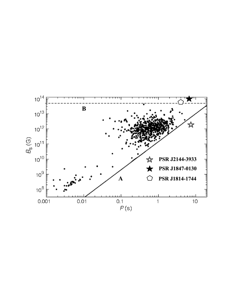
Figure 1: Line A. ”Death line” when curvature radiation with the sunspot configuration of the magnetic field is taken as the mechanism of producing the gamma quanta. Line B: $B=B_{Schw}$

Here $B_{s}=3.2\times 10^{19}\sqrt{\dot{P}P}$ is pulsar surface magnetic field inferred from observational values of spin period and period derivative, $B_{Schw}=m_{e}^{2}c^{3}/e\hbar\approx 4.4\times 10^{13}G$ is Schwinger limit i.e. the magnetic field at which the electron cyclotron energy equals the electron rest mass energy and $B_{dl}$ is the magnetic field corresponding to the so-called ”death line” (see Fig. 1) (Young et al., 1999). The various configurations of the surface magnetic field correspond to different death lines. They depend not only on magnetic field configuration, but significantly on whether the origin of gamma quanta, which are responsible for pair production, is curvature radiation or inverse Compton scattering (Zhang & Harding, 2000). As a mechanism of producing of gamma quanta we took curvature radiation with sunspot configuration of magnetic field. In this case ”death line” is defined by the condition that the potential drop across the gap required to produce enough pairs per primary to screen out the parallel electric field is larger than the maximum potential drop available from the pulsar. The quantity $B_{dl}$ can be solved from the following equation (Chen & Ruderman, 1993):

$$7\log B_{dl}-13\log P=78$$ (2)

Recently there were discovered three long period radio pulsars PSR J2144-3933 (Young et al., 1999), PSR J1847-0130 (McLaughlin et al., 2003) and PSR J1814-1744 (Camilo et al., 2000)(see Table 1), that break the condition above (the first one breaks the right-hand side of the inequality and the other two break the left). PSR J2144-3933 is distinguished by some other characteristics. It has the lowest spindown luminosity ($\dot{E}=4\pi^{2}I\dot{P}/P^{3}\approx 3.2\times 10^{28}erg\cdot s^{-1}$) of any known pulsar. The beaming fraction (that is, the fraction of the celestial sphere swept across by the beam) is also the smallest, $W\approx 1/300$. On the other hand, PSR J1847-0130 (McLaughlin et al., 2003) and PSR J1814-1744 (Camilo et al., 2000) are isolated radio pulsars having the largest, ”magnetar”-like, inferred surface dipole magnetic fields yet seen in the population: $9.4\times 10^{13}$ G and $5.5\times 10^{13}$ G, respectively. These pulsars show apparently normal radio emission in the regime of magnetic field strength ($B_{s}\geq B_{Schw}$), where plasma models predict no emission should occur. However, the nature of the Schwinger limit is not clear and is the subject of long term discussions. Baring & Harding (2001) proposed that for extremely strong fields, photon splitting dominates over pair production and the corresponding death line is a function of both field strength and period. This is definitely neither a certain nor a hard limit. Furthermore, Usov (2002) has argued that since only one photon polarization mode splits, the onset of photon splitting does not suppress the production of pairs. It is very important to investigate this interesting problem, but it is beyond the framework of our model, especially since we argue that magnetic fields of neutron stars in our investigation are less than the Schwinger limit.

A model that explains the phenomenon of radio emission from these pulsars and all their anomalous properties does not exist.

An important feature of our model, which provides a natural explanation of most of the properties of these pulsars, is the presence of very low frequency, nearly transverse drift waves propagating across the magnetic field and encircling the open field line region of the pulsar magnetosphere (Kazbegi et al., 1991b, 1996). These waves only periodically change the direction of the radio emission and are not directly observable. We give a description of this model in Sections 2, 3 and 4. Some estimates of the rotational and angular parameters of these pulsars are given in Section 5. We discuss the obtained results in Sections 6 and 7.

2 Emission model

As mentioned the pulsar magnetosphere is filled by a dense relativistic electron-positron plasma. The (e⁺e^-) pairs are generated as a consequence of the avalanche process [first described by Sturrock (1971)], and they flow along the open magnetic field lines. The plasma is multicomponent, with a one-dimensional distribution function (see Arons, 1981a, Fig.1), containing the following:

(i) electrons and positrons of the bulk of plasma with a mean Lorentz factor of $\gamma_{p}$ and density $n_{p}$;

(ii) particles of the high-energy ’tail’ of the distribution function with $\gamma_{t}$ and $n_{t}$, stretched in the direction of positive momentum;

(iii) the ultrarelativistic ($\gamma_{b}\sim 10^{6}$) beam of primary particles with so-called ’Goldreich-Julian’ density (Goldreich & Julian, 1969) $n_{b}\approx 7\times 10^{-2}B_{s}P^{-1}(R_{0}/R)^{3}\left[cm^{-3}\right]$ (where P is the pulsar period, $R_{0}\approx 10^{6}$cm is the neutron star radius, $B_{s}$ is the magnetic field value at the stellar surface and $R$ is the distance from the center of the neutron star). This density is much less than the density of secondary pairs $n_{p}$.

Let us note that such parameters are only possible under the assumption that strong and curved multipolar fields persist in the pair-production region, near the stellar surface (Arons, 1981b; Machabeli & Usov, 1989).

Such a distribution function should generate various wave-modes under certain conditions. The waves then propagate in the pair plasma of the pulsar magnetosphere, transform into vacuum electromagnetic waves as the plasma density drops, enter the interstellar medium and reach an observer as pulsar radio emission. This waves leave the magnetosphere propagating at relatively small angles to the pulsar magnetic field (Kazbegi et al., 1991a).

Particles moving along the curved magnetic field undergo drift motion transversely to the plane where the field line lies. The drift velocity can be written as

$$u=c\gamma\upsilon_{\varphi}/\omega_{B}R_{c}$$ (3)

where $\omega_{B}=eB/mc$, $B=B_{s}(R_{0}/R)^{3}$ . $R_{c}$ is the curvature radius of the dipolar magnetic field line, $\gamma$ is the relativistic Lorentz factor of a particle and $\upsilon_{\varphi}$ is the particle velocity along the magnetic field. Here and below the cylindrical coordinate system ($x,r,\varphi$) is chosen, with the $x$-axis directed transversely to the plane of the field line, while $r$ and $\varphi$ are the radial and azimuthal coordinates, respectively.

Generation of radio emission is possible if at least one of the following resonance conditions is fulfilled:

$$\quad\qquad\textrm{cyclotron instability}\qquad\omega-k_{\varphi}\upsilon_{\varphi}-k_{x}u=\frac{\omega_{B}}{\gamma_{res}}\qquad$$ (4)

$$\textrm{Cherenkov instability}\qquad\omega-k_{\varphi}\upsilon_{\varphi}-k_{x}u=0$$ (5)

These conditions are very sensitive to the parameters of the magnetospheric plasma, particularly to the value of the drift velocity (see eq.[3]), and hence to the curvature of the magnetic field lines (Kazbegi et al., 1996).

It should be noted that, in the absence of drift motion, the ordinary Cherenkov interaction implies that the phase velocity of a wave equals the velocity of the particles in both value and direction. In other words, an observer moving with the same velocity as the particles, should detect the same phase of the wave for a sufficiently long time ($\tau\sim 1/\Gamma$ ). This is, however, impossible for a wave propagating transversely to the particles’ velocity. On the other hand, the drift velocity (equation (3)) is directed along the phase velocity of such a wave. This allows wave-particle resonant interaction.

3 Generation of drift waves

It has been shown (Kazbegi et al., 1991b, 1996) that, in addition to the waves mentioned above (the characteristic frequencies of which fall into the radio band) propagating with small angles to the magnetic field lines, very low frequency, nearly transverse drift waves can be excited. They propagate across the magnetic field, so that the angle between ${\bf k}$ and ${\bf B}$ is close to $\pi/2$. In other words, $k_{\bot}/k_{\varphi}\gg 1$, where $k_{\bot}=(k_{r}^{2}+k_{\varphi}^{2})^{1/2}$ . Assuming $\gamma(\omega/\omega_{B})\ll 1$, $(u_{\alpha}/c)^{2}\ll 1$, $k_{\varphi}/k_{x}\ll 1$ and $k_{r}\rightarrow 0$, we can write the general dispersion equation of the drift waves in the following form (Kazbegi et al., 1991a, b, 1996):

$$\left(1-\sum\limits_{\alpha}\frac{\omega_{\alpha}^{2}}{\omega}\int\frac{u_{\alpha}^{2}}{\upsilon_{\varphi}c}\frac{1}{\omega-k_{\varphi}\upsilon_{\varphi}-k_{x}u_{a}}\frac{\partial f_{\alpha}}{\partial p}dp-\frac{k_{\varphi}^{2}c^{2}}{\omega^{2}}\right)\times$$

$$\left(1+\sum\limits_{\alpha}\frac{\omega_{\alpha}^{2}}{\omega}\int\frac{\upsilon_{\varphi}/c}{\omega-k_{\varphi}\upsilon_{\varphi}-k_{x}u_{a}}\frac{\partial f_{\alpha}}{\partial p}dp\frac{k_{\varphi}^{2}c^{2}}{\omega^{2}}\right)-$$

$$\left(\frac{k_{x}k_{\varphi}c^{2}}{\omega^{2}}+\sum\limits_{\alpha}\frac{\omega_{\alpha}^{2}}{\omega}\int\frac{u_{\alpha}/c}{\omega-k_{\varphi}\upsilon_{\varphi}-k_{x}u_{a}}\frac{\partial f_{\alpha}}{\partial p}dp\right)^{2}=0$$ (6)

where $\alpha$ denotes the sort of particles (electrons or positrons) and $\omega_{\alpha}^{2}=4\pi n_{\alpha}e^{2}/m$, $f_{\alpha}$ is the distribution function and $p$ is the momentum of the plasma particles.

Let us assume that

$$\omega=k_{\varphi}\upsilon_{\varphi}+k_{x}u_{b}+i\Gamma$$ (7)

where $u_{b}$ is the drift velocity of the beam particles (see eq.[3]). In the approximation $k_{\varphi}\upsilon_{\varphi}\ll k_{x}u_{b}$ and $k_{x}^{2}\ll\omega_{p}^{2}/\gamma_{p}^{3}c^{2}$, the imaginary part can be written as

$$\Gamma=Im\omega\approx\left(\frac{n_{b}}{n_{p}}\right)^{1/2}\left(\frac{\gamma_{p}^{3}}{\gamma_{b}}\right)^{1/2}k_{x}u_{b}$$ (8)

According to equation (7), the frequency of a drift wave can be written as

$$\omega_{0}=Re\omega=k_{\varphi}\upsilon_{\varphi}+k_{x}u_{b}\approx k_{x}u_{b}$$ (9)

Drift waves propagate across the magnetic field and encircle the region of the open field lines of the pulsar magnetosphere. They draw energy from the longitudinal motion of the beam particles, as in the case of the ordinary Cherenkov wave-particle interaction. However, they are excited only if $k_{x}u_{b}\neq 0$, i.e., in the presence of drift motion of the beam particles. Note that these low-frequency waves are nearly transverse, with the electric vector being directed almost along the local magnetic field. Let us note that although $k_{\varphi}\upsilon_{\varphi}\ll k_{x}u_{b}$ for the drift waves, there still exists a nonzero $k_{\varphi}$. It appears that growth rate (equation (8)) is rather small. However, the drift waves propagate nearly transversely to the magnetic field, encircling the magnetosphere, and stay in the resonance region for a substantial period of time. Although the particles give a small fraction of their energy to the waves and then leave the interaction region, they are continuously replaced by the new particles entering this region. The waves leave the resonance region considerably slower than the particles. Hence, there is no sufficient time for the inverse action of the waves on the particles. The accumulation of energy in the waves occurs without quasi-linear saturation. The amplitude of the waves grows until the nonlinear processes redistribute the energy over the spectrum. As was demonstrated by Kazbegi et al. (1991b), the strongest nonlinear process in this case is the induced scattering of waves on plasma particles. Therefore, the growth of the drift-wave amplitude continues until the decrement of the nonlinear waves $\Gamma_{NL}$ becomes equal to the linear decrement $\Gamma$. As a result, one obtains quasi-regular configurations of drift waves. Generally, the nonlinear scattering pumps the wave energy into the long-wavelength domain of the spectrum.

$$\lambda_{\max}\approx r_{LC}=\frac{cP}{2\pi}$$ (10)

Here $r_{LC}$ is the radius of the light cylinder.

According to equations (9), (10) and (3), the period of the drift waves can be written as:

$$P_{dr}=\frac{2\pi}{\omega_{dr}}=\frac{2\pi}{k_{x}u_{b}}=\frac{\lambda}{u_{b}}=\frac{e}{4\pi^{2}mc}\frac{BP^{2}}{\gamma_{b}}$$ (11)

It appears that the period of the drift wave is of the order of several seconds. It is possible to determine the relationship between $P_{dr}$, the derivative and the rate of slowing down of the neutron star from equation (11)

$$\dot{P}_{dr}=\frac{eB}{2\pi^{2}mc\gamma_{b}}P\dot{P}$$ (12)

For the considered values of the parameters we obtain $\dot{P}_{dr}\approx 10\dot{P}$ This relation is kept during the entire life of the pulsar, until it stops emitting.

4 Mechanism of field line curvature change

Let us assume that a drift wave with the dispersion defined by equation (7) is excited at some place in the pulsar magnetosphere. It follows from the Maxwell equations that $B_{r}=E_{\varphi}(k_{x}c/\omega)$, hence $B_{r}\gg E_{\varphi}$ for such a wave. Therefore, excitation of a drift wave causes particular growth of the $r$-component of the local magnetic field.

The field line curvature $\rho_{c}\equiv 1/R_{c}$ is defined in a Cartesian frame of coordinates $(x,y,z)$ (where $z$ axis is directed perpendicular to the plane of the field line) as

$$\rho_{c}=\left[1+\left(\frac{dy}{dx}\right)^{2}\right]^{-3/2}\frac{d^{2}y}{dx^{2}}$$ (13)

where $dy/dx=B_{y}/B_{x}$. Using $\left(\nabla\cdot{\bf B}\right)=0$ and rewriting equation (13) in cylindrical coordinates, we obtain

$$\rho_{c}=\frac{1}{r}\frac{B_{\varphi}}{B}-\frac{1}{r}\frac{1}{B}\frac{B_{\varphi}^{2}}{B^{2}}\frac{\partial B_{r}}{\partial\varphi}$$ (14)

Here $B=\left(B_{\varphi}^{2}+B_{r}^{2}\right)^{1/2}\approx B_{\varphi}\left[1+B_{r}^{2}/2B_{\varphi}^{2}\right]$. Assuming that $k_{\varphi}r\gg 1$, we obtain from equation (14)

$$\rho_{c}=\frac{1}{r}\left(1-k_{\varphi}r\frac{B_{r}}{B_{\varphi}}\right)$$ (15)

From equation (15) it is clear that even a small change of $B_{r}$ causes a significant change of $\rho_{c}$. The variation of the field line curvature can be estimated as

$$\frac{\Delta\rho_{c}}{\rho_{c}}\approx k_{\varphi}r\frac{\Delta B_{r}}{B_{\varphi}}$$ (16)

It follows that even a drift wave with a modest amplitude $B_{r}\sim\Delta B_{r}\sim 0.01B_{\varphi}$ alters the field line curvature substantially, $\Delta\rho_{c}/\rho_{c}\sim 0.1$

Since radio waves propagates along the local magnetic field lines, curvature variation causes a change of the emission direction.

5 The model

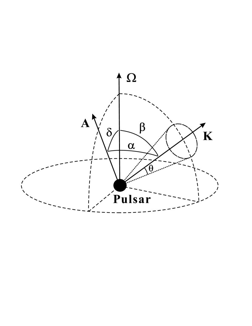
Figure 2: Geometry of rotation ($\Omega$), emission (K), and observers (A) axes. Angles $\delta$ and $\vartheta$ are constants, while $\beta$ and $\alpha$ are oscillating with time.

There is unequivocal correspondence between the observable intensity and $\alpha$ (the angle between the observer’s line of sight and the emission direction (see Fig. 2)). The maximum of the intensity corresponds to the minimum of $\alpha$. The period of a pulsar is the time interval between the neighboring maximums of the observable intensity (minimums of $\alpha$). According to this fact, we can say that the observable period is representative of the value of $\alpha$ and as it appears below, it might differ from the spin period of the pulsar.

$$\cos\alpha={\bf A}\cdot{\bf K}$$ (17)

where ${\bf A}$ and ${\bf K}$ are unit guide vectors of observer’s and emission axes, respectively. In the spherical coordinate system ($r,\varphi,\theta$), combined with the plane of the pulsar rotation, these vectors can be expressed as:

$${\bf A}=\left(1,0,\delta\right)$$ (18)

$${\bf K}=\left(1,\Omega t,\beta\right)$$ (19)

where $\Omega=2\pi/P$ is the angular velocity of the pulsar. $\delta$ is the angle between the rotation and observer’s axes, and $\beta$ is the angle between the rotation and emission axes (see Fig. 2).

From equations (17),(18) and (19), it follows that:

$$\alpha=\arccos\left(\sin\delta\sin\beta\cos\Omega t+\cos\delta\cos\beta\right)$$ (20)

In the absence of the drift wave $\beta=\beta_{0}=const$, and consequently the period of $\alpha$ is equal to $2\pi/\Omega$.

According to equation (16), in the presence of the drift wave, the fractional variation $\Delta\rho_{c}/\rho_{c}$ is proportional to the magnetic field of the wave $B_{r}$, which is periodically changing. So $\beta=\beta\left(t\right)$ is harmonically oscillating about $\beta_{0}$ with an amplitude $\Delta\beta=\Delta\rho_{c}/\rho_{c}$ and rate $\omega_{dr}=2\pi/P_{dr}$ . Thus, we can write that

$$\beta=\beta_{0}+\Delta\beta\sin\left(\omega_{dr}t+\varphi\right)$$ (21)

According to equations (20) and (21,) we obtain

$$\alpha=\arccos\left(\sin\delta\sin\left(\beta_{0}+\Delta\beta\sin\left(\omega_{dr}t+\varphi\right)\right)\cos\Omega t+\cos\delta\cos\left(\beta_{0}+\Delta\beta\sin\left(\omega_{dr}t+\varphi\right)\right)\right)$$ (22)

$$\alpha_{\min}^{k}=\left|\left(\beta_{0}-\delta\right)+\Delta\beta\sin\left(2\pi k\frac{\omega_{dr}}{\Omega}+\varphi\right)\right|$$ (23)

$\alpha_{\min}^{k}$ is the minimum of $\alpha$ after $k$ revolutions of the pulsar . The parameters of the pulse profile (e.g. width, height etc.) significantly depend on what the minimal angle would be between the emission axis and the observer’s axis while first one passes the other (during one revolution). If the emission cone does not cross the observer’s line of sight entirely (i.e., the minimal angle between them is more than cone angle $\vartheta$, see inequality (24a)), then we cannot observe the pulsar emission. On the other hand, inequality (24b) defines condition that is necessary for emission detection.

$$\alpha_{\min}^{k}>\vartheta$$ (24a)

$$\alpha_{\min}^{k}<\vartheta$$ (24b)

Hence, for some values of parameters $\Omega$, $\omega_{dr}$, $\beta$, $\Delta\beta$, $\delta$, $\varphi$ and $\vartheta$ (Set A) it is possible to accomplish the following regime: after every $k=m$ turn, the minimal value of $\alpha$ ($\alpha_{\min}^{m}$ ) satisfies condition (24b) while for intervening values of $k$ ($1\leq k\leq(m-1)$, where $k$ and $m$ are positive integers), $\alpha_{\min}^{m}$ satisfies condition (24a). In that case the observable period $P_{obs}$ does not represent the real pulsar spin period, but is divisible by it.

$$P_{obs}=mP$$ (25)

Hence,

$$\dot{P}_{obs}=m\dot{P},$$ (26)

where $P$ is the pulsar spin period.

The dipolar magnetic field strength on the neutron star surface can be written as:

$$B=3.2\times 10^{19}\sqrt{\dot{P}P}$$ (27)

From equations (25),(26) and (27), it follows that

$$B=\frac{B_{obs}}{m}$$ (28)

After inserting equations (28) and (25) in equation (2), we obtain:

$$7\log B-13\log P=(7\log B_{obs}-13\log P_{obs})+6\log m\geq 78$$ (29)

Then

$$6\log m\geq 78-7\log B_{obs}+13\log P_{obs}$$ (30)

It can be verified that there exists value for $m$ that satisfies equation (30) and the following condition simultaneously

$$B=\frac{B_{obs}}{m}<B_{Schw}$$ (31)

Thus, it is possible to fulfil the conditions necessary for $($e⁺e${}^{-})$ pair production for some values of $m$.

There is a common problem for pulsars II and III presented in Table 1 (their surface magnetic field strength exceeds the quantum critical value $B>B_{Schw}$), whereas for PSR J2144-3933 the problem appears in a different way. Equation (29) is not fulfilled. After substituting $B_{obs}$ and $P_{obs}$ from Table 1 in equation (30), we obtain:

$$6\log m\geq 4$$ (32)

Thus, if equation (32) is accomplished, it is possible for PSR J2144-3933 to generate radio emission.

For better estimation of $m$ we can use observational data for beaming fractions. From Figure 2 appears that the pulse width can be expressed as:

$$W=P\times 2\sin\theta/2\pi\sin\delta,$$ (33)

after inserting equation (25) in equation (33), we obtain:

$$mW/P_{obs}=\sin\theta/\pi\sin\delta$$ (34)

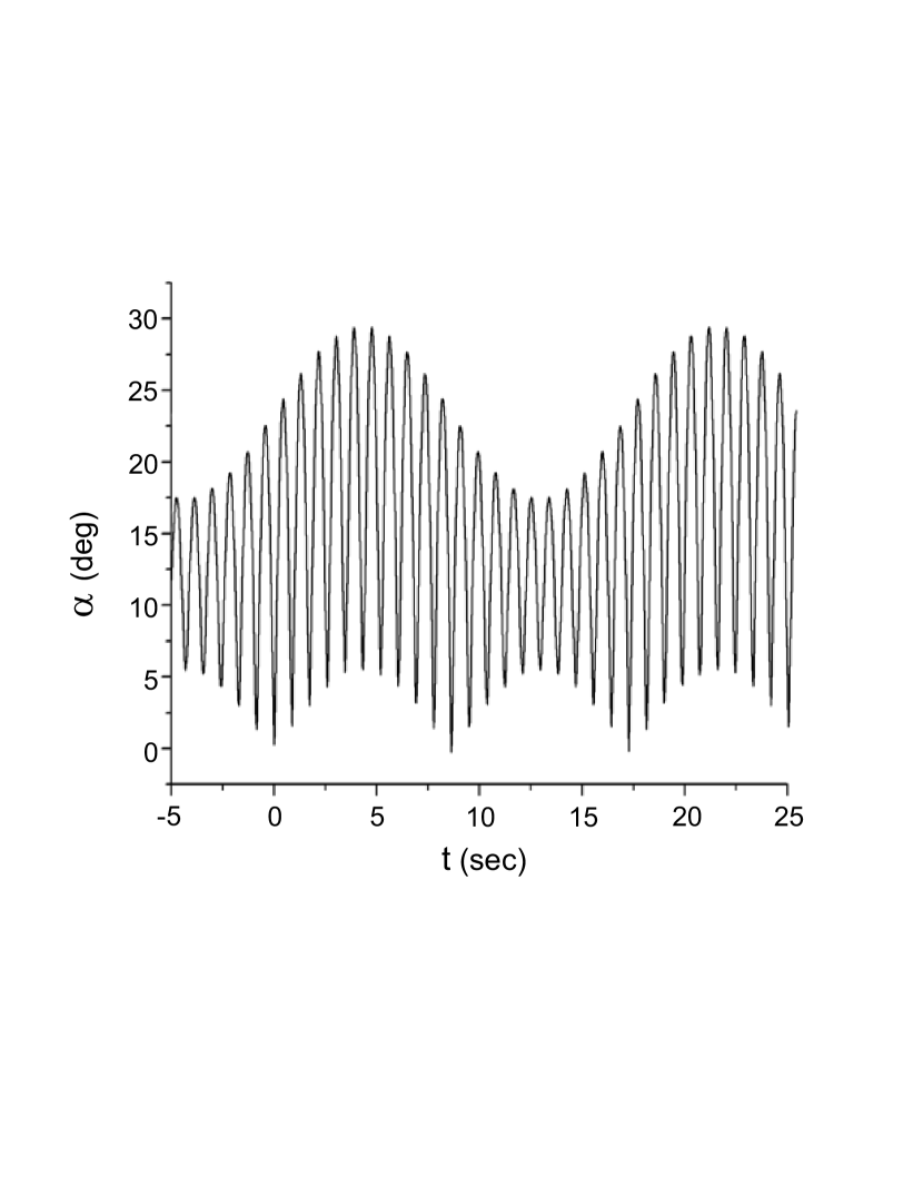
Figure 3: Oscillating behavior of $\alpha$ with time for $\beta_{0}=\delta\approx 0.12$, $\Delta\beta=0.12$, $\omega_{dr}=2\pi/17(s^{-1})$, $\Omega=2\pi/0.85(s^{-1})$, $\varphi=0$; $t_{1}=2\pi/\Omega$, $t_{2}=4\pi/\Omega$

As was mentioned above, to accomplish the described regime (eq.[25]), (the angle between the observer’s line of sight and the emission direction after one revolution from that moment when they were coincident ($\alpha=0$, Fig. 3)) $\alpha_{\min}^{m}$ must exceed $\theta$. Since

$$\alpha_{min}^{1}=\Delta\beta(2\pi P/P_{dr}),$$ (35)

if we assume that $\beta_{0}=\delta$, then we get $P_{dr}=2P_{obs}=2mP$ and

$$\theta_{max}=\Delta\beta(\sin\pi/m);$$ (36)

if we substitute this equation in equation (34), we obtain:

$$W/P_{obs}=\Delta\beta(\sin\pi/m)/m\pi\sin\delta$$ (37)

Here the left-hand side is known from the observations. Equation (37) gives us the ability to estimate the angular parameters of pulsars for the given values of $m$.

If we consider these pulsars in the framework of our model, their parameters (e.g. spin and angular parameters) will get new ’real’ values, shown in Table 2.

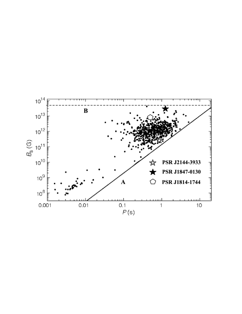
Figure 4: $(P-B_{s})$ diagram of the real positions of the considered pulsars, corresponding to Table 2.

According to the obtained results, the considered pulsars are placed on (P-B) diagram as shown in Fig. 4

Thus, we developed the theoretical model of pulsar emission, in the framework of which we explained all specific features of pulsars presented in Table 1.

6 Discussion

It should be noted that this model is applicable to the entire population of pulsars, but the effects caused by drift waves are different depending on the values of the parameters (Set A). In the case of large $\Delta\beta$ ($\Delta\beta>\vartheta$), the most interesting effect is the lengthening of the observable period (see eq.[25]) which is accomplished only when $P_{dr}$ is divisible by $P$ to high accuracy. It explains the lack of such kinds of pulsars.

In the case of small $\Delta\beta$ ($\Delta\beta<\vartheta$), the observable period does not increase (except for $\left|\beta_{0}-\delta\right|\approx\Delta\beta$ ), but some other interesting effects appear, such as drifting subpulses (Kazbegi et al., 1991c) and period and period derivative oscillation phenomenon, which is observed in PSR B1828-11 (Stairs et al., 2000) and PSR B1642-03 (Shabanova et al., 2001). Some authors (Jones & Andersson, 2001; Link & Epstein, 2001; Rezania, 2003) have proposed different models to explain this phenomenon within the framework of free precession of the neutron star. As shown by Shaham (1977) and Sedrakian et al. (1999) the existence of precession in the neutron star is in strong conflict with the superfluid models for the neutron star interior structure. Therefore, we can declare that there does not yet exist a self-consistent explanation of this fact. We plan to study this problem in detail in a forthcoming paper.

If $P_{dr}$ is not divisible by $P$, then the observed intensity must be modulated with the period of the drift wave. It is impossible to get such variations with integrated pulse profiles. Deviations of integrable pulse intensities damp each other. The only possible way to prove this scenario is by single pulse observations. Such observations really show intensity variations (Karastergiou et al., 2001). Although they do not have have a harmonic nature (this is due to various noises and insufficient resolution), it benefits our model. So if experiments are modified to evolve the oscillating component, it would help validate our theory.

Let us consider pulsars with very short periods. As mentioned above, drift waves arise in the vicinity of the light cylinder. The shorter the pulsar spin period, the smaller is the radius of the light cylinder, and consequently. the larger is the magnetic field value in the wave generation region ($B_{\varphi}\approx B=B_{s}(R_{0}/R)^{3}$). Thus, if we take this consideration into account, from equation (16) it follows that for pulsars whose period is much less than $0.1s$, the amplitude of the oscillation in the emission direction would be so small ($\Delta\beta<1^{o}$), that the presence of drift waves would not cause any significant effect.

We believe that if the scenario defined above (enlarging of the observable period due to emission direction changing by drift waves) is accomplished then there must be simultaneous modulation of the radio and X-ray emission. Some evidence of this fact is detected radio emission from SGR 1900+14 (Shitov, 1999) and AXP 1E2259+586 (Malofeev & Malov, 2001). Higher radio frequency emission from these magnetars has not been observed yet, but discussion about this issue differs from objectives of our paper. However, detection of both types of emission is rare event, because they are generated on different altitudes, radio and X-ray emission propagate in different directions. This implies that the pulsars considered in this paper do not show X-ray emission.

7 Conclusions

After these considerations we can divide radio pulsars into the following groups, which are listed with their main requirements:

1. Rapidly rotating pulsars, for which $\Delta\beta$ is too small. None of the mentioned effects there should exist for these.

2. Pulsars with $\Delta\beta<\vartheta$ and $(P_{dr}-P)/P_{dr}<<1$. In this case, period, period derivative and pulse shape oscillation should appear. In the case of low accuracy of equality between $P_{dr}$ and $P$, subpulse drift can be observed (Kazbegi et al., 1991a; Gogoberidze et al., 2005).

3. Pulsars with $\Delta\beta<\vartheta$. They should show observed intensity variations, modulated with the period of the drift waves.

4. Pulsars with $\Delta\beta>\vartheta$ and ${(P_{dr}-mP)/P}<<1$ (where $m$ is a positive integer). These appear different from the real, long observable rotation period.

Thus, long-period radio pulsars represent one of the branches of usual pulsars and must be considered in the frameworks of traditional theories for the specific values of the parameters (Set A).

Table 1: Radio pulsars with long periods.

No	Pulsar	$P(s)$	$\dot{P}(10^{-15}s\cdot s^{-1})$	$B_{s}(10^{12}G)$	$\dot{E}(10^{32}erg\cdot s^{-1})$
I	PSR J2144-3933	8.5	0.48	2	0.00032
II	PSR J1847-0130	6.7	1275	94	1.7
III	PSR J1814-1744	4.0	743	55	4.7

Table 2: The ’real’ values of pulsar parameters.

Pulsar	$m$	$P_{dr}$	$P$	$\dot{P}$	$B_{s}$	$\dot{E}$	$\Delta\beta$	$\beta_{0}\approx\delta$	$\vartheta$	$W_{10}/P$
		(s)	(s)	$(10^{-15}s\cdot s^{-1})$	$(10^{12}G)$	$(10^{32}erg\cdot s^{-1})$	(deg)	(deg)	(deg)
PSR J2144-3933	10	17.0	0.85	0.048	0.2	0.032	$7^{o}$	$7^{o}$	$1.5^{o}$	0.1
PSR J1847-0130	6	13.4	1.12	210	16	61	$5^{o}$	$5^{o}$	$3^{o}$	0.3
PSR J1814-1744	8	8.0	0.5	93	6.9	300	$5^{o}$	$5^{o}$	$2^{o}$	0.2

References

- Arons (1981a) Arons J., 1981a, in Plasma Astrophys. ed. T.D.Guyenne and G.Levy (ESA SP-161, Paris: ESA), 273
- Arons (1981b) Arons J., 1981b, ApJ, 248, 1099
- Baring & Harding (2001) Baring M.G., & Harding A.K., 2001, ApJ, 547, 929
- Camilo et al. (2000) Camilo, F., et al. 2000, ApJ, 541, 367
- Chen & Ruderman (1993) Chen, K., & Ruderman, M. A. 1993, ApJ, 402, 264
- Gogoberidze et al. (2005) Gogoberidze, G., Machabeli, G.Z., Melrose, D.B. & Luo, Q. 2005, MNRAS, 360, 669
- Goldreich & Julian (1969) Goldreich P., Julian H., 1969, ApJ, 157, 869
- Jones & Andersson (2001) Jones, D. I., & Andersson, N. 2001, MNRAS, 324, 811
- Karastergiou et al. (2001) Karastergiou, A., von Hoensbroech, A., Kramer, M., Lorimer, D. R., Lyne, A. G., Doroshenko, O., Jessner, A., Jordan, C., Wielebinski, R. 2001, A&A, 379, 270
- Kazbegi et al. (1991a) Kazbegi A. Z., Machabeli G. Z., Melikidze G. I., 1991a, MNRAS, 253, 377
- Kazbegi et al. (1991b) Kazbegi A. Z., Machabeli G. Z., Melikidze G. I., 1991b, Austral. J. Phys., 44, 573
- Kazbegi et al. (1991c) Kazbegi A. Z., Machabeli G. Z., Melikidze G. I., Smirnova T. V., 1991c, Afz, 34, 433
- Kazbegi et al. (1996) Kazbegi A. Z., Machabeli G. Z., Melikidze G. I., Shukre C., 1996, A&A, 309, 515
- Link & Epstein (2001) Link, B., & Epstein, R. I. 2001, ApJ, 556, 392
- Machabeli & Usov (1989) Machabeli G. Z., Usov V. V., 1989, Sov. Astron. Letters, 15, 393
- Malofeev & Malov (2001) Malofeev V.M., Malov O.I. 2001, in Physics of Neutron Stars, ed. D.A.Varshalovich et al. (St. Petersburg Ioffe Physical Technical Institute), 37
- McLaughlin et al. (2003) McLaughlin M.A., Stairs J.H., Kaspi V.M. et al. 2003, ApJ, 591, L135
- Rezania (2003) Rezania, V. 2003, A&A 399, 653
- Sedrakian et al. (1999) Sedrakian, A., Wasserman, I., & Cordes, J. M. 1999, ApJ, 524, 341
- Shabanova et al. (2001) Shabanova, T. V., Lyne, A. G., & Urama, J. O. 2001, ApJ, 552, 321
- Shaham (1977) Shaham, J. 1977, ApJ, 214, 251
- Shitov (1999) Shitov, Yu.P. 1999, IAU Circ. 7110
- Stairs et al. (2000) Stairs, I. H., Lyne, A. G., & Shemar, S. 2000, Nature, 406, 484
- Sturrock (1971) Sturrock P. A., 1971, ApJ, 164, 529
- Usov (2002) Usov V. V., 2002, ApJ, 572, 87
- Young et al. (1999) Young M. D., Manchester R. N., & Johnston S. 1999, Nature, 400, 848.
- Zhang & Harding (2000) Zhang, B., & Harding, A. K. 2000, ApJ, 535, L51