Smoothing Algorithms and High-order Singularities in Gravitational Lensing

Abstract

We propose a new smoothing method for obtaining surface densities from discrete particle positions from numerical simulations. This is an essential step for many applications in gravitational lensing. This method is based on the “scatter” interpretation of the discrete density field in the Smoothed Particle Hydrodynamics. We use Monte Carlo simulations of uniform density fields and one isothermal ellipsoid to empirically derive the noise properties, and best smoothing parameters (such as the number of nearest neighbors used). A cluster from high-resolution simulations is then used to assess the reality of high-order singularities such as swallowtails and butterflies in caustics, which are important for the interpretation of substructures in gravitational lenses. We also compare our method with the Delaunay tesselation field estimator using the galaxy studied by Bradac et al. (2004), and find good agreements. We show that higher order singularities are not only connected with bound subhaloes but also with the satellite streams. However, the presence of high-order singularities are sensitive to not only the fluctuation amplitude of the surface density, but also the detailed form of the underlying smooth lensing potential (such as ellipticity and external shear).

1 INTRODUCTION

Gravitational lensing provides an important technique to study the matter distribution in the universe (e.g., Kochanek, Schneider & Wambsganss 2004). On galaxy-scales, simple smooth isothermal models appear to match the gravitational lenses reasonably well (e.g., Kochanek 1991), although there are some difficulties in accurately reproducing the observed flux ratios. At present, it is unclear what causes these “anomalous flux ratios” (e.g., Kochanek & Dalal 2005; Mao et al. 2004; Macciò et al. 2006; Macciò & Miranda 2006). On cluster scales, it became clear early on that smooth spherical models under-predict the number of giant arcs by orders of magnitude (e.g., Bartelmann & Weiss 1994; Bartelmann et al. 1995; Bartelmann et al. 1998). Ellipticity and substructures in clusters have dramatic effects on the lensing cross-sections of giant arcs. This is because many massive clusters are more or less super-critical, so a small change in the surface density or the shear can have a large nonlinear effect on the lensing properties.

The effects of ellipticity and substructures are difficult to model analytically. The most realistic way to account for these is to use numerical simulations. $N$-body simulations can accurately track the evolution of dark matter particles to highly non-linear regimes. State-of-the-art simulations can resolve dark matter haloes with several million (or more) particles within the virial radius. Even at such high resolutions, each particle in the simulation is only a Monte Carlo realization of the underlying (smooth) density field. To predict the lensing properties of the discrete particle distributions, the first step is to obtain an accurate smoothed surface density field. The fluctuations of the smoothed surface density maps directly affect the shapes, magnifications and orientations of images, and as a consequence, the lensing cross-sections and optical depths. In addition, high-resolution $N$-body simulations indicate that there are also many substructures in galaxies and clusters of galaxies. A good smoothing algorithm must be able to obtain a surface density map with sufficiently low noise level while retaining the information of substructures.

Previous workers have proposed many different algorithms for smoothing. Bartelmann et al. (1998, hereafter B98) used a three-dimensional Gaussian kernel to calculate the density on a three-dimensional grid and then integrate along the line of sight to obtain the surface density. Bradac al. (2002) directly obtained the surface density using a Gaussian kernel with a fixed smoothing length on the projected particle distributions. Li et al. (2005) and Macciò et al. (2006) used adaptive kernels commonly used in the Smoothed Particle Hydrodynamics (SPH) with similar numbers of neighbors to obtain the surface density. The most complex method was used by Bradac et al. (2004) who obtained the volume density using the Delaunay tessellation field estimator (Schaap & van de Weygaert 2000). and then projected the 3D density onto a 2D grid. Other methods can also operate on a 2D particle distribution with simple smoothing kernels, such as the nearest grid points, cloud-in-cell, and triangular shaped clouds (see Bartelmann 2003 for a review).

It is straightforward to show that for smoothing kernels (such as Gaussian kernels) with a fixed smoothing length, the same results are obtained if one directly smoothes the 2D projected particle distribution or if one first obtains the three-dimensional density distribution and then performs the projection. Furthermore, the noise levels from these two methods are identical. Therefore, if one uses smoothing kernels with a fixed length, there is no need to perform the smoothing in 3D, one can simply perform the smoothing on the projected particle distributions, saving both memory and CPU time. Of course, the particles in the $N$-body simulations are not really infinitesimal points, they in fact represent Monte Carlo realizations of a small but finite volume in the phase space. The volume a particle occupies is inversely proportional to the local mass density: in high density regions, the particles occupy a smaller volume and vice versa. Adaptive smoothing is therefore essential to account for the large variation in the local densities.

In general, the noise level is higher if one first projects the particle positions to 2D and then smoothes the density rather than first smoothing the density in 3D and then performing the projection. This is because in the first method, when we use adaptive smoothing (e.g., for a fixed number of neighbors in SPH), there is an extra noise contribution due to chance alignments. This effect is particularly serious for low-density regions. In addition, substructures will be more difficult to identify in the projected particle distributions. It is therefore important to adaptively smooth the density field in 3D and perform the projection afterwards, in order to reduce the noise level and retain the substructures. The Delaunay tessellation field estimator used by Bradac et al. (2004) is a significant step, but the method, as the authors pointed out, is quite time-consuming. To improve the computational efficiency, Ascalibar & Binney (2004) proposed a new method, FiEstAS, which can calculate the phase-space density distribution (in 6D) efficiently. However, in this method, there is some ambiguity about the smoothing length and kernel. In this paper, we concentrate on the SPH smoothing in 3D, and show that it can be used to obtain low-noise surface density maps while at the same time retaining the substructures. In §2, we discuss our method. In §3, we study the noise properties of the method for a uniform density field and an isothermal ellipsoid; analyses of noise properties for these simple cases have not yet been performed in great detail in the literature (see Lombardi & Schneider for a general discussion). We then take a cluster from cosmological simulations of structure formation, and study the reality of high-order singularities, and how they are connected with substructures and satellite streams. As shown by Bradac et al. (2004), these tend to produce large flux anomalies compared with simple analytical predictions, so it is crucial to check what produced these and whether they are real and not from numerical noise. For this purpose, we also present a detailed comparison between our method and the Delaunay tessellation method (Schaap & van de Weygaert 2000) used by Bradac et al. (2004) for their simulated galaxy. In §4, we discuss the implications of our results on the detections of substructures in lensing galaxies and clusters.

2 METHOD

The central idea of the new smoothing algorithm is to use the three-dimensional density field information, but smooth the density in two-dimensions with SPH kernels. (Our method also applies to Gaussian smoothing kernels, as long as we choose the smoothing length accordingly.) Specifically, we first choose the smoothing length according to the number of neighbors (${N_{\rm ngb}}$) in 3D. The SPH smoothing kernel is given by

$$W(r)={\sigma\over h^{\nu}}\left\{\begin{array}[]{ll}1-{3\over 2}({r\over h})^{2}+{3\over 4}({r\over h})^{3}&\mbox{for}\quad 0\leq{r\over h}\leq 1\\ {1\over 4}{(2-{r\over h})}^{3}&\mbox{for}\quad 1<{r\over h}\leq 2\\ 0&\mbox{otherwise}\end{array}\right.\;,$$ (1)

where $\nu$ is the number of dimensions, $\sigma$ is a normalization with the values: $2/3$, $10/7\pi$, $1/\pi$ in one, two and three dimensions respectively, and $2h$ is the radius of a sphere (or a circle in 2D and half-length in 1D) which contain all the neighbours. This method is fully adaptive: for high-density regions, the smoothing length will be smaller and vice versa. Once the smoothing length is determined, we distribute the particle mass onto the surrounding grid points. The weights are derived from the SPH kernel in two dimensions, using the particle’s smoothing length and its distance from the grid point in the projection plane. This corresponds to the “scatter” method in calculating the density in SPH, see Hernquist & Katz (1989). The smoothed surface density on a grid point along any projection can then be obtained by simply adding up the contributions of all the grid points that have non-vanishing contributions. We refer our method as the “scatter and integrate” (SI) method. This method uses three-dimensional density information, but as the partition of the particle weight onto the grid points is performed only once, it can be implemented efficiently.

3 RESULTS

In the following, we will apply our method and examine its performance in three cases. 1) a uniform density field, in order to understand the noise property of this method; 2) an isothermal ellipsoid; in this case, we will examine how different smoothing methods reproduce the well-known analytical critical curves and caustics. We will also check whether noise can produce high-order singularities such as swallowtails. 3) A simulated galaxy cluster taken from Jing & Suto (2002). For this cluster, we will check how well the (sub)structures are preserved in the smoothed surface density maps, and how they affect high-order singularities and the cusp relation in different smoothing methods in §3.3. In §3.4, we make detailed comparisons of our method with the Delaunay tessellation method for the simulated galaxy used by Bradac et al. (2004).

3.1 Uniform density field

We randomly generate ${N_{\rm p}}$ point particles in a cube with a unit sidelength. We use ${N_{\rm p}}=6000,48000,384000$, and 3072000; they roughly span the range found from low-resolution to high-resolution simulated clusters within the virial radius. For each simulated cube, we then obtain the volume density $\hat{\rho}$ at 4000 random positions in 3D using the SPH kernel with ${N_{\rm ngb}}=32,128,256,512$, and the surface density $\hat{\kappa}$ on a $50\times 50$ grid using the SI method we discussed above and the standard 2D SPH smoothing with the same number of neighbors, ${N_{\rm ngb}}$. Obviously both the volume and surface densities have an expectation value of unity, $\bar{\rho}=1$ and $\bar{\kappa}=1$.

The left panel in Fig. 1 shows the noise behavior for the volume density. The standard deviation of the volume density can be well fitted as

$${\sigma_{\rho}\over\bar{\rho}}\approx{2\over\sqrt{{N_{\rm ngb}}}}.$$ (2)

If we smooth the density field using SPH kernels directly in the projected particle distribution, we find that

$${\sigma_{\kappa}\over\bar{\kappa}}={1.698\over\sqrt{{N_{\rm ngb}}}}\approx\sqrt{{2\over 3}}~{}~{}{\sigma_{\rho}\over\bar{\rho}}$$ (3)

The factor $\sqrt{2/3}$ arises because the noise contribution along the line of sight has been eliminated due to integration.

If we use the scatter and integrate (SI) method discussed above, we find that the noise scales as

$$\left({\sigma_{\kappa}\over\bar{\kappa}}\right)_{\rm SI}={1.627\over{N_{\rm ngb}}^{1/3}{N_{\rm p}}^{1/6}}$$ (4)

This fitting formula matches the noise properties in our simulations quite well, as can be seen in Fig. 1.

It may appear that eqs. (3) and (4) are very different. In fact, for the same fixed smoothing length, these two formulae are related. In the following arguments, to avoid confusion, we label the number of neighbor in 2D and 3D explicitly. For an $N_{\rm ngb3d}$ neighbor in 3D, the smoothing length scales as $r_{\rm s}\propto{N_{\rm ngb3d}}^{1/3}{N_{\rm p}}^{-1/3}$. The number of neighbors in 2D will be $N_{\rm ngb2d}\propto r_{\rm s}^{2}{N_{\rm p}}\propto{N_{\rm ngb3d}}^{2/3}{N_{\rm p}}^{1/3}$. Putting this into eq. (3) yields $\sigma_{\kappa}/\bar{\kappa}\propto{N_{\rm ngb3d}}^{-1/3}{N_{\rm p}}^{-1/6}$, identical to the dependence on ${N_{\rm p}}$ and ${N_{\rm ngb}}$ as given in eq. (4). For a non-uniform field, however, our method will yield a more exact local density since the chance alignments due to projections are eliminated and, more importantly, the information of substructures and voids is better kept. We will illustrate these in §3.4.

3.2 Isothermal ellipsoids

Isothermal ellipsoids (e.g., Kormann, Schneider & Bartelmann 1994; Keeton & Kochanek 1998) are reasonable models for galaxy-scale lenses. They have analytical critical curves and caustics, so they offer an ideal model to test and calibrate different smoothing algorithms.

We generated many realizations of an oblate isothermal cluster. Its physical density is given by (cf. eq. 2 in Keeton & Kochanek 1998)

$$\rho={{v_{\rm c}}^{2}\over 4\pi Gq_{3}}{e\over\sin^{-1}e}{1\over s^{2}+R^{2}+z^{2}/q_{3}^{2}},$$ (5)

where $v_{\rm c}$ is the circular velocity of the halo, $s$ is the core radius, $q_{3}$ is the ratio of the minor axis to the other two equally long axes, and $e=\sqrt{1-q_{3}^{2}}$. We take $v_{\rm c}$ to be 1500 $\,\rm km\,{s}^{-1}$, $s=20$ kpc, and $q_{3}=0.5$. The cluster is viewed along one of the two major axes, resulting in elliptical isophotes with an axial ratio of 0.5. We generate particles within a cube of sidelength of $4\,\rm Mpc$. Below we present the results from two realizations. The low-resolution simulation has a total of ${N_{\rm p}}=54760$ particles in the box, each with mass ${M_{\rm p}}=1.6\times 10^{10}h^{-1}M_{\odot}$, while the high-resolution simulation has ${M_{\rm p}}=0.05\times 10^{10}h^{-1}M_{\odot}$ and ${N_{\rm p}}=1748982$. Here, $h$ is the Hubble constant in units of $100\,\rm km\,{s}^{-1}\,\rm Mpc^{-1}$. They roughly span low-resolution and high-resolution clusters typically found in numerical simulations. The redshift of the lens and source are taken to be 0.3 and 1.0 respectively, and we assume the $\Lambda$CDM cosmological model (see §3.3).

Different $\kappa$ maps on a 2048$\times$ 2048 grid are produced by the 2D SPH and SI method for these two Monte-Carlo simulations. The lensing potential is then obtained using the fast Fourier transform method (Bartelmann et al. 1998). To resolve the critical curves well, we perform cubic spline interpolations of the lensing potential on a finer grid (Li et al. 2005). At the same time, we derive the magnification and the lens mapping from the image plane to the source plane on the whole grid. To locate the critical curves, we use the fact that they separate regions of different signs of magnifications in the image plane (see, e.g., Bartelmann 2003 for a practical implementation).

Fig. 2 shows the surface density obtained for the low-resolution simulation for different smoothing algorithms and parameters together with the predicted analytical surface density. The surface density is plotted as a function of the ellipsoidal radius. As can be seen, the analytical surface density is reproduced quite well by both the 2D SPH and the SI method, except in the inner-most regions where the numerical results are lower due to smoothing.

The noise in the surface density is obtained from the fluctuations in the surface density of all pixels within each elliptical annulus. For the 2D SPH smoothing, this is a function of the number of neighbors only, and is independent of ${N_{\rm p}}$ or the distribution of the surface density. Eq. (3) appears to match the noise in the data quite well (see the top panels in Fig. 2). On the other hand, for the SI method, the surface density is obtained by an integration of the volume density along the line of sight. While the relative error of the volume density only depends on the number of neighbors used, the absolute error depends on the local density through the integration along the line of sight. From the lower panels in Fig. 2, we see that the noise level changes with radius, but it appears that eq. (4) still provides a reasonable approximation to the errors except in the innermost regions. However, the noise in $N$-body simulations is not completely Poissonian because the particles follow dynamical evolution and their phases are correlated. Studies about the errors in $N$-body simulations (Monaghan 1992; Niedereiter 1978) show that they are generally smaller than a naive estimate from pure Poissonian noise. Nevertheless, we believe our empirical formula eq. (4) still provides an approximate measure of the noise in the surface density from cosmological $N$-body simulations.

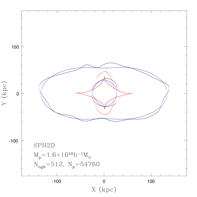
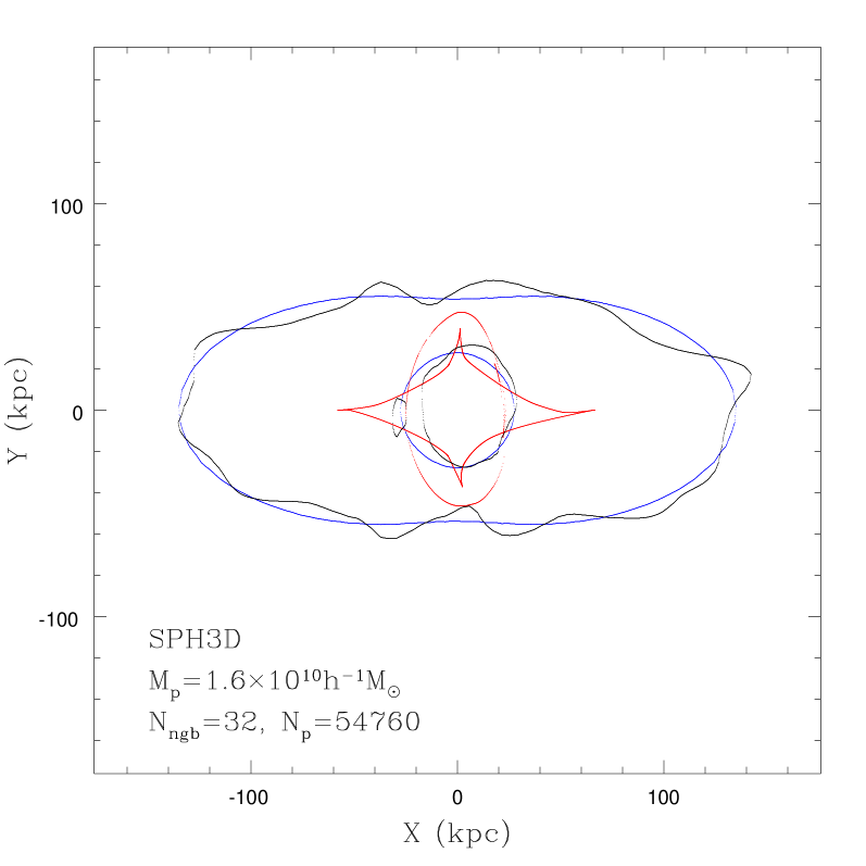
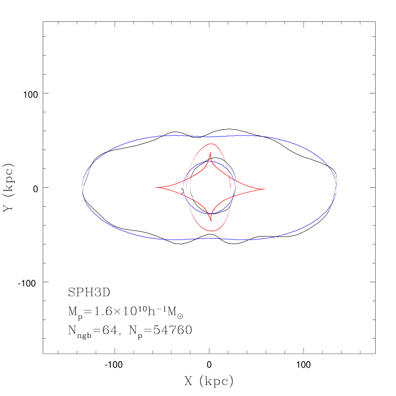
Figure 3: The caustics and critical curves in the SI method and the 2D SPH smoothing method. The particle mass and the particle number used to smooth are indicated for each. The blue lines are the analytic critical curves, the black and red lines are the critical curves and caustics obtained from the Monte Carlo simulations.

Fig. 3 shows the resulting critical curves and caustics for the smoothed density field of the low resolution realization. It is clear that for the 2D SPH smoothing, when ${N_{\rm ngb}}=128$, the critical curves show large deviations from the analytical results, and the caustics show a large number of high-order singularities, such as swallowtails and butterflies. The agreement is substantially better when ${N_{\rm ngb}}$ is increased to 512 in the 2D SPH smoothing, in this case all the prominent higher-order singularities disappear (in agreement with analytical predictions). This demonstrates that these are due to artifacts of inappropriate smoothing. For the SI method, with ${N_{\rm ngb}}=32$, the critical curves and caustics already resemble the analytical results quite well, with no apparent high-order singularities. Increasing ${N_{\rm ngb}}$ by a factor of 2 does not change the critical curves and caustics substantially.

The results are similar for the high-resolution Monte Carlo simulation. Compared with the lower resolution, the surface density (Fig. 4) is reproduced well even in the inner-most regions due to the increased particle number. Again the 2D SPH smoothing algorithm appears to produce artificial high-order singularities (see Fig. 5) for ${N_{\rm ngb}}=128$; some remain even for ${N_{\rm ngb}}=512$. In contrast, the SI method does not produce prominent higher-order singularities.

The SI method is also computationally efficient. For the low resolution cluster, the speed for the SI method is similar to that for the 2D SPH smoothing method. But for the high resolution simulation, for the same noise level, the SI method is much faster, as the 2D SPH smoothing algorithm requires many more neighbors to be taken into account.

3.3 A cluster from numerical simulations and its high-order singularities

As we mentioned before, the fluctuations in the Monte Carlo simulations discussed above for the uniform density field and the isothermal ellipsoid arise due to Poisson statistics. In $N$-body simulations, the noise may be significantly smaller than the Poisson noise. Furthermore, substructures cannot be properly accounted for in our simple simulations. To remedy this, we study a numerically simulated cluster.

3.3.1 Numerical simulations, substructures and streams

The cosmological model considered here is the current popular $\Lambda$CDM model with the matter-density parameter $\Omega_{0}=0.3$ and the cosmological constant $\Lambda_{0}=0.7$ ($\Lambda$CDM). The shape parameter $\Gamma=\Omega_{0}h$ and the amplitude $\sigma_{8}$ of the linear density power spectrum are taken to be 0.21 and 0.9, respectively, where $h=0.7$ is again the Hubble constant in units of $100\,\rm km\,{s}^{-1}\,\rm Mpc^{-1}$. A cosmological $N$-body simulation with a box size $L=100h^{-1}\,\rm Mpc$, which was generated with a vectorized-parallel $\,\rm P^{3}M$ code (Jing & Suto 2002; Jing 2002), is used in this paper. The simulation uses $512^{3}$ particles, so the particle mass $m_{p}$ is $6.2\times 10^{8}h^{-1}M_{\odot}$. The gravitational force is softened with the $S2$ form (Hockney & Eastwood 1981) with the softening parameter $\eta$ taken to be $3h^{-1}\,\rm kpc$. Notice that this simulation has higher resolution than the one used in Li et al. (2005), which has $\eta=30h^{-1}\,\rm kpc$ and a mass resolution of $1.67\times 10^{10}h^{-1}M_{\odot}$.

A cluster with a virial mass of $M=3.4\times 10^{14}h^{-1}M_{\odot}$ and a virial radius of $1.6h^{-1}\,\rm Mpc$ at redshift 0.326 is selected from this simulation for illustrative purposes. And we assume the source is at redshift 2. (this redshift is chosen so that we have large and well-resolved caustics). We consider the projected surface mass density in a cube with sidelength of $4\,\rm Mpc$. The lens center is taken to be the center of the cluster and there are ${N_{\rm p}}=565600$ particles in the cube. Bound substructures are found using the algorithm SUBFIND (Springel et al 2001). This method does not find unbound substructures, such as disrupted satellite galaxies which may manifest themselves as satellite streams (e.g., Sagittarius in the Milky Way).

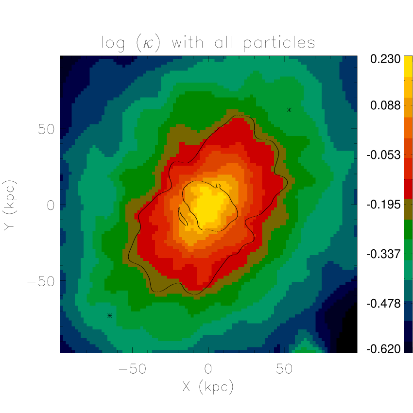
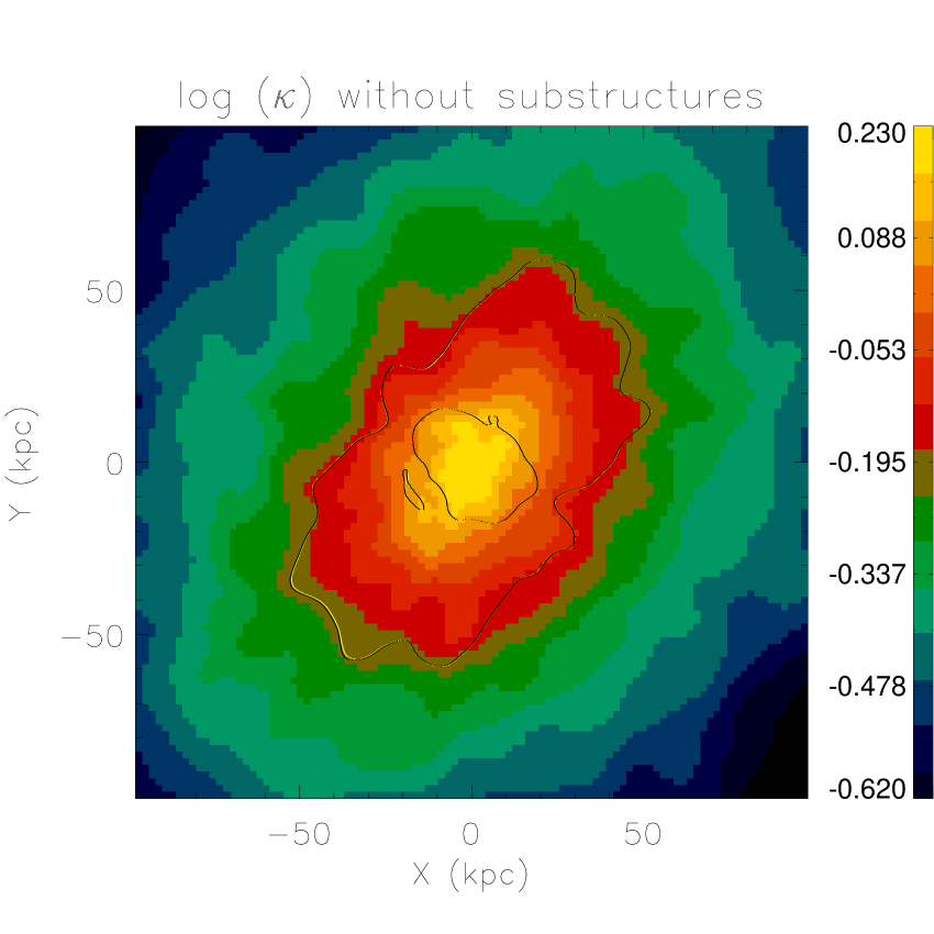
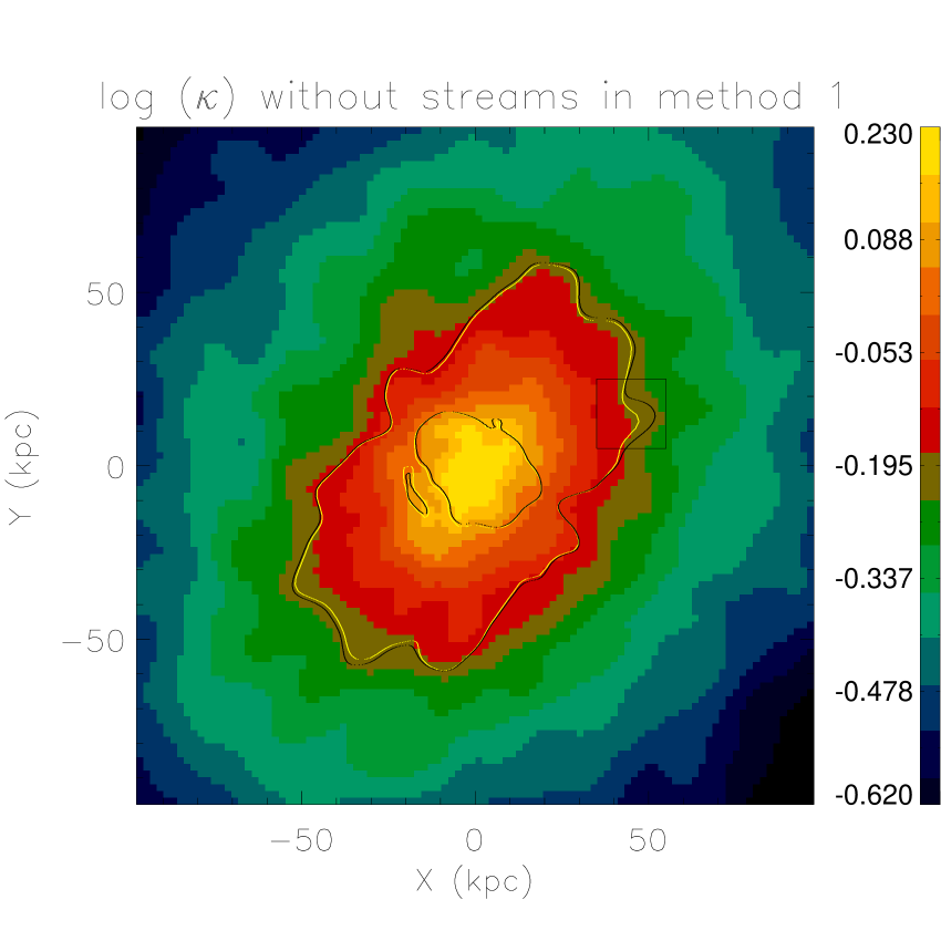
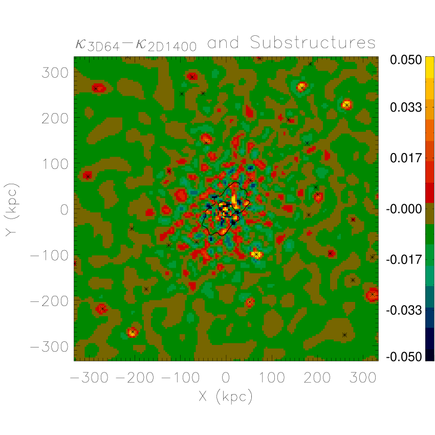
Figure 7: Surface density contours and critical curves (in black and yellow ) for the lensing cluster. a) for all the particles. To facilitate the comparison between the different cases, the critical curves obtained with all particles are repeated as the black curves in the other three panels. b) without bound substructures found by SUBFIND. c) without bound substructures and satellite streams (see Fig. 6) identified in the phase space. d) The difference between the dimensionless surface density obtained using the SI method and the 2D SPH method. The star symbols indicate the position of bound substructures. Notice that the SI method usually gives larger surface densities at the positions of the substructures.

In principle, at least two different algorithms can be used to identify these streams and investigate their influence on higher-order singularities. One is to trace the particles in the phase space (e.g., Helmi et al. 2003; Ascasibar & Binney 2005), while the other is explicitly following the evolution of accreted satellite galaxies. We tried both methods, but the results from these two methods are similar, so we present mainly those from the method where the substructures are identified in the phase space (see below for details). The second (trace-back) method revealed that the cluster consists of two subclusters at redshift unity, which eventually merge to produce the cluster we see at $z=0.3$. The virialization in the cluster formation is however incomplete, as can also be seen from the density contours in Fig. 7.

To identify the satellite streams in the phase space, we first removed the bound substructures we found from the cluster using SUBFIND. All the substructure particles within the lensing box are excluded. The volume density of each particle, $\rho(i)$ is then calculated with the SPH method using 64 neighbors. A characteristic length is defined as ${\rho(i)}^{-1/3}$. Then the Friends-Of-Friends (FOF) algorithm is used to find the structures in the phase space. We find that the density of particles in velocity space is approximately constant as a function of radius, hence a constant linking length in the velocity of $0.2\sigma$ is appropriate, where $\sigma$ is the velocity dispersion for all the particles relative to the cluster center. In the real space, the volume density changes rapidly as a function of position, so we use a variable linking length, $2\times{\rho(i)}^{-1/3}$. Such a linking length allows us to extract a stream that has a volume density a factor of $2^{3}$ smaller than the local volume density, but discards streams with a much lower amplitude. Our method can easily find coherent short-wavelength structures but cannot extract very low-amplitude large-scale features in the phase space. Fig. 6 shows the streams we have found: there are 690 particles in the region with a total mass of $4.28\times 10^{11}h^{-1}M_{\odot}$. This is about 1% of the projection mass in the plotted region ($200\,\rm kpc\times 200\,\rm kpc$) in Fig. 6.

3.3.2 Surface mass density maps, critical curves and caustics

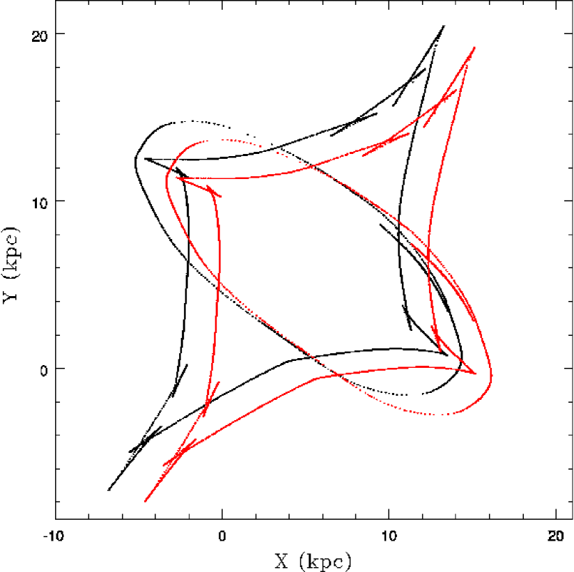
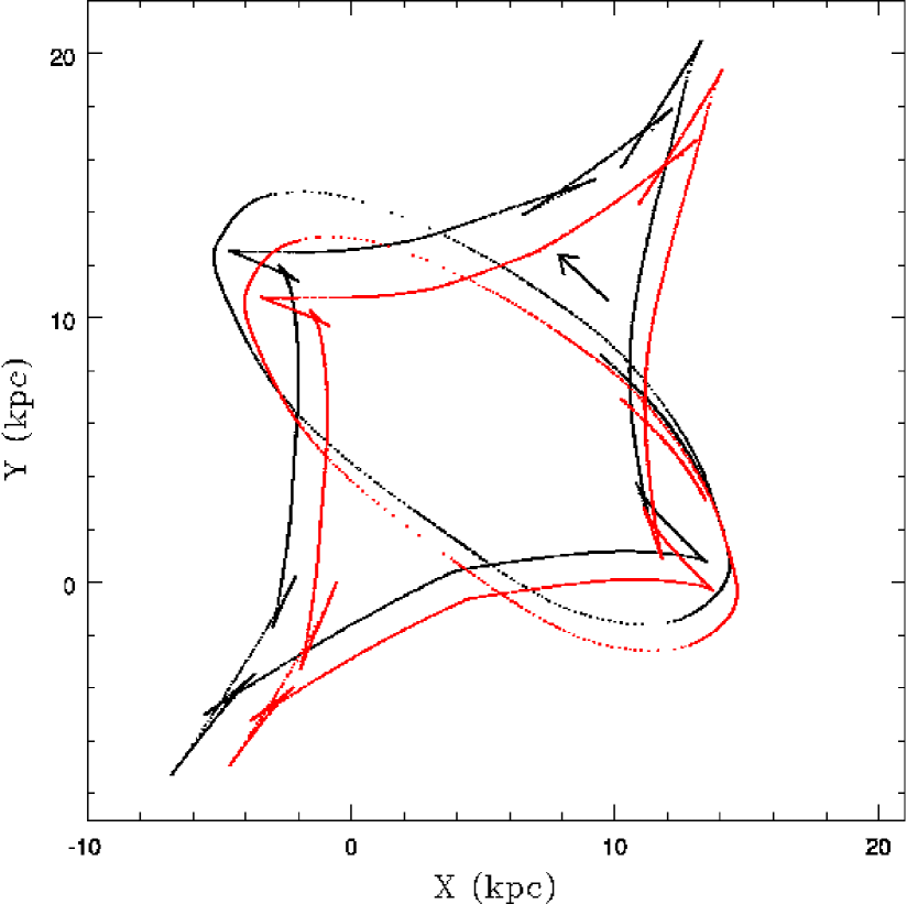
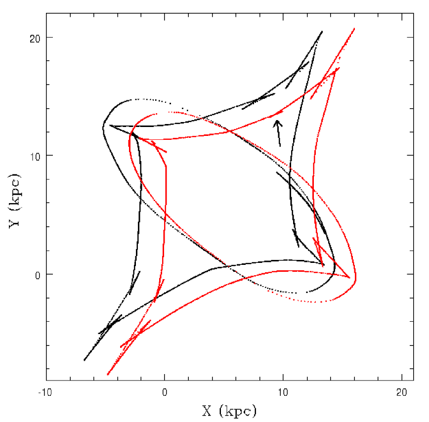
Figure 8: Caustic structures and the probability distribution for $R_{\rm cusp}$. For the top left, right and bottom left panels, the black caustics are obtained using all the particles. The red lines in the two top panels are the corresponding caustics of the top right and bottom left panels in Fig. 7, where we exclude the bound substructures and streams. The top left panel indicates that the substructures in this lens have no effect on high-order singularity regions. The top right panel shows the effect of streams (the most changed region is indicated by the small arrow). A high-order singularity has disappeared because a stream in the position of the small box in the bottom left panel in Fig 6 has been removed. The bottom left panel shows the caustics from the 2D SPH method. Here, the high-order singularity also disappears due to the over-smoothing of the boxed region in the 2D SPH method. The bottom right panel shows the probability distribution of $R_{\rm cusp}$. The 2D SPH smoothing method slightly decreases the probability for high $R_{\rm cusp}$ (see the text).

We now consider the projected surface mass densities with and without substructures and streams using the SI smoothing method in Fig. 7. The number of neighbors in the SI algorithm is set to 64. The top panel in Fig. 7 shows the surface density contours and critical curves when all the particles are included, and the corresponding caustics are shown in the top panel of Fig. 8. The top right panel in Fig. 7 shows the surface density contour when we exclude the bound substructures identified by SUBFIND. The corresponding caustics are shown in Fig. 8. Comparisons show that there is very little difference between the contours of the two sets of surface densities and caustics. The exclusion of streams, however, makes one wiggle in the critical curves less prominent (indicated by a box in the bottom left panel of Fig. 7), and this causes one of the higher-order singularities to disappear. This case can be explained by the stream at (45, 15) kpc identified in Fig. 6. Most wiggles in the critical curves and many perturbations in the surface density plane still remain unchanged. It thus appears that streams (in addition to substructures) can explain one of the high-order singularities for this cluster. However, it looks that the majorities of high-order singularities in this case are caused by other reasons. One possibility is large-scale (low-amplitude) fluctuations in the main halo. Such fluctuations are a natural result of incomplete virialization in the merging process on cluster scales.

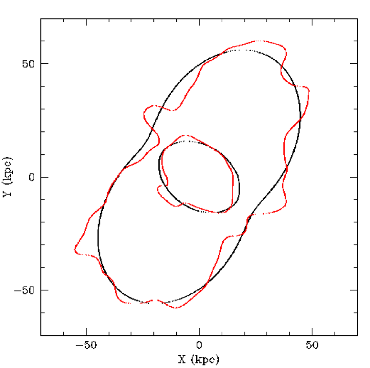
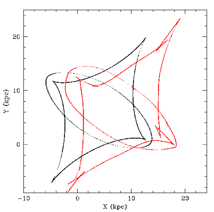
Figure 9: The critical curve (left) and caustics (right) for various approximations for the cluster obtained from cosmological simulations. The black curves in the each panel show the critical curves and cautics for a smooth representation of the cluster and the red curves show that for a Monte Carlo realization of the smooth cluster with the same number of particles as in the cosmological cluster. A high resolution version is available at http://202.127.29.4/mppg/english/data/

However, this may be difficult to prove, as we show below that particle noise can also cause similar levels of high-order singularities. We first fit the density contours as ellipses, and find the radial density profile as a function of the elliptical coordinate, $R_{\rm e}$, where $R_{\rm e}^{2}=x^{2}+y^{2}/q^{2}$ and $q$ is the axial ratio. This creates a smooth representation of our numerical cluster. The critical curve and caustics for this fitted elliptical model are shown in Fig. 9. There are no high-order singularities for this smooth model. We then study the effect of shot noise by populating the fitted smooth elliptical with particles in elliptical annuli. For each annulus, the simulated Monte Carlo cluster has the same number of particles as the numerical one, but the angular positions of particles are randomized. Fig. 9 shows the resulting critical curves and caustics for the Monte Carlo resampled cluster. A number of high-order singularities appear which are clearly due to discrete particle noise (about 4.5% in our case). We return to the issue of noise at the end of this section.

One key objective of a good smoothing algorithm is the ability to maintain the information of substructures. In the bottom panel of Fig. 7, we show the difference in the obtained surface densities for the 2D and 3D SPH smoothing algorithms. To keep roughly the same noise level, 1400 neighours are used in the 2D SPH smoothing based on the condition found by equating eqs. (4) and (3). Following the discussions in §3.1 and §3.2, the noise level in the SI method will in general be lower than that in the 2D SPH smoothing method as the SI method reduces noise due to chance alignments in projection. To show the difference more clearly, pixels with values outside the limits of the color bar are set equal to the upper or lower limit. We can clearly see that most bound structures identified by SUBFIND are located in the positive region, i.e., the SI method picks out these overdense substructures more reliably, i.e., the 2D SPH algorithm may have over-smoothed. We believe this also applies to the central region. There are relatively few bound substructures around the critical curve because most substructures are destroyed by the tidal force. As we mentioned before, we traced the evolution of the cluster out to redshift unity and found that in total 88 progenitors eventually merge to produce the cluster – many of the particles in these clumps are not yet virialized, as can be seen in the satellite streams in Fig. 6. So fluctuations (shown as red) in the inner region are real, highlighting the over-smoothing by the 2D SPH smoothing method.

3.3.3 Cusp relations

Sources close to and inside cusps in general will produce three close images. The properties of such images have been studied theoretically (Blandford & Narayan 1986; Blandford 1990; Schneider & Weiss 1992; Mao 1992 & Zakharov 1995). The magnifications of the three close images follow a simple relation:

$$R_{\rm cusp}=\frac{|{\mu_{\rm A}+\mu_{\rm B}+\mu_{\rm C}}|}{|\mu_{\rm A}|+|\mu_{\rm B}|+|\mu_{\rm C}|}\rightarrow 0,\;{\rm for}\;\mu_{\rm tot}\rightarrow\infty\;,$$ (6)

where A, B and C are three images in the cusp system and $\mu_{\rm tot}$ is the sum of unsigned magnifications of these three images (the denominator in the equation above). Cusp images are more sensitive to the presence of substructures (Mao & Schneider 1998; Keeton, Gaudi, & Petters 2003) than the separation of images or arc numbers. If the lensing potential is smooth, then $R_{\rm cusp}$ must vanish asymptotically as a source gets close to a cusp. We use the cusp relation to check the difference in the lensing properties of the 2D and 3D SPH smoothing algorithms. For a given surface density, the lensing potential is obtained using the FFT method (e.g., Bartelmann et al. 1998; Li et al. 2005). A regular grid is put on the source plane and the Newton-Raphson method is used to find all the images and their corresponding magnifications.

For a source position which produces more than three images, we first determine the polar angles for all the images measured from the cluster center. The opening angle between any two images with the same parity are measured. The two images with the smallest opening angle are selected as the two outer cusp images. The third image can be easily identified as it has the opposite parity and lies inside the two outer cusp images. We restrict cusp systems to the lenses where $\mu_{\rm tot}$ is larger than 30. This is a simple way of selecting systems that have three highly-magnified close images. Fig. 8d shows the probability distribution of $R_{\rm cusp}$ for the 2D and 3D SPH smoothing algorithms. The 2D SPH method decreases the probability for high $R_{\rm cusp}$ because it tends to over-smooth the structures compared with the SI method. However, the most striking result is that the Monte Carlo resampled cluster also produces large deviations, just as seen in the numerical simulated cluster, showing that the noise can mimic the high-order singularities (see Fig. 9). The problem is due to the Poisson noise whose level is still too high, $\sim 4.5\%$. Notice that, to decrease the noise level, we cannot simply increase the number of neighbors in the SI smoothing because this may over-smooth and remove crucial information on substructures and voids.

Of course, we expect the cusp relation to be better satisfied if we increase the number of particles in our volume and approach the limit of a smooth potential. To verify this, we generated a new cluster for which we increase the number of particles by a factor of 16. The mass of each particle is lowered by the same factor so as to keep the total mass of the cluster the same. If we take the $N_{\rm ngb}$ in the 2D SPH smoothing kernel to be $4\times 1400$, then the predicted relation still shows large deviations from the smooth elliptical density distribution (see Fig. 10). However, when $N_{\rm ngb}$ are increased by a factor of 16, the probability distribution of $R_{\rm cusp}$ resembles that of a perfect smooth elliptical distribution. From eq. (4), the noise level drops to about $\approx 1\%$. In this case, the level of noise appears to be low enough to reproduce the theoretically expected cusp magnification relation. According to our comparisons of surface densities with different noise levels, this value is approximately the highest tolerable level for reliably reproducing the cusp relation for this cluster. This means that, in order to suppress the impact of noise or quantify the effect of (sub)structures on the cusp relation, the mass resolution should be increased by a factor of 16. In our case, the particle number, $N_{p}$, should be increased to $\sim 1\times 10^{7}$ or more. Furthermore, $N_{\rm ngb}$ sets a threshold for the smallest (sub)structures that we can resolve reliably. Substructures with $\gtrsim{N_{\rm ngb}}$ particles will be over-smoothed. In other words, for a given lower mass limit of (sub)structures above which we we want to investigate the cusp relation, the particle number needed in simulations can be very approximately estimated using eq. (4) for a desired surface density fluctuation. The best ${N_{\rm ngb}}$ needs to be chosen on the balance of the lowest mass of clumps we want to resolve and the noise level one can tolerate.

3.4 Comparisons with the Delaunay tessellation field estimator

Bradac et al. (2004) presented a detailed study of the lensing properties of a numerically simulated elliptical galaxy (Meza et al. 2003). They used the Delaunay tessellation method in three dimensions to obtain the surface density maps. They also added an external shear and calculated the resulting critical curves, caustics and the cusp relation (cf. eq. 6). In this subsection, we present comparisons between their results and ours for this galaxy.

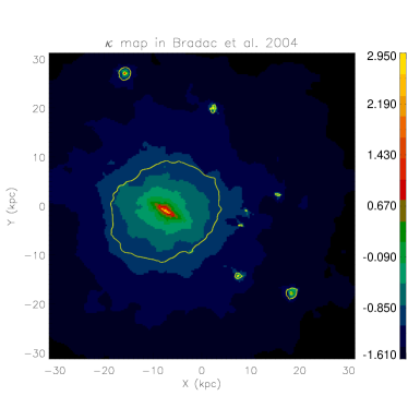
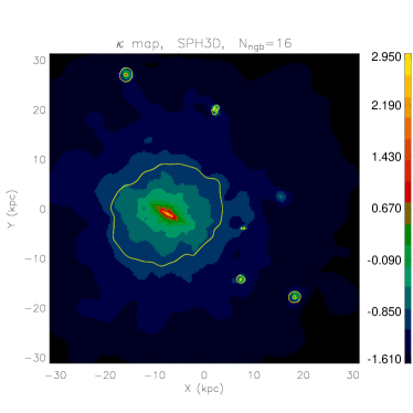
Figure 11: The surface density maps obtained using the Delaunay tessellation field estimator (Bradac et al. 2004, top left panel), and those with the SI method with ${N_{\rm ngb}}=8,16$ and 32. The solid (yellow) line in each panel shows the critical curve.

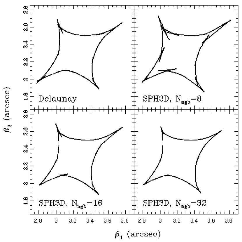
Figure 12: Caustics corresponding to the surface density maps shown in Fig. 11. The top left figure is in good agreement with Fig. 2a in Bradac et al. (2004) obtained using the Delaunay tessellation field estimator. The noise in this map is comparable to that in the SI method for ${N_{\rm ngb}}=16$ in the bottom left panel.

The top left panel of Fig. 11 presents the surface density map and the critical curve for the galaxy projected along the $z$-axis by Bradac et al. (2004). The other three panels show the surface density maps obtained using the SI method with ${N_{\rm ngb}}$=8, 16 and 32. It is clear that the maps are similar, particularly the one with ${N_{\rm ngb}}=16$ seems to match the Bradac et al. surface density map (the top left panel), including the substructures. The ${N_{\rm ngb}}=32$ surface density map may be somewhat over-smoothed, as the clumps appear circular. The corresponding caustics for the four surface density maps are shown in Fig. 12. For the ${N_{\rm ngb}}=16$, the caustics match that obtained through their Delaunay tessellation method quite well. In short our method yields results that are consistent with those obtained with the Delaunay tessellation method.

Bradac et al. (2004) also assessed the reality of high-order singularities and the violation of the cusp relation seen in their simulated galaxy. To do this, they created an ellipsoidal galaxy with a power-law density profile, $\rho(r)\propto r^{-2.9}$. The steep slope is adopted to match that seen in the simulated cluster around the outer critical curve. Their simulated galaxy shows no higher-order singularities and violations of the cusp relation (see their Fig. 8). This is different from our Monte Carlo simulation (see Fig. 10) where violations of the cusp relation (and high-order singularities) seem to persist.

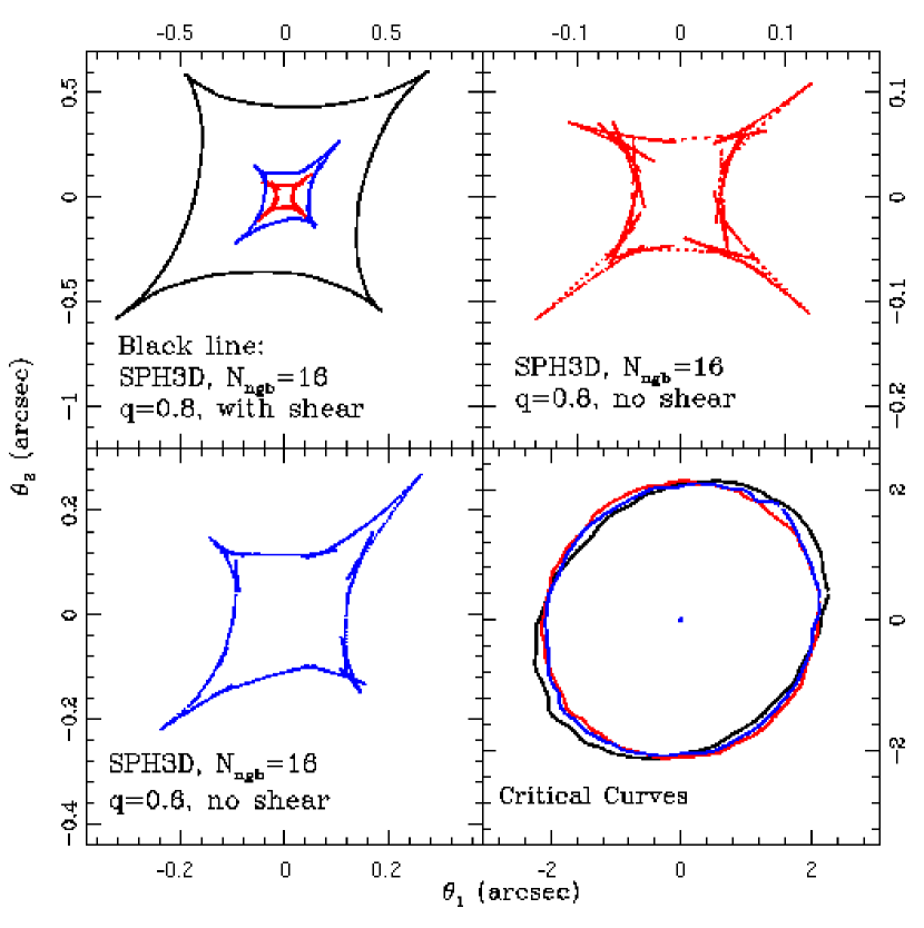
Figure 13: The effect of shear and ellipticity on the caustics and high-order singularities for different realizations of an oblate galaxy projected along one of the major axes. All the galaxies have about 95000 particles within the same box of Bradac et al. (2004) and the density profile is a power-law, $\rho(r)\propto r^{-2.9}$. The major axis has an angle of 45^∘ with respect to the horizontal axis. For the top right and bottom left panels the axis ratios are 0.8 and 0.6 respectively. The black curve in the top left panel has an axis ratio of 0.8 and an external shear (with the same value as in Bradac et al. 2004). Notice how the sizes of caustics and high-order singularities change. In particular, for the black curve (in the top left panel) there are no high-order singularities (see text).

To understand the behavior seen in their simulations, we created several Monte Carlo realizations of a prolate galaxy for different axis ratios and external shear. We use the same number of particles ($\sim 95000$) within the virialized region as they used and the surface density is obtained along the projection of one of the major axes. For the first realization, we use an axis ratio 0.8 and the main axis has an angle of $45^{\circ}$ with respect to the horizontal axis. In this case, the caustics are small and show many high-order singularities (see the top right panel in Fig. 13). If the axis ratio is changed to 0.6 (the bottom left panel), the caustics are a factor of two larger, but the high-order singularities are less important. If we add an external shear (as in Bradac et al. 2004) to the case with an axis ratio of 0.8, then we obtain similar caustics (the black-line in the top left panel of Fig. 13) as the one shown in their Fig. 8a. Notice that the caustics are much larger and there are no more high-order singularities. In all three realizations, the shapes of their critical curves are rather similar (see the bottom panel). This exercise demonstrates that high-order singularities are not only a function of the surface density fluctuations but also the detailed form of the smooth component of the lens potential, including the ellipticity and shear.

A more quantitative understanding can be achieved using the results in Evans & Witt (2001) where they modeled the lensing potential as an isothermal sphere with arbitrary angular dependences (see also Witt, Mao & Keeton 2000). They showed that for galaxies with higher ellipticities (which usually have larger caustic sizes) require a higher level of fluctuations to exhibit higher order singularities (see their Fig. 3 and eq. 32). We believe the difference between our results and those in Bradac et al. can be understood due to the difference in the adopted potential forms. the external shear in their Monte Carlo simulation may act as a large effective ellipticity which enlarges the caustics relative to those seen in our Monte Carlo simulations with ellipticities 0.5 and 0.7. As a result, the importance of high-order singularities may be suppressed with similar fluctuations in the surface densities.

This also explains the difference between Figs. 5 and. 9. The noise levels around the critical curves are quite similar in these two cases (both are around 5%). However, there are no visually striking singularities in the caustics for the isothermal ellipsoid case while for the simulated cluster, higher-order singularities are quite prominent. This arises because for the SIE cluster, the axis ratio is 0.5 while for the numerically simulated cluster, the axis ratio is larger (0.7). The caustic size for the SIE cluster is correspondingly larger. The difference in the axis ratio and caustic sizes means that the same level of fluctuation has different effects on the high-order singularities. We verified that if we adopt a more spherical isothermal cluster (increasing $q_{3}$ close to 1), the caustics becomes smaller. When the axis ratio and caustics are similar to that of the simulated cluster, then at the same noise level, high-order singularities also appear.

4 Summary and Discussions

We have used SPH smoothing algorithms in both 2D and 3D to obtain the surface densities of galaxy clusters. We used Monte Carlo simulations of a uniform density field, an isothermal ellipsoid and an $N$-body numerical cluster to compare these two SPH smoothing algorithms. We find that in general the 3D smoothing algorithm is superior to the smoothing of the 2D projected particle distribution. In particular, our scatter and integrate method, for which we first scatter the particle mass in the nearby grid points in 3D and then integrate to obtain the surface density, appears to reproduce the underlying surface density well. With ${N_{\rm ngb}}=32$ or 64, no prominent artificial higher-order singularities are produced for the isothermal ellipsoid we simulated.

These high-order singularities are particularly important for the anomalous flux ratio problem. As shown by Bradac et al. (2004), these often appear close to the cusps, and produce large cross-sections which violate the cusp relation. For our high-resolution numerical cluster, we have critically examined how these high-order singularities arise. It appears that one of the higher order singularities is related not to bound substructures but to a satellite stream identified in the phase space. For the ten most massive clusters in our $N$-body simulation, we found that there are always one or more compact unbound structures in the inner region of clusters. So the effects of streams may be important for cluster lensing.

Our results show that the importance of high-order singularities will be a sensitive function of the cluster ellipticity and external shears, as also demonstrated by Evans & Witt (2001; see Keeton, Mao & Witt 2000). This implies that the maximum noise level allowed to produce reliable predictions will depend on the detailed form of the lensing potential. Galaxies with small ellipticities are particularly sensitive to the shot noise, and hence will require many more particles to make reliable predictions.

If the high-order singularities are due to true large-scale fluctuations induced, for example, by merging, then their presence is sensitive to the merging state of clusters. As the merger rate likely increases at higher redshift and for the most massive clusters, it will be interesting to examine how these higher-order singularities change as a function of redshift and cluster mass. These higher-order singularities provide regions that can form sextuplet and octuplet images (Keeton, Mao & Witt 2000; Evans & Witt 2001). Evans & Witt (2001) estimated that perhaps $\sim 1\%$ of galaxy-scale lenses may be sextuplet and octuplet imaged systems. This fraction may be higher for clusters because they have much more irregular mass distributions. Upcoming large surveys (e.g., Wittman et al. 2006) will discover a large number of clusters, the chance of seeing these systems may be quite realistic.

It is however less clear whether such high-order singularities should be as prevalent as in galaxies. This is because most lensing galaxies are ellipticals which may have little evolution since redshift of $\sim 1-2$. So the substructures in galaxies may be more effectively destroyed. As even state-of-art simulations cannot reproduce galaxies realistically in a cosmological setting (e.g. Kawata 2001; Westera et al. 2002; Adadi et al. 2003 ), the importance of bound subhaloes and, particularly, streams in numerical simulations remain to be seen.

   

Figure 1: The left panel shows the noise levels of the volume density derived using the SPH kernel in 3D for a uniform volume density field. The different points correspond to different realizations. The solid curve is our empirically derived noise formula, eq. (3). The right panel shows the noise levels for the surface density using the scatter and integrate (SI) algorithm. The solid curve is our empirically derived noise formula, eq. (4).

       

Figure 2: The surface density $\kappa$ and relative standard deviation for the isothermal ellipsoid model as a function of the ellipsoidal radius $R$. The particle mass, the smoothing method and the number of particles used in smoothing are labelled in each panel. The solid curve shows the analytical surface density.

       

       

Figure 4: Same as Fig. 2, but for a particle mass of $0.05\times 10^{10}h^{-1}M_{\odot}$ and a total number of particles, ${N_{\rm p}}=1748982$.

       

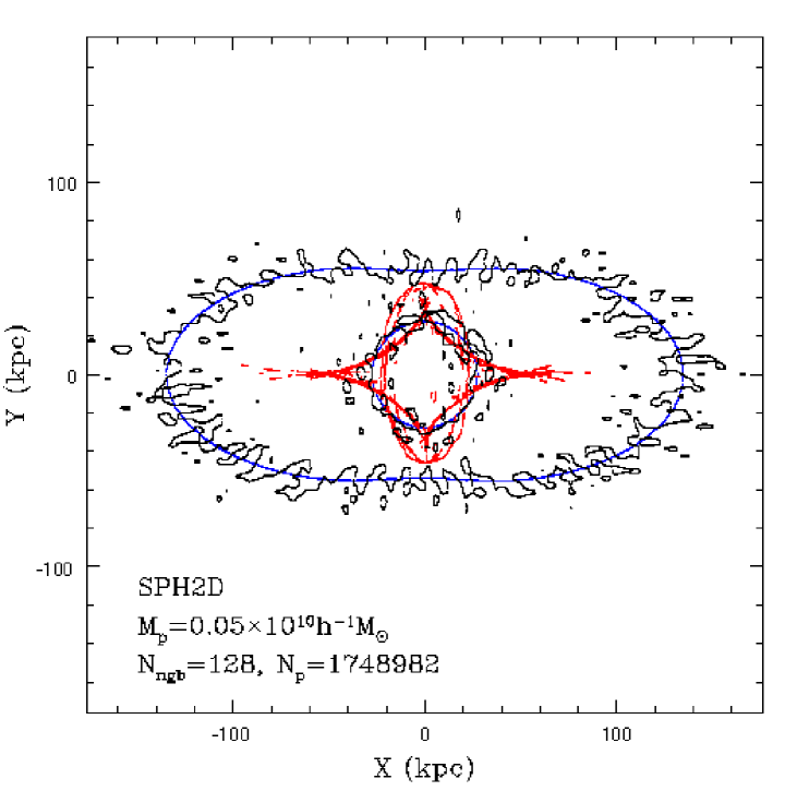
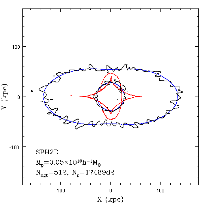
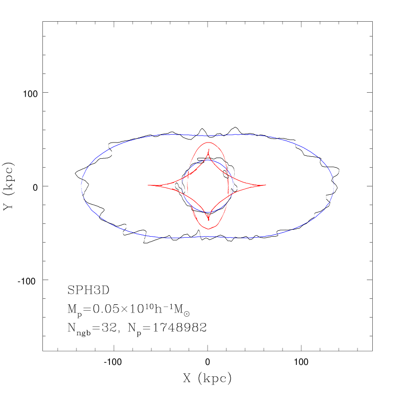
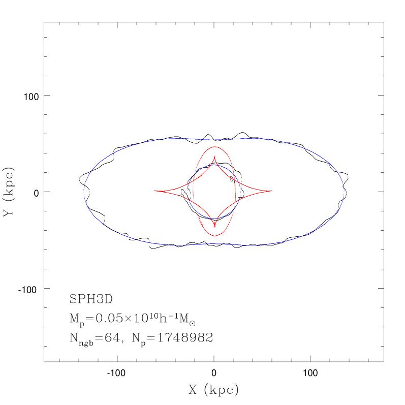
Figure 5: Same as Fig. 3, but for a particle mass of $0.05\times 10^{10}h^{-1}M_{\odot}$ and a total number of particles, ${N_{\rm p}}=1748982$. A high resolution version is available at http://202.127.29.4/mppg/english/data/.

Figure 6: Streams identified in the phase space. There are 690 particles in this region, about 1% of the particles in the plotted region. The small box at (45, 15) kpc indicates the stream that significantly affected one of the higher-order singularities shown in the Fig. 8b and c.

       

       

   

Figure 10: The effect of noise on the cusp relation. The mass resolution is increased by a factor of 16 in the Monte Carlo realization. The number of neighbors in SPH2D is set as 4$\times$1400=5600 and 16$\times$1400=22400. From eq. (4), the noise levels are approximately 2.2% and 1.1% respectively. The distribution for the latter reproduce the theoretical cusp relation for the smooth elliptical (solid line).

References

- (1) Abadi, M. G., Navarro, J. F., Steinmetz, M., & Eke, V. R. 2002, ApJ, 591, 499
- (2) Ascasibar, Y., & Binney, J. 2005, MNRAS, 356, 872
- (3) Bartelmann, M. 2003, gravitational lensing winter school, Aussois, la vieille Europe (astro-0304162)
- (4) Bartelmann, M., Huss, A. Colberg, J. M., Jenkins, A., & Pearce, F. R. 1998, A&A, 330, 1 (B98)
- (5) Bartelmann, M., & Weiss, A. 1994, A&A, 284, 285
- (6) Bartelmann, M., Steimetz, M. & Weiss, A. 1995, A&A, 297, 1
- (7) Bartelmann, M., Meneghetti, M., Perrotta, F., Baccigalupi, C., & Moscardini, L. 2003, A&A, 409, 449
- (8) Blandford, R., & Narayan, R. 1986, ApJ, 310, 568
- (9) Blandford, R. D. 1990, QJRAS, 31, 305
- (10) Bradac, M., Schneider, P., Steinmetz, M., Lombardi, M., King, L. J., & Porcas, R. 2002, A&A, 388, 373
- (11) Bradac, M., Schneider, P., Lombardi, M., Steinmetz, M., Koopmans, L. V. E., & Navarro, J. F. 2004, A&A, 423, 797
- (12) Dalal, N., Holder, G., & Hennawi, J. F. 2004, ApJ, 609, 50
- (13) Evans, N. W., & Witt, H. J. 2001, MNRAS, 327, 1260
- (14) Helmi A., White S. D. M., & Springel V. 2003, MNRAS, 339, 834
- (15) Hernquist, L., & Katz, N. 1989, ApJS, 70, 419
- (16) Hockney, R. W., & Eastwood, J. W. 1981, Computer Simulation Using Particles (McGraw-Hill: New York)
- (17) Jing, Y. P., & Suto Y. 2002, ApJ, 574, 538
- (18) Kawata, D. 2001, ApJ, 558, 598
- (19) Keeton, C. R., Kochanek, C. S. 1998, ApJ, 495, 157
- (20) Keeton, C. R., Mao, S., & Witt, H. J. 2000, ApJ, 537, 697
- (21) Keeton, C. R., Gaudi B. S., & Petters A. O., 2003, ApJ, 598, 138
- (22)
- (23) Kochanek, C. S., 1991, ApJ, 373, 354
- (24) Kochanek, C. S., & Dalal, N. 2005, ApJ, 610, 69
- (25) Kochanek, C.S., Schneider, P., Wambsganss, J., 2004, Gravitational Lensing: Strong, Weak & Micro, Proceedings of the 33rd Saas-Fee Advanced Course, G. Meylan, P. Jetzer & P. North, eds. (Springer-Verlag: Berlin)
- (26) Kormann, R., Schneider, P., & Bartelmann, M. 1994, A&A, 284, 285
- (27) Li, G. L., Mao, S., Jing, Y. P., Kang, X., Bartelmann, M., & Meneghetti, M. 2005, ApJ, 635, 795
- (28) Lombardi, M., Schneider, P., A&A, 392, 1153
- (29) Macciò, A. V., Moore, B., Stadel, J., Diemand J. 2006, MNRAS, 366, 1529
- (30) Macciò, A. V., Miranda, M. 2006, MNRAS, 368, 599
- (31) Mao, S. 1992, ApJ, 389, 63
- (32) Mao, S., & Schneider, P. 1998, MNRAS, 295, 587
- (33) Mao, S., Jing, Y. P., Ostriker, J. P., & Weller, J. 2004, ApJ, 604, 5
- (34) Meneghetti, M., Bolzonella, M., Bartelmann, M., Moscardini, L., & Tormen, G.. 2000, MNRAS, 314, 338
- (35) Meneghetti, M., Bartelmann, M., & Moscardini, L. 2003, MNRAS, 346, 67
- (36) Meneghetti, M., Bartelmann, M., Dolag, K., Moscardini, L., Perrotta, F., Baccigalupi, C., & Tormen, G. 2004, New Astronomy Reviews, 49, 111
- (37) Meza, A., Navarro, J. F., Steinmetz, M., Eke, V. R. 2003, ApJ, 590, 619
- (38) Monaghan, J. 1992, ARAA, 30, 543
- (39) Navarro, J. F., Frenk, C. S., & White, S. D. M. 1997, ApJ, 490, 493
- (40) Niedereiter, H. 1978, Bull. Amer. Math. Soc, 84, 957
- (41) Puchwein, E., Bartelmann, M., Dolag, K., & Meneghetti, M. 2005, A&A, 442, 405
- (42) Schaap, W.E., & van de Weygaert, R. 2000, A&A, 363, L29
- (43) Schneider, P., & Weiss, A. 1992,A&A, 260, 1
- (44) Springel, V., White, S. D. M., Tormen, G., & Kauffmann, G. 2001, MNRAS, 328, 726
- (45) Torri, E., Meneghetti, M., Bartelmann, M., Moscardini, L., Rasia, E., & Tormen, G. 2004, MNRAS, 349, 476
- (46) Wambsganss, J., Bode, P., & Ostriker, J. P.,
- (47) van de Weygaert, R. 1994, A&A, 283, 361 2004, ApJ, 606, L93 (W04)
- (48) Westera, P., Samland, M., Buser, R., & Gerhard, O. E. A&A, 389, 761
- (49) Wittman, D., Dell’Antonio, I. P., Hughes, J. P., Margoniner, V. E., Tyson, J. A., Cohen, J. G., & Norman, D. 2006, ApJ, 643, 128
- (50) Zakharov, A. F. 1995, A&A, 293, 1