Magnetic field confinement by meridional flow and the solar tachocline

We show that the MHD theory that explains the solar tachocline by an effect of the magnetic field can work with the decay modes of a fossil field in the solar interior if the meridional flow of the convection zone penetrates slightly the radiative zone beneath. An equatorward flow of about 10 m/s penetrating to a maximum depth of 1000 km below the convection zone is able to generate almost horizontal field lines in the tachocline region so that the internal field is almost totally confined to the radiative zone. The theory of differential solar rotation indeed provides meridional flows of about 10 m/s and a penetration depth of $\;\buildrel<\over{\scriptstyle\sim}\;$ 1000 km for viscosity values that are characteristic of a stable tachocline.

1 Introduction

While rotation of the solar radiative core is almost uniform, the convection zone rotates differentially (Wilson et al. WBL97 (1997); Kosovichev et al. KSS97 (1997); Shou et al. Sea98 (1998)). The transition from inhomogeneous to rigid rotation occurs in a thin almost spherical layer named ‘tachocline’, whose parameters are well known from helioseismology. The tachocline thickness is estimated to be $\;\buildrel<\over{\scriptstyle\sim}\;$$0.05R_{\odot}$, its midpoint radius is $\left(0.692\pm 0.005\right)R_{\odot}$, and it is slightly prolate in shape (Kosovichev K96 (1996); Antia et al. ABC98 (1998); Charbonneau et al. 1999b ). The tachocline lies totally, or at least mostly, beneath the base of convection zone at $R_{\mathrm{in}}=0.713R_{\odot}$ (Christensen-Dalsgaard et al. CDea91 (1991); Basu & Antia BA97 (1997)), at the very top of the radiative core.

The existence of tachocline is evidence of a link between low and high latitudes that should be present just beneath the convection zone in order to suppress the latitudinal differential rotation. Similarly, uniform rotation in the radius beneath the tachocline indicates that a coupling in radius should be present there. Otherwise, rotational braking of the Sun would leave a rapidly rotating core. Among several theoretical concepts suggested for the solar tachocline, only one that explains it by the effect of a weak internal magnetic field can provide both links simultaneously (Charbonneau & MacGregor CM93 (1993); MacGregor & Charbonneau MC99 (1999)). The uniform rotation of the core was even considered as evidence of an internal field. Another argument by Cowling (C45 (1945)) is that the time of resistive decay for the hypothetical internal field exceeds the solar age.

It has been confirmed by numerical modeling that even a weak ($\sim 10^{-3}$G) poloidal field can produce the tachocline (Rüdiger & Kitchatinov RK97 (1997); MacGregor & Charbonneau MC99 (1999)). However, this is the case only if the field geometry satisfies certain constraint. Ferraro’s (F37 (1937)) law on the constancy of angular velocity along the field lines requires the field to be almost horizontal inside the tachocline region (except, perhaps, for the mid latitudes where angular velocity at the base of convection zone equals that of the bulk of the core).

Why the field should be confined inside the radiative core has remained, however, uncertain. The main idea of the present paper is that the required field geometry may result from the influence of the meridional flow penetrating the radiative core from the convection zone. If the electric conductivity in the radiative core is much higher than in the convection zone, then (and only then) the flow has massive electrodynamical consequences, and the poloidal magnetic field becomes parallel to the meridional flow (cf. Mestel M99 (1999)).

The flow – produced in the convection zone by centrifugal and barocline forcing – only slightly penetrates the radiative core (Gilman & Miesch 2004; Kitchatinov & Rüdiger KR05 (2005)). Its induction can thus be included via the boundary condition. In this paper we formulate the boundary condition for a poloidal field on the top of the radiative core with account for the shallow penetration of meridional flow. With such a modified boundary condition, the modes of the internal poloidal field with the longest decay times are computed. The long-living modes show the required confined structure. The thus defined internal field is then used in tachocline computations to confirm that a slender tachocline can indeed be found.

2 Penetration

The penetration of the meridional flow beneath the solar convection zone was computed by Kitchatinov & Rüdiger (KR05 (2005)). The main results are shown in Fig. 1. The meridional velocity in the penetration region shows reversals with increasing depth, where the flow amplitude reduces largely after each reversal. The penetration depth $D_{\mathrm{pen}}$ in Fig. 1 has been defined as the distance from the base of the convection zone to the location of the first reversal.

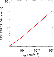
Figure 1: Left: penetration depth as a function of the core viscosity. Right: meridional velocity profile in the penetration region at $45^{\circ}$ latitude for $\nu_{\mathrm{in}}=1.1\cdot 10^{9}$ cm²s^-1. Negative values mean equatorward flow. The vertical dotted line marks the bottom of the convection zone.

The penetration results from viscous drag imposed by the meridional flow at the base of the convection zone on the fluid beneath, and this is opposed by the Coriolis force. The Ekman balance results in the estimation $D_{\mathrm{pen}}\sim\sqrt{\nu_{\mathrm{in}}/\Omega}$ (Gilman & Miesch GM04 (2004), $\nu_{\mathrm{in}}$ is the viscosity in the penetration region, $\Omega$ its basic angular velocity). The plot of Fig. 1 (left) is approximated well by $D_{\mathrm{pen}}\simeq 2.3\sqrt{{\nu_{\mathrm{in}}}/\Omega}$ or, equivalently, by

$$D_{\mathrm{pen}}=1.4\sqrt{\nu_{\mathrm{in}}}\cdot 10^{3}\ \mathrm{cm}$$ (1)

for solar parameters. Thus, the penetration distance is about 100 m for microscopic viscosity and remains smaller than 1 Mm for any reasonable value of eddy viscosity. The penetration depth is small even compared to the tachocline thickness, $D_{\mathrm{pen}}\ll D_{\mathrm{tach}}$.

This shallow penetration may still strongly influence the geometry of an internal poloidal field. The penetration makes a shear flow on the top of the radiative core. The time $\tau_{\mathrm{s}}\simeq D_{\mathrm{p}}/u^{\mathrm{m}}$ of latitudinal field shearing from the radial one is small compared to the time $\tau_{\mathrm{diff}}=D^{2}_{\mathrm{pen}}/\eta_{\mathrm{in}}$ of diffusive escape of the field from the penetration region. The time ratio, $\tau_{\mathrm{diff}}/\tau_{\mathrm{s}}$, gives the magnetic Reynolds number,

$$\mathrm{Rm}=\frac{D_{\mathrm{pen}}u^{\mathrm{m}}}{\eta_{\mathrm{in}}}\simeq\frac{\mathrm{Pm}}{\sqrt{\nu_{\mathrm{in}}}}10^{6},$$ (2)

where Pm is the magnetic Prandtl number. The value $u^{\mathrm{m}}\simeq 10$ m s^-1 is used for the meridional velocity. With microscopic diffusivities, the number is large, $\mathrm{Rm}\sim 10^{3}$, and it remains higher than this value with eddy diffusivities up to $10^{6}$ cm² s^-1. It sinks to unity for eddy diffusivities of about $10^{12}$ cm² s^-1, so that only in this case does the influence of a penetrating meridional flow on the magnetic field geometry turn weak.

The shearing of the poloidal field is probably the only process where this penetration is important. The advection time, $\tau_{\mathrm{adv}}=R_{\mathrm{in}}/u^{\mathrm{m}}$, is much longer than the diffusion time $\tau_{\mathrm{diff}}$,

$$\frac{\tau_{\mathrm{diff}}}{\tau_{\mathrm{adv}}}=\frac{D_{\mathrm{pen}}}{R_{\mathrm{in}}}\ \ \mathrm{Rm}\simeq 0.03\cdot\mathrm{Pm}\ll 1,$$ (3)

independent of whether microscopic or eddy diffusion applies. Rüdiger et al. (RKA (2005)) argued that the tachocline region should be stable in the hydrodynamic regime so that microscopic diffusivities have to be used. In any case the diffusion time is so short that the penetration layer is not dynamo-relevant (Rüdiger et al. 2005).

3 The model

Axial symmetry for both magnetic and velocity fields is assumed. In spherical coordinates $\left(r,\theta,\phi\right)$, the fields can be written as

$${\@vec{u}}=\left(\frac{1}{\rho r^{2}\sin\theta}\frac{\partial\psi}{\partial\theta},\frac{-1}{\rho r\sin\theta}\frac{\partial\psi}{\partial r},r\sin\theta\ \Omega\right),$$ (4)

$${\@vec{B}}=\left(\frac{1}{r^{2}\sin\theta}\frac{\partial A}{\partial\theta},\frac{-1}{r\sin\theta}\frac{\partial A}{\partial r},\ B\ \right),$$ (5)

in terms of the stream function ($\psi$) of the meridional flow and the potential ($A$) of the poloidal field. Here $\Omega$ is the angular velocity and $B$ the toroidal field.

The poloidal field equation,

$$\frac{\partial A}{\partial t}=-\frac{u_{\theta}}{r}\frac{\partial A}{\partial\theta}-u_{r}\frac{\partial A}{\partial r}+\eta\frac{\partial^{2}A}{\partial r^{2}}+\frac{\eta}{r^{2}}\sin\theta\frac{\partial}{\partial\theta}\left(\frac{1}{\sin\theta}\frac{\partial A}{\partial\theta}\right),$$ (6)

decouples from other equations of the problem. As the eddy diffusivity in the convection zone is large compared to $\eta_{\mathrm{in}}$, the vacuum boundary condition can be applied to the top of the core. The (nonlocal) condition,

$$\frac{\partial A}{\partial r}=\left(\frac{\partial A}{\partial r}\right)_{\mathrm{vac}}\ \ \ {\rm at}\ \ \ r=R_{\mathrm{in}},$$ (7)

is usually expressed in terms of the Legendre polynomial expansion

$$A\left(r,\theta\right) = \sin\theta\sum\limits_{n=1}^{\infty}A_{n}\left(r\right)P_{n}^{1}\left(\cos\theta\right),$$

$$\left(\frac{\partial A}{\partial r}\right)_{\mathrm{vac}} = -\frac{\sin\theta}{r}\sum\limits_{n=1}^{\infty}nA_{n}\left(r\right)P_{n}^{1}\left(\cos\theta\right).$$ (8)

The internal magnetic field can be defined by solving Eq. (6) with the boundary condition (7). The meridional flow is, however, only present in the very thin penetration layer (Fig. 1). Instead of resolving this layer explicitly, we integrate Eq. (6) across the layer to obtain a new boundary condition for the poloidal field for the base of the penetration layer that is still above the tachocline. The effect of penetration is then included in the reformulated boundary condition.

3.1 Poloidal field boundary condition

Inside the penetration layer, the advection time ($\sim 10$ yr) is short compared to the latitudinal diffusion time, $R^{2}_{\mathrm{in}}/\eta_{\mathrm{in}}\sim 10^{9}$ yr. The left part of Eq. (6) and its last term can thus be neglected compared to the first term on the right.

Also, the radial velocity in the penetration layer is small compared to the latitudinal velocity, $u_{r}\sim u_{\theta}D_{\mathrm{pen}}/R_{\mathrm{in}}$ (Gilman & Miesch GM04 (2004)). By neglecting these small terms the equation for the penetration region reads

$$\frac{\partial^{2}A}{\partial r^{2}}+\frac{1}{\eta\rho R_{\mathrm{in}}^{2}\sin\theta}\frac{\partial\psi}{\partial r}\frac{\partial A}{\partial\theta}=0,$$ (9)

where $u_{\theta}$ is expressed in terms of the stream function of Eq. (4). The stream function varies from zero at the base of the layer to a finite value at its top. Divergence-free of magnetic field requires a variation in the radial field, $B_{r}=(\partial A/\partial\theta)/(R^{2}_{\mathrm{in}}\sin\theta)$, across the layer be small. Integration of Eq. (9) across the layer then yields

$$\frac{\partial A}{\partial r}-\frac{\psi(R_{\rm in},\theta)}{\eta_{\mathrm{in}}\rho R_{\mathrm{in}}^{2}\sin\theta}\frac{\partial A}{\partial\theta}=\left(\frac{\partial A}{\partial r}\right)_{\mathrm{vac}},$$ (10)

where $\psi(R_{\rm in},\theta)$ is the stream function profile at the base of the convection zone. The stream function scales as

$$\psi(R_{\rm in},\theta)=u^{\mathrm{m}}\rho R_{\mathrm{in}}D_{\mathrm{pen}}\hat{\psi}(\theta),$$ (11)

where $\hat{\psi}$ is a dimensionless function of order one. Substitution of (11) into (10) leads to the boundary condition sought for the poloidal field,

$$R_{\mathrm{in}}\frac{\partial A}{\partial r}-\mathrm{Rm}\frac{\hat{\psi}\left(\theta\right)}{\sin\theta}\frac{\partial A}{\partial\theta}=R_{\mathrm{in}}\left(\frac{\partial A}{\partial r}\right)_{\mathrm{vac}},$$ (12)

which accounts for the shallow penetration of the meridional flow from the convection zone into the radiative interior.

3.2 Model equations

Any meridional flow in the bulk of radiative core is neglected. The characteristic time of the Eddington-Sweet circulation exceeds the solar age (Tassoul T00 (2000)). The slow circulation may affect the internal field structure but the effect remains small (Garaud G02 (2002)).

The global modes of the internal poloidal field of the core can be computed by solving the eigenvalue equation,

$$-\frac{A}{\tau}=\eta\frac{\partial^{2}A}{\partial r^{2}}+\frac{\eta}{r^{2}}\sin\theta\frac{\partial}{\partial\theta}\left(\frac{1}{\sin\theta}\frac{\partial A}{\partial\theta}\right),$$ (13)

with the boundary condition (12). The other condition requires the solution to be regular at the center. We are interested in the solutions with the longest decay times, $\tau$.

The radial profiles of the microscopic diffusivities and density were defined after the solar structure model by Stix & Skaley (SS90 (1990), see Rüdiger & Kitchatinov RK97 (1997)). All the computations concern the simplest example of a stream function,

$$\hat{\psi}\left(\theta\right)=-\sin\theta\bar{P}^{1}_{2}\left(\cos\theta\right),$$ (14)

where $\bar{P}^{1}_{2}$ is the normalized Legendre polynomial. Equation (14) describes a flow at the base of the convection zone from the poles to the equator, which appeared in all our previous models for the solar differential rotation.

To describe the poloidal field geometry, the ‘escape parameter’,

$$\delta\phi=\frac{\mathrm{max}|A\left(r,\theta\right)|_{r=R_{\mathrm{in}}}}{\mathrm{max}|A\left(r,\theta\right)|_{r\leq R_{\mathrm{in}}}},$$ (15)

is used. The value of $2\pi A\left(r,\theta\right)$ equals the magnetic flux pervading a surface bounded by the longitudinal circle of constant $r$ and $\theta$. The $\delta\phi$-parameter (15) estimates the ratio of the magnetic flux through the surface of the core to the characteristic value of the flux inside the core. The poloidal fields with small $\delta\phi$ are expected to produce the tachocline. Linear equation (13) leaves the amplitude of the field indefinite. The amplitude, $B_{0}$, defined as the maximum strength of poloidal field within the core, remains a free parameter of the model.

With a given poloidal field, the tachocline can be computed by solving the equation system for the toroidal field and angular velocity,

$$\frac{\eta}{r}\frac{\partial}{\partial\theta}\left(\frac{1}{\sin\theta}\frac{\partial\left(B\sin\theta\right)}{\partial\theta}\right)+\frac{\partial}{\partial r}\left(\eta\frac{\partial\left(Br\right)}{\partial r}\right)=\frac{\partial\Omega}{\partial\theta}\frac{\partial A}{\partial r}-\frac{\partial\Omega}{\partial r}\frac{\partial A}{\partial\theta},$$

$$\frac{\rho\nu}{\sin^{3}\theta}\frac{\partial}{\partial\theta}\left(\sin^{3}\theta\frac{\partial\Omega}{\partial\theta}\right)+\frac{1}{r^{2}}\frac{\partial}{\partial r}\left(r^{4}\rho\nu\frac{\partial\Omega}{\partial r}\right)=$$

$$=\frac{1}{4\pi r^{2}\sin^{3}\theta}\left(r\frac{\partial A}{\partial r}\frac{\partial\left(B\sin\theta\right)}{\partial\theta}-\sin\theta\frac{\partial A}{\partial\theta}\frac{\partial\left(Br\right)}{\partial r}\right).$$ (16)

The neglect of the meridional flow in these equations is justified by the small value of parameter (3). The upper boundary conditions require a zero toroidal field and the angular velocity profile

$$\Omega=2.9\left(1-0.15\cos^{2}\theta\right)\ \ \ \mu\mathrm{rad}\ \mathrm{s}^{-1}$$ (17)

favored by the helioseismology for the bottom of the convection zone (Charbonneau et al. 1999a ).

We applied a Legendre polynomial expansion in $\theta$ to Eqs. (13) and (16) and solved the resulting system of ordinary differential equations numerically with the relaxation method.

4 Results and discussion

Figures 2 and 3 illustrate the effect of the penetrating meridional flow on the structure of the longest-living dipolar mode of an internal poloidal field. The internal field of Fig. 2 computed without penetration ($\rm Rm=0$) has an ‘open’ structure. The field computed with $\rm Rm=1000$ has the ‘confined’ geometry required for tachocline formation. Figure 3 shows the dependence of the escape parameter (15) on Rm. For $\rm Rm=1000$, less than 1% of magnetic flux of the dipolar eigenmode escapes the core.

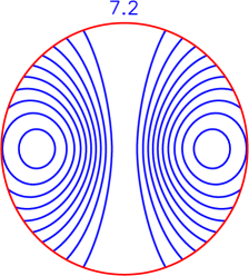
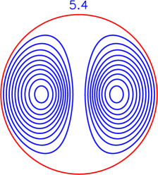
Figure 2: Field lines of the longest-living modes of poloidal field without ($\rm Rm=0$, left) and with penetration ($\rm Rm=1000$, right). The outer circle is the base of the convection zone. Lifetimes of the fields in Gyr are given at the top.

The decay time of the longest-living mode of internal field exceeds the solar age. The lifetime decreases with Rm but approaches a constant value of about 5.4 Gyr for large Rm. The characteristic time of the tachocline formation, $\sim R_{\mathrm{in}}/V_{\mathrm{A}}\sim 10^{4}/B_{0}$ yr ($V_{\mathrm{A}}$ is Alfvén velocity, $B_{0}$ is the field amplitude in Gauss) is much shorter. This justifies using steady poloidal fields in the tachocline computations.

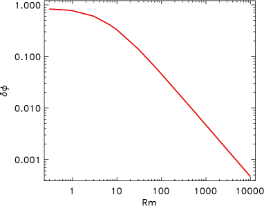
Figure 3: Geometry parameter (15) for the longest-living dipolar mode of the internal field as a function of the magnetic Reynolds number (2). The field becomes increasingly confined to the core as Rm grows.

Figure 4 shows the angular velocity distributions inside the core computed for poloidal fields of Fig. 2. As expected, only the confined field produces a tachocline. The dipolar eigenmode for the solar value of ${\rm Rm}=1000$ is ‘sufficiently confined’ to do so. Already ${\rm Rm}=100$ suffices for the tachocline formation. We conclude that the shallow penetration of the meridional flow into the radiative core influences the internal field geometry so strongly that it becomes appropriate for tachocline formation. We suggest that a layer of less than 1000 km beneath the convection zone, where a meridional flow on the order of 1–10 m/s enters the radiative core, is responsible for the existence of the impressive phenomenon of the solar tachocline (which implies that the bulk of the solar core rotates rigidly).

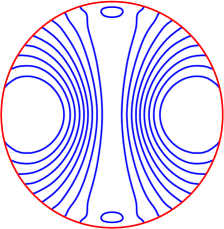
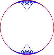
Figure 4: Angular velocity isocontours inside the radiative zone computed with the internal fields of Fig. 2. Left: $\rm Rm=0$, right: $\rm Rm=1000$. $B_{0}=3$ mG.

Analytical estimations suggest that the (fractional) tachocline thickness is controlled solely by the Hartmann number, $\mathrm{Ha}=V_{\mathrm{A}}R_{\mathrm{in}}/\sqrt{\eta_{\mathrm{in}}\nu_{\mathrm{in}}}$,

$$D_{\mathrm{tach}}/R_{\odot}\sim\mathrm{Ha}^{-1/2}$$ (18)

(Rüdiger & Kitchatinov RK97 (1997)). After Eq. (18), even a weak internal field can produce the tachocline. The angular velocity distributions of Fig. 4 were computed for a field amplitude of 3 mG. Figure 5 shows the fractional depth inside the core at which the angular velocity difference between equator and poles drops e-times. When the field is not too weak, the tachocline thickness varies as $D_{\mathrm{tach}}\sim B_{0}^{-1/2}$ in agreement with (18). The thickness falls below 4% of the solar radius at $B_{0}=10^{-2}$ G. The toroidal field in the present model is almost independent of $B_{0}$, and its amplitude is not large, $B_{\mathrm{tor}}\sim 100$ G. The maximum toroidal field within the core is about 140 G for ${\rm Rm}=1000$.

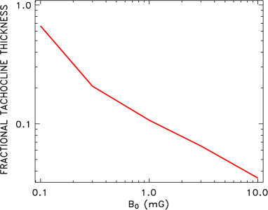
Figure 5: Dependence of the thickness of the tachocline on the amplitude, $B_{0}$, of the internal poloidal field. The thickness is defined as the depth of an exponential reduction in the pole-equator difference of the angular velocity.

The dipolar mode of Fig. 2 has the longest lifetime. The following modes in order of decreasing lifetime are shown in Fig. 6. The lifetimes are shorter than the solar age but not by much. The modes may be mixed in the internal field. Tachocline computations were made for all modes of Fig. 6, and all the field configurations lead to a slender tachocline.

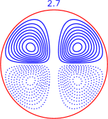
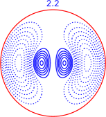
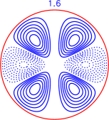
Figure 6: Eigenmodes of the internal field following the dipolar mode of Fig. 2 in order of decreasing lifetime. The lifetimes in Gyr are given at the top. $\rm Rm=1000$. The geometry parameter (15) varies as 0.0051, 0.0073, 0.0026 from left to right.

It is important for this model that the magnetic Reynolds number (2) be large, which is true for microscopic diffusivities or for eddy diffusivities that are not too large, up to about $10^{8}$ cm² s^-1. The tachocline should thus be stable or only mildly turbulent in order to allow sufficiently large Rm.

Another necessary condition is the presence of a meridional flow of about 10 m s^-1 at the bottom of the convection zone. This flow should, of course, be present in the deep convection zone in order to penetrate below its base. Such a flow is also a key ingredient in the advection-dominated solar dynamo models (Wang et al. WSN91 (1991); Choudhuri et al. CSD95 (1995); Dikpati & Gilman DG01 (2001); Bonanno et al. Bea02 (2002)). The flow was predicted by theoretical modeling (Kitchatinov & Rüdiger KR99 (1999); Miesh et al. Mea00 (2000)), but not yet confirmed by any other means. Probing for the deep meridional flow may be a challenge for helioseismology.

The polar cusp in the tachocline of Fig. 4 (right) is a consequence of the assumed axial symmetry. This symmetry is, of course, an idealization. We expect, though so far only on qualitative grounds, that i) the meridional flow penetration can also confine a nonaxisymmetric field to the core and ii) the confined nonaxisymmetric field can also produce the characteristic tachocline structure. An important question is still open as to whether the axisymmetric solutions are stable against nonaxisymmetric disturbances. Purely toroidal fields (Tayler T73 (1973)), as well as the poloidal fields (Wright W73 (1973); Markey & Tayler MT73 (1973)), are known to be unstable near their neutral lines if the fields are sufficiently strong, so that the characteristic time of an Alfven wave passage across the star is shorter than the rotation period. The weak fields of the present model belong to the opposite limit.

- (1) Antia, H. M., Basu, S., & Chitre, S. M. 1998, MNRAS, 298, 543
- (2) Basu, S., & Antia, H. M. 1997, MNRAS, 287, 189
- (3) Bonanno, A., Elstner, D., Rüdiger, G., & Belvedere, G. 2002, A&A, 390, 673
- (4) Charbonneau, P., & MacGregor, K. B. 1993, ApJ, 417, 762
- (5) Charbonneau, P., Dikpati, M., & Gilman, P. A. 1999a, ApJ, 526, 523
- (6) Charbonneau, P., Christensen-Dalsgaard, J., Henning, R. et al. 1999b, ApJ, 527, 445
- (7) Choudhuri, A. R., Schüssler, M., & Dikpati, M. 1995, A&A, 303, L29
- (8) Christensen-Dalsgaard, J., Gough, D. O., & Thompson, M. J. 1991, ApJ, 378, 413
- (9) Cowling, T. G. 1945, MNRAS, 105, 166
- (10) Dikpati, M., & Gilman, P. A. 2001, ApJ, 559, 428
- (11) Ferraro, V. C. A. 1937, MNRAS, 97, 458
- (12) Garaud, P. 2002, MNRAS, 329, 1
- (13) Gilman, P. A., & Miesch, M. S. 2004, ApJ, 611, 568
- (14) Kitchatinov, L. L., & Rüdiger, G. 1999, A&A, 344, 911
- (15) Kitchatinov, L. L., & Rüdiger, G. 2005, Astron. Nachr., 326, 379
- (16) Kosovichev, A. G 1996, ApJ, 469, L61
- (17) Kosovichev, A. G., Schou, J., & Sherrer, P. H. 1997, Sol. Phys., 170, 43
- (18) MacGregor, K. B., & Charbonneau, P. 1999, ApJ, 519, 911
- (19) Markey, P., & Tayler, R. J. 1973, MNRAS, 163, 77
- (20) Mestel, L. 1999, Stellar Magnetism (Clarendon Press)
- (21) Miesch, M. S., Elliott, J. R., Toomre, J., et al. 2000, ApJ, 532, 593
- (22) Rüdiger, G., & Kitchatinov, L. L. 1997, Astron. Nachr., 318, 273
- (23) Rüdiger, G., Kitchatinov, L. L., & Arlt, R. 2005, A&A, 444, 53
- (24) Schou, J., Antia, H. M., Basu, S., et al. 1998, ApJ, 505, 390
- (25) Stix, M., & Skaley, D. 1990, A&A, 232, 234
- (26) Tassoul, J.-L. 2000, Stellar rotation (Cambridge University Press)
- (27) Tayler, R. J. 1973, MNRAS, 161, 365
- (28) Wang, Y.-M., Sheeley, N. R. Jr., & Nash, A. G. 1991, ApJ, 383, 431
- (29) Wilson, P. R., Burtonclay, D., & Li, Y. 1997, ApJ, 489, 395
- (30) Wright G. A. E. 1973, MNRAS, 162, 339