Broad-band photometric colors and effective temperature calibrations for late-type giants. II. Z$<$0.02

We investigate the effects of metallicity on the broad-band photometric colors of late-type giants, and make a comparison of synthetic colors with observed photometric properties of late-type giants over a wide range of effective temperatures ($T_{\rm eff}=3500-4800$ K) and gravities ($\log g=0.0-2.5$), at $\left[\mathrm{M}/\mathrm{H}\right]=-1.0$ and $-2.0$. The influence of metallicity on the synthetic photometric colors is small at effective temperatures above $\sim 3800$ K, but the effects grow larger at lower $T_{\rm eff}$, due to the changing efficiency of molecule formation which reduces molecular opacities at lower $\left[\mathrm{M}/\mathrm{H}\right]$. To make a detailed comparison of the synthetic and observed photometric colors of late type giants in the $T_{\rm eff}$–color and color–color planes (which is done at two metallicities, $\left[\mathrm{M}/\mathrm{H}\right]=-1.0$ and $-2.0$), we derive a set of new $T_{\rm eff}$–$\log g$–color relations based on synthetic photometric colors, at $\left[\mathrm{M}/\mathrm{H}\right]=-0.5$, $-1.0$, $-1.5$, and $-2.0$. These relations are based on the $T_{\rm eff}$–$\log g$ scales that we derive employing literature data for 152 late-type giants in 10 Galactic globular clusters (with metallicities of the individual stars between $\left[\mathrm{M}/\mathrm{H}\right]=-0.7$ and $-2.5$), and synthetic colors produced with the PHOENIX, MARCS and ATLAS stellar atmosphere codes. Combined with the $T_{\rm eff}$–$\log g$–color relations at $\left[\mathrm{M}/\mathrm{H}\right]=0.0$ (Kučinskas et al. 2005), the set of new relations covers metallicities $\left[\mathrm{M}/\mathrm{H}\right]=0.0\dots-2.0$ ($\Delta\left[\mathrm{M}/\mathrm{H}\right]=0.5$), effective temperatures $T_{\rm eff}=3500\dots 4800$ K ($\Delta T_{\rm eff}=100$ K), and gravities $\log g=-0.5\dots 3.0$. The new $T_{\rm eff}$–$\log g$–color relations are in good agreement with published $T_{\rm eff}$–color relations based on observed properties of late-type giants, both at $\left[\mathrm{M}/\mathrm{H}\right]=-1.0$ and $-2.0$. The differences in all $T_{\rm eff}$–color planes are typically well within $\sim 100$ K. We find, however, that effective temperatures predicted by the scales based on synthetic colors tend to be slightly higher than those resulting from the $T_{\rm eff}$–color relations based on observations, with the offsets up to $\sim 100$ K. This is clearly seen both at $\left[\mathrm{M}/\mathrm{H}\right]=-1.0$ and $-2.0$, especially in the $T_{\rm eff}$–$(B-V)$ and $T_{\rm eff}$–$(V-K)$ planes. The consistency between $T_{\rm eff}$–$\log g$–color scales based on synthetic colors calculated with different stellar atmosphere codes is very good, with typical differences being well within $\Delta T_{\rm eff}\sim 70$ K at $\left[\mathrm{M}/\mathrm{H}\right]=-1.0$ and $\Delta T_{\rm eff}\sim 40$ K at $\left[\mathrm{M}/\mathrm{H}\right]=-2.0$.

1 Introduction

Stars on the red giant branch and asymptotic giant branch (RGB and AGB, respectively) are important constituents of intermediate age and old stellar populations. In this age range they contribute significantly to the total radiative energy output of a given population, especially at near-infrared wavelengths (e.g., Mouhcine & Lançon 2002). A realistic representation of the atmospheres and observed spectral properties of late-type giants with current stellar atmosphere models is, therefore, of crucial importance, both for understanding evolution of single stars and stellar systems. This is especially vital for the studies of distant stellar populations which have to rely on the most luminous stars, and frequently on RGB and AGB stars alone.

While theoretical modeling of late-type giant atmospheres has undergone significant development during the last decade, with major improvements in the modeling procedure, current stellar atmosphere models still use a number of simplifications in the model physics and other assumptions (see, e.g., Gustafsson 2003). Indeed, the atmospheres of late-type giants are complex, thus detailed modeling of certain physical phenomena (convection, pulsations, shock waves, grain formation, mass loss) should ideally be done using 3-D radiation hydrodynamics. Obviously, while the classical 1-D model atmospheres may still be very valuable in providing the time-averaged properties of late-type giants (for instance, their broad-band photometric colors), it is important to know how well these theoretically predicted quantities reproduce the observations of real stars.

In the first paper of this series (Kučinskas et al. 2005, Paper I) we made a detailed comparison of synthetic photometric colors produced using current stellar model atmosphere codes (PHOENIX, MARCS, and ATLAS) with observations of late-type giants in the Solar neighborhood, at Solar metallicity. Generally, we found that observed and theoretical colors agree at the level of $\pm 100$ K, over a wide range of effective temperatures ($T_{\rm eff}=3000\dots 4800$ K) and gravities ($\log g=0.0\dots+3.0$; see Paper I for a detailed discussion). Here we extend this analysis to sub-Solar metallicities, assuming Solar-scaled abundances of individual chemical species at $\left[\mathrm{M}/\mathrm{H}\right]<0$.

There are 3 parts of this paper. First, we investigate the influence of metallicity, $\left[\mathrm{M}/\mathrm{H}\right]$, on the synthetic broad-band photometric colors calculated with the PHOENIX stellar model atmosphere code. Second, we derive a set of new $T_{\rm eff}$–$\log g$ relations at different metallicities, based on the published spectroscopic effective temperatures and gravities of 152 giants in Galactic globular clusters. We further employ these relations to derive three new $T_{\rm eff}$–$\log g$–color scales based on the synthetic colors of PHOENIX, MARCS and ATLAS, for $\left[\mathrm{M}/\mathrm{H}\right]=-0.5$, $-1.0$, $-1.5$, and $-2.0$. Finally, we provide a detailed comparison of the new $T_{\rm eff}$–$\log g$–color scales based on the synthetic photometric colors with a number of $T_{\rm eff}$–color relations available from the literature. This comparison is done for two metallicities, $\left[\mathrm{M}/\mathrm{H}\right]=-1.0$ and $-2.0$.

The paper is structured as follows. In Sect. 2 we briefly describe synthetic spectra calculated with the PHOENIX, MARCS and ATLAS model atmospheres, and outline the procedure used to calculate synthetic photometric colors. The effects of metallicity on the photometric colors are discussed in Sect. 3. The new $T_{\rm eff}$–$\log g$ scales for different metallicities are derived in Sect. 4. Here we also discuss a sample of Galactic globular cluster giants which is employed in the derivation of the $T_{\rm eff}$–$\log g$ relations. Finally, the new $T_{\rm eff}$–$\log g$–color relations based on the synthetic colors of PHOENIX, MARCS, and ATLAS are derived in Sect. 5. A comparison of the new $T_{\rm eff}$–$\log g$–color scales with $T_{\rm eff}$–color relations available in the literature is also provided.

2 Stellar atmosphere models, spectra and synthetic colors of late-type giants

The comparison of synthetic photometric colors with observations of late-type giants made in Sect. 5 utilizes colors calculated with the PHOENIX, MARCS, and ATLAS model atmospheres. A detailed description of the model atmosphere codes can be found in relevant papers (PHOENIX: Hauschildt et al. (2003) and references therein; ATLAS: Castelli & Kurucz (2003); MARCS: Plez (2003) and Gustafsson et al. (2003)). In the following subsections we briefly summarize only the most crucial issues related to the calculation of synthetic spectra and broad-band photometric colors.

2.1 PHOENIX spectra and broad-band colors

PHOENIX photometric colors used in this work were calculated in Paper I employing a new grid of PHOENIX spectra. This grid is an update and extension of the previous NextGen library of synthetic spectra of late-type giants (Hauschildt et al. 1999b) to lower effective temperatures and metallicities (Hauschildt et al. 2006, in preparation). The atmospheres and spectra in this grid were calculated under the assumption of spherical symmetry and LTE, for a single stellar mass $M_{\star}=1\,M_{\odot}$. Microturbulent velocity was set to $\xi=2$ km s^-1. Typical spectral resolution is $0.2$ nm in the optical wavelength range and gradually decreases towards the infrared wavelengths.

The broad-band photometric colors were calculated in the Johnson-Cousins-Glass system, using filter definitions from Bessell (1990) for the Johnson-Cousins BVRI bands and Bessell & Brett (1988) for Johnson-Glass JHKL bands. Conversion of instrumental magnitudes to the standard Johnson-Cousins-Glass system was done using zero points derived from the synthetic colors of Vega (equating all color indices of Vega to zero). The Vega spectrum used for this purpose was calculated with the PHOENIX code employing full NLTE treatment (see Paper I for details).

A detailed description of the PHOENIX models, spectra, and colors is given in Paper I. The influence of various model parameters (such as gravity, microturbulent velocity, stellar mass) on the the broad-band photometric colors is discussed there as well.

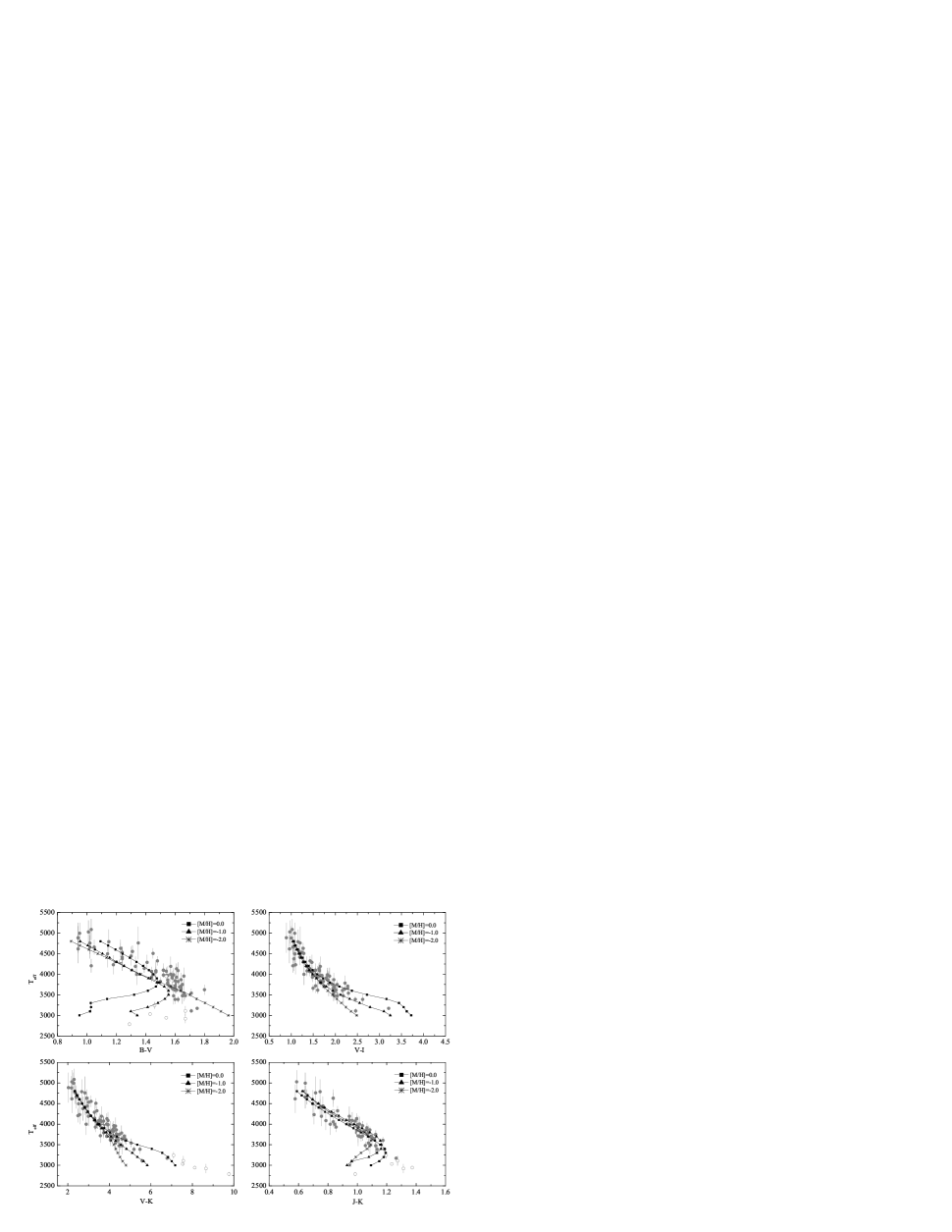
Figure 1: Influence of metallicity on synthetic photometric colors in different $T_{\rm eff}$–color planes. Late-type giants from Paper I are shown as filled and open circles, indicating non-variable and variable stars, respectively (see Paper I for more details; stars are only plotted to indicate the spread in the observed $T_{\rm eff}$–color sequences at Solar metallicity, not for a detailed comparison). Thin lines with symbols are PHOENIX colors at $\log g=1.5$ and different metallicities. Symbols are spaced at every $100$ K.

2.2 MARCS and ATLAS spectra and colors

Complementary to the new PHOENIX colors, we also use synthetic colors calculated with MARCS and ATLAS model atmospheres. MARCS spectra were kindly provided to us by B. Plez (private communication, 2003), ATLAS colors were taken from Castelli & Kurucz (2003). In both cases synthetic spectra were calculated in the approximation of plane-parallel geometry, but employing up-to-date lists of line and molecular opacities (see e.g. Plez 2003; Castelli & Kurucz 2003, for more details).

MARCS broad-band photometric colors were calculated in the Johnson-Cousins-Glass photometric system employing the same procedure as with PHOENIX spectra and using zero points obtained from the PHOENIX spectrum of Vega (Paper I).

3 The influence of metallicity on synthetic photometric colors

It can be anticipated that metallicity has a significant effect on the synthetic photometric colors of late-type giants, as both atomic and molecular opacities of various chemical species have a large influence on the emitted spectrum at the low effective temperatures typical for late-type giants (Paper I). In the following we will focus on the effects due to the variations in overall metallicity, $\left[\mathrm{M}/\mathrm{H}\right]$ (assuming Solar-scaled abundances at $\left[\mathrm{M}/\mathrm{H}\right]<0$); the influence of $\alpha$-element abundances, $\left[\mathrm{\alpha}/\mathrm{Fe}\right]$, will be discussed in a separate paper (Kučinskas et al. 2006, in preparation).

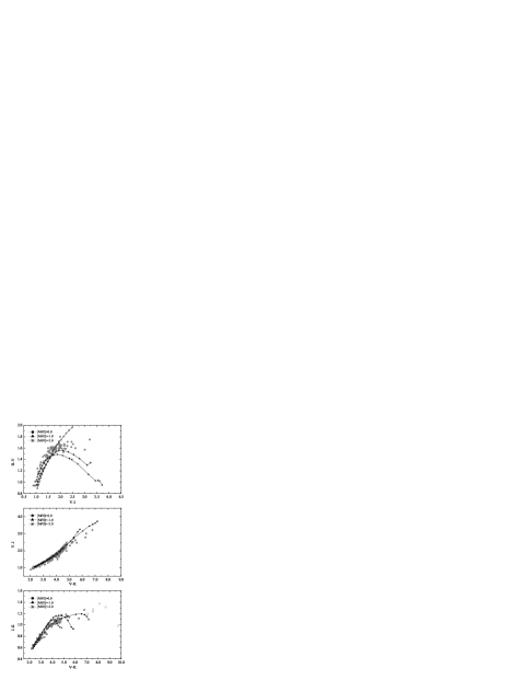
Figure 2: Same as Fig. 1 but in the color–color planes.

The influence of metallicity on the broad-band photometric colors is shown in Fig. 1 ($T_{\rm eff}$–color planes) and Fig. 2 (color–color planes). Together with synthetic colors of PHOENIX at several metallicities ($\left[\mathrm{M}/\mathrm{H}\right]=0,-1.0,-2.0$; $\log g=1.5$), the figures also display observations of individual late-type giants at Solar metallicity from Paper I (with $T_{\rm eff}$ available from interferometry), to illustrate the typical scatter in the observed sequences in $T_{\rm eff}$–color and color–color planes.

Generally, the effects of metallicity are small in all colors of the $T_{\rm eff}$–color planes for $T_{\rm eff}\ga 4000$ K. Most insensitive to the changes in $\left[\mathrm{M}/\mathrm{H}\right]$ is $V-K$, which remains essentially unaffected at $T_{\rm eff}\ga 3700$ K. This behavior simply reflects the fact that photometric colors are little affected by molecular opacities at higher effective temperatures (Paper I), thus the trends in the $T_{\rm eff}$–color planes are governed by changes in atomic opacities which have relatively little influence on the broad-band photometric colors (note that these effects become non-negligible at shorter wavelengths, $\lambda\la 450$ nm).

However, the importance of molecular opacities, and thus the sensitivity to metallicity effects, increases rapidly at lower effective temperatures. This is especially pronounced in the $T_{\rm eff}$–$(B-V)$ plane, where photometric colors develop a strong dependence on metallicity below $T_{\rm eff}\sim 3800$ K (with redder $B-V$ colors at lower $\left[\mathrm{M}/\mathrm{H}\right]$ values in this $T_{\rm eff}$ range; note that the trend is opposite at higher temperatures). The ‘turn-off’ towards the bluer colors (which sets in at $T_{\rm eff}\sim 3800$ K at $\left[\mathrm{M}/\mathrm{H}\right]=0.0$) also tends to occur at lower $T_{\rm eff}$ and redder colors at lower metallicities. As the ‘turn-off’ in the $T_{\rm eff}$–$(B-V)$ plane is caused by the rapidly increasing TiO absorbtion in the $V-$band with decreasing $T_{\rm eff}$ (see Paper I), an increasingly larger fraction of the available Ti is bound in TiO to produce the same band strength at lower $\left[\mathrm{M}/\mathrm{H}\right]$. This causes the ‘turn-off’ to shift to lower effective temperatures with decreasing metallicity, as the efficiency of TiO formation (and thus the concentration of TiO molecules) grows rapidly with decreasing $T_{\rm eff}$.

An increasing influence of metallicity on broad-band photometric colors at lower effective temperatures can be seen in other $T_{\rm eff}$–color planes too, with colors becoming bluer at lower $\left[\mathrm{M}/\mathrm{H}\right]$. Typically, this is due to the decreasing concentration of various molecules at a given effective temperature with decreasing $\left[\mathrm{M}/\mathrm{H}\right]$. For instance, the blueward shift in the $T_{\rm eff}$–$(V-I)$ and $T_{\rm eff}$–$(V-K)$ planes at $T_{\rm eff}\la 4000$ K is essentially governed by the decreasing abundance of TiO at lower $\left[\mathrm{M}/\mathrm{H}\right]$ values (at $T_{\rm eff}\la 3700$ K the effect of lower VO and ${\rm H}_{2}{\rm O}$ concentrations becomes important in $I$ and $K$ bands, respectively). The trends seen in the $T_{\rm eff}$–$(J-K)$ plane are caused by a complex interplay of decreasing concentrations of ${\rm H}_{2}{\rm O}$, CO and TiO (see Paper I for a discussion on the influence of molecular opacities on the photometric colors).

The trends seen in the color–color diagrams essentially reflect the behaviour in the corresponding $T_{\rm eff}$–color planes. The influence of metallicity is strong in the $(B-V)-(V-I)$ plane for $V-I\ga 1.7$; a similar effect is seen in the $(J-K)-(V-K)$ plane for $V-K\ga 4.0$. Note that the effects of metallicity are minor in the $(V-I)-(V-K)$ plane. Interestingly, this color–color plane is also little affected by gravity and the choice of microturbulent velocity (Paper I).

It should be noted that the minimum $T_{\rm eff}$ for which metallicity effects are negligible tends to increase with gravity. For instance, at $\log g=0.5$, the effects of $\left[\mathrm{M}/\mathrm{H}\right]$ in $V-K$ are indeed minor for $T_{\rm eff}\ga 3700$ K, while at $\log g=2.5$ they are only negligible for $T_{\rm eff}\ga 4000$ K. This is due to the fact that at temperatures close to where the molecules dissociate, the effect of metallicity is rather large, as the pressure in the line forming regions increases with lower $\left[\mathrm{M}/\mathrm{H}\right]$ due to the overall lower opacities. This causes a shift in the chemical equilibria in the line forming regions, which is more pronounced at higher gravities (where the relative changes in the pressure are higher) than at low gravities where less molecules form (for given temperature and metallicity).

Table 1: Properties of the Galactic globular cluster sample used in the derivation of $T_{\rm eff}$–$\log g$ relations (see text for details).

Group	Cluster	$n_{star}$	$n_{spec}$	$N$	$\langle\left[\mathrm{Fe}/\mathrm{H}\right]_{\rm CG97}\rangle$	$\langle\left[\mathrm{Fe}/\mathrm{H}\right]_{\rm other}\rangle$	Reference	Age, Gyr
1	M71, NGC 104	21	10	36	$-0.74\pm 0.12$	$-0.81\pm 0.08$	M71: CG97, KI03, R01	M71: $10.2\pm 1.4$
							NGC 104: CG97	NGC 104: $10.7\pm 1.0$
2	M4, M5	31	17	31	$-1.11\pm 0.12$	$-1.17\pm 0.03$	M4: I99	M4: $11.7\pm 0.8$
							M5: CG97	M5: $11.3\pm 1.1$
3	M10, M13,	46	35	70	$-1.40\pm 0.09$	$-1.58\pm 0.09$	M10: KI03	M10: $12.0\pm 1.1$
	NGC 7006						M13: CG97, KI03	M13: $12.5\pm 1.2$
							NGC 7006: KI03	NGC 7006: $13.1\pm 1.0$
4	NGC 6397	10	5	18	$-1.81\pm 0.13$	$-1.98\pm 0.02$	CG97, MPG96	NGC 6397: $12.3\pm 1.1$
5	M15, M92	54	15	66	$-2.16\pm 0.06$	$-2.36\pm 0.05$	M15: KI03, S00	M15: $11.8\pm 0.8$
							M92: CG97, KI03, S00	M92: $12.6\pm 0.9$

4 New $T_{\rm eff}$–$\log g$ scales at $\left[\mathrm{M}/\mathrm{H}\right]<0$

A detailed comparison of synthetic photometric colors with observations in the $T_{\rm eff}$–color planes can be made in a straightforward way if synthetic colors are provided in the form of $T_{\rm eff}$–$\log g$–color relations, with gravities at different temperatures specified according to a representative $T_{\rm eff}$–$\log g$ relation. Such an approach was adopted in Paper I to make a comparison of synthetic and observed colors at Solar metallicity. In this work we employ the same strategy to compare photometric colors of late-type giants at sub-Solar metallicities.

Since a homogeneous set of $T_{\rm eff}$–$\log g$ relations suitable for use with late-type giants at sub-Solar metallicities is not readily available in the literature, we focus in this Section on the derivation of new empirical $T_{\rm eff}$–$\log g$ scales, at $\left[\mathrm{M}/\mathrm{H}\right]=-0.5,-1.0,-1.5,-2.0$. For this purpose we employ a sample of late-type giants in Galactic globular clusters (GGCs), with their effective temperatures and gravities collected from the literature. The choice of GGC giants is based on several considerations. First, GGCs are generally well observed, with precise atmospheric parameters of individual stars available over a wide range of effective temperatures and gravities. Second, GGCs span a wide metallicity range, which is crucial for the derivation of $T_{\rm eff}$–$\log g$ relations at different $\left[\mathrm{M}/\mathrm{H}\right]$. Finally, they are of similar age which implies a similarity in the atmospheric parameters of individual stars in clusters of similar metallicity. This allows binning of stars from different clusters into groups according to their metallicities, to increase the number of individual stars available in a given metallicity group.

4.1 Stellar sample

Ideally, the new $T_{\rm eff}$–$\log g$ relations should be derived using a sample of late-type giants with their effective temperatures and gravities measured using direct methods, e.g., effective temperatures obtained via the interferometric measurements of stellar radii, and gravities from parallaxes (i.e., ‘evolutionary’ gravities, see Sect. 4.1.2 below). Unfortunately, direct measurements of atmospheric parameters are currently available only for the nearby giants, the majority of which have metallicities close to Solar. Needless to say, late-type giants in the GGCs are not accessible, due to the large distances involved. For this reason, our new relations derived in this Section are based on spectroscopic effective temperatures and gravities of GGC giants (in combination with $T_{\rm eff}$ and $\log g$ from photometry, see below), with temperatures obtained under the assumption of excitation equilibrium of Fe I lines, and gravities derived assuming the ionization equilibrium of Fe II lines.

The core of our sample is based on the GGCs analyzed by the Lick-Texas group, in particular, their recent spectroscopic study of late-type giants in 16 GGCs (Kraft & Ivans 2003, KI03, and references therein). Whenever available, data from other sources were also used, providing a consistency check between the results of different groups. We made every attempt to assure that the $T_{\rm eff}$ used in our study are derived from the analysis of recently obtained high quality spectroscopic data, or literature data re-analyzed in a self-consistent and homogeneous way, employing the advantages of improved stellar model atmospheres, analysis techniques, and so forth.

The final sample consists of 82 GGC late-type giants with precise estimates of effective temperatures, gravities and metallicities from high-resolution spectroscopy. Additionally, we use 70 stars with $T_{\rm eff}$ and $\log g$ available from photometry, which nearly doubles the number of stars and individual measurements of stellar parameters available for the analysis. We justify the latter choice by making a careful verification of the effective temperatures and gravities derived with photometry, spectroscopy and the infrared flux method (IRFM; Blackwell et al. 1990), finding a generally good agreement in $T_{\rm eff}$ and $\log g$ obtained with these different methods (Sect. 4.1.1 and Sect. 4.1.2). Metallicities of the individual sample stars are in the range of $\left[\mathrm{Fe}/\mathrm{H}\right]=-0.7\dots-2.5$.

Individual clusters with similar $\left[\mathrm{Fe}/\mathrm{H}\right]$ values were binned into five metallicity groups, to increase the number of stars in each group. In fact, this procedure may smear intrinsic morphological differences in the giant branches of different clusters in the $T_{\rm eff}$–$\log g$ plane. However, as will be shown in Sect. 5, differences between the RGB sequences of individual clusters in the $T_{\rm eff}$–$\log g$ plane are always considerably smaller than the typical errors in the derivations of $T_{\rm eff}$ and $\log g$.

Properties of the five cluster groups are summarized in Table 1. The contents of columns 3–5 are: $n_{\rm star}$ is a total number of stars in a given group for which a total of $N$ (spectroscopic plus photometric) independent derivations of $T_{\rm eff}$ and $\log g$ is available; $n_{\rm spec}$ gives the number of stars with both effective temperatures and gravities available from high-resolution spectroscopy.

Below we focus on the atmospheric parameters of the sample stars in more detail.

4.1.1 Effective temperatures

Approximately half of the individual cluster giants used in this study (77 stars) have effective temperatures available from spectroscopic analysis (i.e., derived under the assumption of excitation equilibrium of Fe I lines). However, spectroscopic estimates are rather sensitive to different model assumptions, details of the analysis procedure, etc. For example, Thévenin & Idiart (1999) have shown that at low metallicities Fe I lines may suffer considerably from overionization, due to the leakage of UV photons into the outer stellar atmosphere because of the lower opacities associated with lower $\left[\mathrm{Fe}/\mathrm{H}\right]$ values. This may indeed have an effect if the effective temperatures are derived under the assumption of excitation equilibrium of Fe I.

For seventeen late-type giants in three clusters from Table 1 (M92, M13, M71), effective temperatures are available both from spectroscopy (KI03) and the infrared flux method, IRFM (Alonso et al. 1999b, A99). Effective temperatures and angular diameters obtained with the IRFM usually agree fairly well with direct estimates available from interferometry and/or lunar occultations, for stars of different luminosity classes and effective temperatures (see, e.g., Nordgren et al. 2001; Blackwell & Lynas-Gray 1998; Alonso et al. 1999a, 2000). A comparison with the IRFM temperatures may thus offer an independent sanity check for the spectroscopically and photometrically derived effective temperatures. This is done in Fig. 3.

Clearly, the differences between $T_{\rm eff}$ from spectroscopy and $T_{\rm IRFM}$ (filled circles in Fig. 3) are small in the cases of M92 and M13; the average offsets are $\Delta T_{\rm eff}\simeq 30$ K and $\Delta T_{\rm eff}\simeq 40$ K, respectively, (i.e., spectroscopic $T_{\rm eff}$ are higher), with RMS residuals of $\simeq 60$ K and $\simeq 70$ K. There is no evidence for any statistically significant systematic trends either. Note, however, that in the case of M13 the average offset is mostly determined by the large offset of a single star at $T_{\rm IRFM}=3790\,K$ ($\Delta T_{\rm eff}\simeq 180$ K), and amounts to only $\Delta T_{\rm eff}\simeq 10$ K if this star is removed from the averaging procedure. A larger offset is seen in case of M71, with spectroscopic temperatures derived by KI03 being higher by $\Delta T_{\rm eff}\simeq 140$ K (RMS residual $\simeq 30$ K).

Figure 3: Comparison of the IRFM temperatures of late-type giants in Galactic globular clusters used in this work, as derived by Alonso et al. (1999b, A99), with $T_{\rm eff}$ obtained from spectroscopy and photometry (cluster groups 5, 3, 1, top-down; the contents and properties of individual cluster groups are given in Table 1). Different symbols indicate original sources from which spectroscopic (filled circles) and photometric (other symbols) effective temperatures were taken. Note that in case of groups 5 and 3 IRFM temperatures are only available for stars in one cluster.

A comparison of photometrically derived effective temperatures of stars in our sample (available for 33 objects) with those obtained with the IRFM shows that photometric $T_{\rm eff}$ generally tend to be slightly higher, with the average offsets of about $85$ K, $90$ K and $55$ K for clusters in groups 5, 3, and 1, respectively (triangles and asterisks in Fig. 3). While the average offset in group 1 is relatively small, the RMS residual is large ($\simeq 150$ K), due to the large offset of the photometric temperatures of individual stars in M71 ($\simeq 150$ K) derived by Carretta & Gratton (1997, CG97).

Interestingly, while KI03 and CG97 stars in M71 are obvious outliers in Fig. 3, they all lie very close to the average $T_{\rm eff}$–$\log g$ sequence in the $T_{\rm eff}$–$\log g$ plane (Sect. 4.2, Fig. 6). At the same time, there are no signs for the discrepancies between the spectroscopic and evolutionary gravities of these stars (Sect. 4.1.2). Also, their gravities agree well with those of stars from other clusters in this metallicity group. Altogether this may indicate that discrepancies seen in Fig. 3 may in fact be due to somewhat lower IRFM temperatures of A99 rather than the systematically higher temperatures of KI03 and CG97.

One should note, however, that the number of stars used in this comparison is small, thus the trends hinted at in Fig. 3 may clearly be influenced (or even governed) by selection effects. KI03, for instance, find a good agreement between spectroscopically obtained effective temperatures and those resulting from photometry for the majority of late-type giants in their study (containing 149 stars). Nevertheless, the differences in $T_{\rm eff}$ of individual stars derived by different authors may provide an idea about the limits of the precision of photometrically derived effective temperatures, reflecting the influence of various systematical effects, discrepancies in $T_{\rm eff}$ predicted by different $T_{\rm eff}$–color relations, and so forth. It is obvious that in many cases these differences are considerably larger than $\sim 100$ K, a value frequently quoted as a typical uncertainty for the photometrically derived effective temperatures, which suggests that errors in the photometrically derived $T_{\rm eff}$ are frequently seriously underestimated (see also discussion in Paper I).

4.1.2 Gravities

Two kinds of gravities are used in spectroscopic abundance analyses. One is ‘evolutionary’ gravity, which is derived through the $T_{\rm eff}$–$L_{\star}$–$M_{\star}$–$\log g$ relation ($L_{\star}$ and $M_{\star}$ are stellar luminosity and mass, respectively), where effective temperature is typically obtained from photometric colors, luminosity from absolute magnitude and bolometric correction, and the mass is implied from evolutionary tracks. The major disadvantage of evolutionary gravities from the point of view of our study is that an estimate of gravity through the $T_{\rm eff}$–$L_{\star}$–$M_{\star}$–$\log g$ relation makes an implicit use of the $T_{\rm eff}$–$\log g$ scale for the derivation of stellar mass. Fortunately, since all clusters in our sample are old (see Sect. 4.1.3), masses of individual stars on their giant branches should be very similar. In such a situation, the $T_{\rm eff}$–$L_{\star}$–$M_{\star}$–$\log g$ relation becomes essentially independent of stellar mass. Evolutionary models predict that for clusters with ages of $10$ and $13$ Gyr (the limits for the clusters in our sample, Sect. 4.1.3) the difference in $\log g$ because of the difference in mass of the RGB stars ($\la 0.1$ $M_{\odot}$) does not exceed $\sim 0.04$ dex (Yi et al. 2001). Thus, the gravity estimate will basically rely only on the estimate of effective temperature and stellar luminosity.

Another type of gravity estimate is obtained directly from the spectral analysis, i.e., derived under the assumption of ionization equilibrium of Fe I and Fe II lines. These are referred to as ‘spectroscopic’ gravities, and in this case no assumptions regarding the $T_{\rm eff}$–$\log g$ scale are made. However, the assumption of ionization equilibrium for Fe I and Fe II in the atmospheres of late-type stars might be a rather poor approximation. As was mentioned in Sect. 4.1.1, Fe I lines (especially in metal-poor stars) may form in conditions that are far from the LTE, due to overionization of Fe I by ultraviolet radiation (Thévenin & Idiart 1999). As a consequence, surface gravities derived under this assumption may also be in error. Nissen et al. (1997) have shown that there indeed exists a systematic discrepancy between spectroscopic gravities and those obtained using HIPPARCOS parallaxes. Unfortunately, the samples discussed by Nissen et al. (1997) do not extend into the gravity range of late-type giants. Only three stars have $\log g<3.0$ in the sample of Thévenin & Idiart (1999), however, the differences between LTE and NLTE gravities for these stars are less than $0.1$ dex.

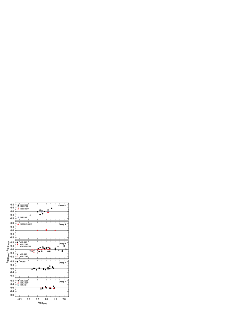
Figure 4: The difference between spectroscopic and evolutionary gravities of Galactic globular cluster giants used in this work, for clusters in groups 5 to 1 in Table 1 (top-down). Spectroscopic gravities are from MPG96 for NGC6397, I99 for M4, and from KI03 for the rest of cluster giants. Different symbols indicate original sources from which evolutionary gravities were taken (see text for details). Note that in case of groups 4, 2, 1 spectroscopic and evolutionary gravities are available for stars in only one cluster.

A detailed comparison of spectroscopic and evolutionary gravities was recently made by KI03 for a large sample of late-type giants in 16 GGCs. They find a good agreement between the two types of gravity estimates within a large range of gravities, effective temperatures and metallicities. Similar conclusions were reached also by Ivans et al. (1999, I99) and Ivans et al. (2001) in their studies of late-type giants in the globular clusters M4 and M5, respectively.

The conclusions of KI03 and I99 are well reflected in Fig. 4, where we compare spectroscopic and evolutionary gravities of stars in the GGCs listed in Table 1. The differences between spectroscopic and evolutionary gravities are calculated using spectroscopic $\log g$ from Minniti et al. (1996, MPG96) for NGC6397, I99 for M4, and KI03 for the rest of cluster giants. Evolutionary gravities were taken from a number of sources (CG97; I99; KI03; Ramirez et al. 2001, R01; Sneden et al. 2000, S00). The agreement between spectroscopic and evolutionary gravities is very good within a large interval of gravities and metallicities, $\log g\sim 0.2\dots 2.2$ and $\left[\mathrm{Fe}/\mathrm{H}\right]\sim-0.7\dots-2.5$, with no indication of statistically significant offsets or systematical trends (Fig. 4). There are no obvious trends between the data of different authors either. Formal linear fits drawn through the data in Fig. 4 do not deviate from $(\log g)_{\rm SPEC}-(\log g)_{\rm EVOL}=0$ by more than $0.2$ dex within the entire interval of gravities and metallicities. The RMS scatter of the data around $\Delta\log g=0$ is largest for stars in cluster group 3 (M10, M13, NGC 7006), $\simeq 0.2$ dex, which is similar to a typical error margin of spectroscopically derived gravities ($\sim 0.2$ dex).

In case of several clusters (M15, M92, M13, NGC 7006) there is an indication that at $\log g\la 0.8$ evolutionary gravities of some stars may be somewhat higher than those obtained from spectroscopy. One possible explanation for this slight discrepancy may be that some of these stars are in fact on the AGB, not the RGB. Since the outer atmospheres may be more extended in case of AGB stars, spectroscopic gravities may indicate lower effective $\log g$ than what would be inferred from the $T_{\rm eff}$–$L_{\star}$–$M_{\star}$–$\log g$ relation.

4.1.3 Metallicities and ages

Figure 5: The difference between metallicities derived by KI03 and those obtained in other studies for the cluster giants used in this work, plotted against $\left[\mathrm{Fe}/\mathrm{H}\right]$ of KI03. Different symbols indicate the original sources from which the $\left[\mathrm{Fe}/\mathrm{H}\right]$ values were taken.

Metallicities of individual stars in groups 1, 3, 5 (Table 1) are compared in Fig. 5, which shows the difference between $\left[\mathrm{Fe}/\mathrm{H}\right]$ estimates obtained by KI03 and those derived by other authors. Whenever available, we used metallicities derived from the Fe II lines, to avoid possible bias due to inadequate treatment of Fe I lines with LTE model atmospheres of late-type giants (cf. Thevenin & Idiart 1999; see also KI03 for a discussion).

There is a clear indication that Fe abundances derived by CG97 are systematically higher than those obtained by KI03, by $\simeq 0.16$ dex on average (with an RMS scatter of $\pm 0.12$ dex). Similarly, $\left[\mathrm{Fe}/\mathrm{H}\right]$ values of CG97 are higher than those derived by MPG96 by $\simeq 0.11$ dex. On the other hand, the data from MPG96 and R01 are in good agreement with the $\left[\mathrm{Fe}/\mathrm{H}\right]$ estimates of KI03. Since the abundances in KI03 seem to agree well with the $\left[\mathrm{Fe}/\mathrm{H}\right]$ scales of Zinn & West (1984), and Rutledge et al. (1997), it is most likely that these differences simply reflect a well known discrepancy between the metallicity scales of Zinn & West (1984) and CG97. We, therefore, derive two average $\left[\mathrm{Fe}/\mathrm{H}\right]$ values for each cluster group: one estimate based on CG97 metallicities, the other on KI03, combined with data from other sources (MPG96, S00, R01). Only in groups 1 and 2 is there a good agreement between the two scales; differences within the other groups are marginally significant (at the $1-2\sigma$ level). It should be mentioned though, that in all cases the spread in metallicities within a particular cluster group is small; typically, $\sim 95\%$ of stars are within a $\pm 0.2$ dex margin from the mean values given in Table 1.

Ages of the individual clusters (taken from Salaris & Weiss 2002) are provided in Table 1 (age estimate for NGC 7006 is from Santos & Piatti 2004). The cluster ages of Salaris & Weiss (2002) were derived from the difference in luminosity of the horizontal branch and the main sequence turn-off point in the cluster color-magnitude diagram, using both CG97 and Zinn & West (1984) metallicity scales. The differences between ages corresponding to the two metallicity scales are small: for all clusters in Table 1 they are well within $\sim 0.5$ Gyr (Salaris & Weiss 2002), thus averaged values are given in Table 1.

All clusters in our sample are old, with individual ages between $\sim 10-13$ Gyr (Table 1). The shift between the RGB isochrones corresponding to these limiting ages is $\Delta T_{\rm eff}<100$ K at $\left[\mathrm{Fe}/\mathrm{H}\right]=-0.7$, and decreases with lower $\left[\mathrm{Fe}/\mathrm{H}\right]$ (Yi et al. 2001). While the age differences may indeed introduce additional scatter in the $T_{\rm eff}$–$\log g$ plane, no clear indication for such spread is seen in the observed sequences of different cluster groups (Fig. 6, Sect. 4.2), most likely because these differences are smeared out by the larger errors in spectroscopically or photometrically derived effective temperatures and/or gravities.

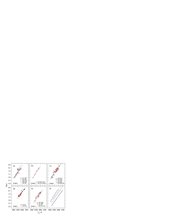
Figure 6:  Empirical $T_{\rm eff}$–$\log g$ relations (solid lines) obtained as best fits to the observed late-type giant sequences in the five cluster groups (Table 1). Panels (a)–(e) show data for groups 5 to 1 respectively; panel (f) displays all derived $T_{\rm eff}$–$\log g$ relations (groups 5 to 1, top-down), together with the $T_{\rm eff}$–$\log g$ scale of Houdashelt et al. (2000, H00) for $\left[\mathrm{Fe}/\mathrm{H}\right]=0.0$ (thick solid line). Different symbols indicate original sources from which the data were taken.

4.2 New $T_{\rm eff}$–$\log g$ scales

The gravities of individual stars in all five cluster groups (Table 1) are plotted versus the effective temperature in Fig. 6. Generally, there is good consistency in $T_{\rm eff}$ and $\log g$ of individual giants within a particular cluster group (even though these stars belong to different clusters), especially in groups 2, 4, and 5. Several stars at $T_{\rm eff}\sim 4500$ K in M15 (group 5, Fig. 6a) are somewhat off the main trend, as their spectroscopic gravities are considerably lower than those of other stars in this effective temperature range; similarly deviating is one star in M92 at $T_{\rm eff}\sim 4200$ K. It should be reminded that spectroscopic $\log g$ of these stars are about $0.4$ dex lower than their evolutionary gravities (see Fig. 4). Note however, that the resulting $T_{\rm eff}$–$\log g$ scale for this cluster group remains essentially unaffected if these stars are not employed in its derivation. Slightly larger scatter is seen in group 3, though data from different sources seem to agree well, with no noticeable differences or trends between them. With the exception of the CG97 data for NGC 104, there is also a good consistency in the effective temperatures and gravities of individual stars in group 1.

There is a faint hint that the sequence of CG97 stars in M92 is slightly shifted towards lower effective temperatures with respect to the best fitting sequence containing all stars in group 5. A similar offset is more clearly seen for the CG97 data in NGC 104 (group 1), where effective temperatures of CG97 are lower by about $\sim 150$ K. Fortunately, in both cases these offsets have minor impact on the resulting $T_{\rm eff}$–$\log g$ scales (which are not altered significantly if these stars are excluded), and we therefore retain them in the further analysis.

The new empirical $T_{\rm eff}$–$\log g$ relations obtained as best fits to the observed giant sequences in the five cluster groups (Table 1) are shown in Fig. 6 and are provided in numerical form in Tables 2 and 3 (Table 3 lists coefficients of polynomial fits representing the new relations). The typical RMS residual of the best fit is $\simeq 0.15$ dex in $\log g$ (see Table 2), which corresponds to about $\simeq 100$ K in $T_{\rm eff}$ (note that the typical uncertainties in spectroscopically and/or photometrically derived $T_{\rm eff}$ and $\log g$ are somewhat larger, $\sim 150$ K and $\sim 0.3$ dex, respectively). This uncertainty (RMS residual) is slightly smaller than the typical errors in the $T_{\rm eff}$–color relations of A99 that are based on stellar temperatures derived with the IRFM (up to $\sim 150$ K), and the RMS residuals of the $T_{\rm eff}$–color relations based on the effective temperatures from interferometry ($\sim 160$ K, Paper I).

Table 2: Empirical $T_{\rm eff}$–$\log g$ relations for the late-type giants in different cluster groups, obtained as best fits to the data in Fig. 6. Column 2 gives $\log g$ according to the $T_{\rm eff}$–$\log g$ scale of Houdashelt et al. (2000, H00) linearly extrapolated to $T_{\rm eff}=4800$ K. The last line is RMS residual of the best-fit, expressed as a gravity difference.

$T_{\rm eff}$	log g
	$\left[\mathrm{Fe}/\mathrm{H}\right]$=0.0	Gr 1	Gr 2	Gr 3	Gr 4	Gr 5
4900	–	–	–	2.29	2.21	2.00
4800	2.90	2.46	–	2.05	1.95	1.77
4700	2.69	2.23	–	1.82	1.70	1.55
4600	2.49	2.01	1.78	1.60	1.47	1.33
4500	2.28	1.80	1.58	1.38	1.24	1.11
4400	2.08	1.59	1.38	1.17	1.02	0.91
4300	1.89	1.39	1.19	0.97	0.82	0.70
4200	1.69	1.19	1.00	0.77	0.62	0.51
4100	1.50	1.01	0.82	0.58	0.44	0.31
4000	1.30	0.82	0.65	0.40	0.27	0.13
3900	1.11	0.65	0.48	0.23	–	–
3800	0.93	0.48	0.31	0.06	–	–
3700	0.74	0.31	0.16	-0.10	–	–
3600	0.57	–	0.01	-0.25	–	–
3500	0.39	–	–	–	–	–
3400	0.21	–	–	–	–	–
3300	0.04	–	–	–	–	–
RMS residual:		0.18	0.12	0.15	0.06	0.16

Table 3: Analytical expressions corresponding to the empirical $T_{\rm eff}$–$\log g$ relations given in Table 2, in the form $\log g=a_{0}+a_{1}T_{\rm eff}+a_{2}T_{\rm eff}^{2}+a_{3}T_{\rm eff}^{3}+a_{4}T_{\rm eff}^{4}$.

Group	$a_{0}$	$a_{1}$	$a_{2}$	$a_{3}$	$a_{4}$	$T_{\rm eff}$ range, K
$\left[\mathrm{Fe}/\mathrm{H}\right]=0.0$	8.07	–1.045e-2	3.997e-6	–5.814e-10	3.240e-14	$3300\leq T_{\rm eff}\leq 4800$
1	–1.41	–6.761e-4	3.086e-7	–	–	$3700\leq T_{\rm eff}\leq 4800$
2	–1.51	–6.394e-4	2.948e-7	–	–	$3600\leq T_{\rm eff}\leq 4600$
3	–0.95	–1.100e-3	3.597e-7	–	–	$3600\leq T_{\rm eff}\leq 4900$
4	2.60	–2.820e-3	5.596e-7	–	–	$4000\leq T_{\rm eff}\leq 4900$
5	–2.87	–3.360e-4	2.714e-7	–	–	$4000\leq T_{\rm eff}\leq 4900$

Table 4: New $T_{\rm eff}$–$\log g$ relations at several metallicities, obtained by interpolating empirical $T_{\rm eff}$–$\log g$ relations from Table 2. The new relations are given for the metallicity scales of KI03 and CG97 (see text for details).

$T_{\rm eff}$	log g
		$\left[\mathrm{Fe}/\mathrm{H}\right]$ according to						$\left[\mathrm{Fe}/\mathrm{H}\right]$ according to
		CG97 metallicity scale						KI03 metallicity scale
		–0.5	–1.0	–1.5	–2.0			–0.5	–1.0	–1.5	–2.0
4900		2.80	2.52	2.28	2.09			2.83	2.59	2.37	2.15
4800		2.58	2.29	2.04	1.85			2.61	2.35	2.13	1.90
4700		2.36	2.06	1.81	1.61			2.39	2.12	1.89	1.67
4600		2.14	1.84	1.59	1.38			2.17	1.90	1.67	1.44
4500		1.93	1.63	1.37	1.17			1.96	1.68	1.45	1.22
4400		1.73	1.42	1.16	0.95			1.76	1.48	1.24	1.01
4300		1.53	1.22	0.96	0.75			1.56	1.28	1.04	0.81
4200		1.34	1.03	0.76	0.56			1.37	1.08	0.84	0.61
4100		1.15	0.84	0.57	0.37			1.18	0.90	0.65	0.43
4000		0.97	0.66	0.39	0.19			1.00	0.72	0.47	0.25
3900		0.80	0.49	0.21	0.02			0.82	0.55	0.30	0.08
3800		0.63	0.33	0.04	–0.15			0.65	0.38	0.13	–0.08
3700		0.46	0.17	–0.12	–0.30			0.48	0.23	–0.03	–0.23
3600		0.30	0.02	–0.28	–0.45			0.32	0.08	–0.18	–0.37
3500		0.15	–0.13	–0.42	–0.59			0.17	–0.07	–0.32	–0.51

We also provide $T_{\rm eff}$–$\log g$ relations at several additional metallicities corresponding to the metallicity nodes in the PHOENIX, MARCS and ATLAS grids of synthetic photometric colors, at $\left[\mathrm{M}/\mathrm{H}\right]=-0.5,-1.0,-1.5,-2.0$. These supplementary relations were obtained by quadratic interpolation between the empirical $T_{\rm eff}$–$\log g$ relations in cluster groups 1-5 (Tables 2 and 3). The empirical relations were extrapolated to cover the range $T_{\rm eff}=3500\dots 4900$ K before making the interpolation. Note, however, that in most cases extrapolation was only done by up to 100 K in $T_{\rm eff}$, which corresponds to $\sim 0.2$ dex in $\log g$. Exceptions are relations in groups 4 and 5 ($\left[\mathrm{Fe}/\mathrm{H}\right]<-1.8$), which were extrapolated to lower effective temperatures by as much as 500 K, and thus should be used with caution below $T_{\rm eff}\sim 3900$ K. Metallicities for the individual cluster groups were assigned according to the metallicity scales of CG97 and KI03, thus two sets of interpolated $T_{\rm eff}$–$\log g$ relations corresponding to each metallicity scale are provided (Table 4). Table 5 gives analytical expressions corresponding to the new $T_{\rm eff}$–$\log g$ relations provided in Table 4. It should be noted that differences between the $T_{\rm eff}$–$\log g$ relations corresponding to the two metallicity scales are always less than $0.1$ dex in $\log g$ (or, correspondingly, $\sim 50$ K in $T_{\rm eff}$, see Fig. 7). The RMS residuals of the interpolation procedure do not exceed $0.03$ dex in $\log g$.

Figure 7: The difference in gravities predicted by the new $T_{\rm eff}$–$\log g$ relations (Table 4) based on the metallicity scales of KI03 and CG97, at several $\left[\mathrm{Fe}/\mathrm{H}\right]$.

Table 5: Analytical expressions corresponding to the new $T_{\rm eff}$–$\log g$ relations given in Table 4, in the form $\log g=a_{0}+a_{1}T_{\rm eff}+a_{2}T_{\rm eff}^{2}$.

$\left[\mathrm{Fe}/\mathrm{H}\right]$	$a_{0}$	$a_{1}$	$a_{2}$
CG97 scale
-0.5	–1.85	–3.761e-4	2.703e-7
-1.0	–0.82	–1.010e-3	3.453e-7
-1.5	–1.41	–8.991e-4	3.371e-7
-2.0	–0.48	–1.420e-3	3.969e-7
KI03 scale
-0.5	–1.81	–3.885e-4	2.726e-7
-1.0	–0.52	–1.130e-3	3.600e-7
-1.5	–0.78	–1.150e-3	3.657e-7
-2.0	0.09	–1.650e-3	4.225e-7

Table 6: $T_{\rm eff}$–$\log g$–color relations for the late-type giants based on the synthetic colors calculated with PHOENIX and MARCS model atmospheres. Photometric colors are given in the Johnson-Cousins-Glass system (see Sect. 2 for details).

			PHOENIX				MARCS
$T_{\rm eff}$	$\log g$		$B\!-\!V$	$V\!-\!I$	$V\!-\!K$	$J\!-\!K$	$B\!-\!V$	$V\!-\!I$	$V\!-\!K$	$J\!-\!K$
			$\left[\mathrm{Fe}/\mathrm{H}\right]$=–0.5
4900	2.83		0.931	0.994	2.226	0.596	–	–	–	–
4800	2.61		0.977	1.033	2.328	0.626	–	–	–	–
4700	2.39		1.023	1.075	2.437	0.658	–	–	–	–
4600	2.17		1.076	1.121	2.553	0.693	–	–	–	–
4500	1.96		1.130	1.170	2.677	0.729	1.157	1.138	2.662	0.735
4400	1.76		1.190	1.227	2.813	0.768	1.218	1.190	2.792	0.774
4300	1.56		1.250	1.288	2.958	0.810	1.279	1.245	2.932	0.816
4200	1.37		1.317	1.357	3.118	0.855	1.347	1.312	3.086	0.860
4100	1.17		1.385	1.435	3.291	0.903	1.420	1.387	3.255	0.907
4000	1.00		1.452	1.523	3.479	0.953	1.492	1.472	3.439	0.957
3900	0.82		1.525	1.630	3.692	1.004	1.562	1.570	3.644	1.009
3800	0.65		1.592	1.757	3.932	1.058	1.624	1.690	3.876	1.065
3700	0.48		1.650	1.915	4.212	1.114	1.672	1.841	4.148	1.121
3600	0.32		1.687	2.136	4.566	1.164	1.691	2.046	4.484	1.179
3500	0.17		1.681	2.436	5.021	1.212	–	–	–	–
			$\left[\mathrm{Fe}/\mathrm{H}\right]$=–1.0
4900	2.59		0.880	0.986	2.230	0.605	–	–	–	–
4800	2.35		0.926	1.025	2.329	0.635	–	–	–	–
4700	2.12		0.975	1.067	2.438	0.667	–	–	–	–
4600	1.90		1.031	1.113	2.554	0.702	–	–	–	–
4500	1.68		1.094	1.165	2.681	0.738	1.114	1.135	2.661	0.739
4400	1.48		1.157	1.220	2.816	0.778	1.183	1.185	2.783	0.774
4300	1.28		1.229	1.284	2.966	0.820	1.249	1.247	2.933	0.819
4200	1.08		1.304	1.355	3.128	0.866	1.330	1.312	3.080	0.858
4100	0.90		1.384	1.433	3.302	0.914	1.402	1.387	3.255	0.910
4000	0.72		1.471	1.523	3.498	0.966	1.484	1.466	3.429	0.956
3900	0.55		1.560	1.622	3.707	1.021	1.561	1.559	3.638	1.018
3800	0.38		1.659	1.744	3.945	1.078	1.641	1.663	3.851	1.071
3700	0.23		1.753	1.886	4.211	1.137	–	–	–	–
3600	0.08		1.832	2.068	4.520	1.191	–	–	–	–
3500	–0.07		1.883	2.320	4.910	1.239	–	–	–	–
			$\left[\mathrm{Fe}/\mathrm{H}\right]$=–1.5
4900	2.37		0.846	0.992	2.234	0.606	–	–	–	–
4800	2.13		0.896	1.031	2.335	0.635	–	–	–	–
4700	1.89		0.952	1.074	2.443	0.667	–	–	–	–
4600	1.67		1.014	1.123	2.561	0.701	–	–	–	–
4500	1.45		1.084	1.177	2.691	0.737	1.091	1.147	2.674	0.741
4400	1.24		1.164	1.241	2.832	0.775	1.170	1.207	2.810	0.778
4300	1.04		1.248	1.310	2.987	0.817	1.252	1.273	2.957	0.819
4200	0.84		1.342	1.390	3.159	0.860	1.338	1.343	3.117	0.863
4100	0.65		1.440	1.479	3.351	0.910	1.425	1.418	3.289	0.911
4000	0.47		1.543	1.579	3.557	0.963	1.514	1.501	3.475	0.964
3900	0.30		1.656	1.695	3.789	1.018	1.606	1.592	3.680	1.022
3800	0.13		1.774	1.824	4.043	1.078	–	–	–	–
3700	–0.03		1.896	1.968	4.316	1.139	–	–	–	–
3600	–0.18		2.017	2.150	4.631	1.196	–	–	–	–
3500	–0.32		1.998	2.243	4.941	1.319	–	–	–	–
			$\left[\mathrm{Fe}/\mathrm{H}\right]$=–2.0
4900	2.15		0.820	1.002	2.240	0.604	–	–	–	–
4800	1.90		0.878	1.046	2.341	0.632	–	–	–	–
4700	1.67		0.944	1.094	2.453	0.662	–	–	–	–
4600	1.44		1.018	1.148	2.574	0.692	–	–	–	–
4500	1.22		1.107	1.214	2.711	0.725	1.094	1.183	2.706	0.738
4400	1.01		1.200	1.285	2.858	0.759	1.186	1.253	2.849	0.773
4300	0.81		1.304	1.370	3.029	0.798	1.282	1.327	3.006	0.813
4200	0.61		1.417	1.465	3.218	0.842	1.382	1.406	3.175	0.857
4100	0.43		1.534	1.571	3.426	0.889	1.484	1.490	3.358	0.906
4000	0.25		1.660	1.696	3.664	0.939	1.588	1.580	3.555	0.961
3900	0.08		1.787	1.828	3.918	0.994	–	–	–	–
3800	–0.08		1.917	1.981	4.212	1.059	–	–	–	–
3700	–0.23		2.050	2.150	4.524	1.121	–	–	–	–
3600	–0.37		2.178	2.328	4.843	1.181	–	–	–	–
3500	–0.51		2.207	2.568	5.140	1.175	–	–	–	–

It is worth remarking that the clusters in our sample are old; thus the masses of their RGB stars should be low, typically $\sim 0.8-0.9$ $M_{\odot}$ (Yi et al. 2001). Though the direct effect of stellar mass on the broad-band photometric colors is small (see Paper I), $T_{\rm eff}$–$\log g$ relations will indeed be different in case of younger stellar populations, because of the higher masses of their RGB stars. For example, at $\left[\mathrm{M}/\mathrm{H}\right]=-1.0$ and $T_{\rm eff}=4400$ K, the gravity on the 2 Gyr isochrone will be about 0.15 dex lower than $\log g$ corresponding to the same effective temperature on the 15 Gyr isochrone (this difference is smaller at lower $T_{\rm eff}$ and $\left[\mathrm{M}/\mathrm{H}\right]$, Yi et al. 2001). Fortunately, the effect of this difference is small: a shift in gravity by $\sim 0.15$ dex at $T_{\rm eff}=4400$ K will translate to $\Delta(B-V)\sim 0.02$ for $\left[\mathrm{Fe}/\mathrm{H}\right]=-1.0$ and to $\sim 0.03$ for $\left[\mathrm{Fe}/\mathrm{H}\right]=-2.0$, with colors at lower $\log g$ becoming redder (differences in other colors are smaller).

While the new $T_{\rm eff}$–$\log g$ relations provided in Tables 4 and 5 cover the effective temperature range of $T_{\rm eff}=3500-4900$ K, it should be taken into account that uncertainties in these relations will likely be larger below $T_{\rm eff}\sim 3900$ K and above $T_{\rm eff}\sim 4600$ K, where an extrapolation was used to compensate for a lack of stars in certain cluster groups. It should also be noted that the new $T_{\rm eff}$–$\log g$ relations provided in Tables 2 and 4 are representative for RGB stars. Appropriate care should thus be taken if these relations are used at higher (or lower) temperatures, where RGB stars may be mixed up with stars on the horizontal branch (or AGB stars).

5 Synthetic photometric colors versus observations: results and discussion

The new $T_{\rm eff}$–$\log g$ relations that were discussed in the previous Section allow us to derive a set of new $T_{\rm eff}$–$\log g$–color relations based on the synthetic photometric colors, and to compare them with various $T_{\rm eff}$–color and color–color relations available from the literature. This comparison is done separately for $\left[\mathrm{M}/\mathrm{H}\right]=-1.0$ and $-2.0$. Below we focus on the details of these steps.

5.1 New $T_{\rm eff}$–$\log g$–color scales

The new $T_{\rm eff}$–$\log g$–color relations were constructed using the $T_{\rm eff}$–$\log g$ relations derived in Sect. 4.2 and broad-band photometric colors calculated with the PHOENIX, MARCS, and ATLAS stellar model atmospheres (Sect. 2). These relations are provided in Table 6 (scales employing PHOENIX and MARCS colors) and Table 7 (relation based on ATLAS colors). They are based on the new empirical $T_{\rm eff}$–$\log g$ scales corresponding to the metallicity scale of KI03 (Sect. 4.2), and are delivered at four metallicities, $\left[\mathrm{M}/\mathrm{H}\right]=-0.5$, $-1.0$, $-1.5$, and $-2.0$. Note that the limiting gravities in MARCS and ATLAS grids of synthetic colors are $\log g=0.5$ and $\log g=0.0$, respectively; to extend the coverage in $\log g$, MARCS and ATLAS colors were linearly extrapolated to $\sim 0.2$ dex below these values.

Uncertainties in the new $T_{\rm eff}$–$\log g$–color relations are governed by the uncertainties in the empirical $T_{\rm eff}$–$\log g$ scales that were obtained as best fits to the observed $T_{\rm eff}$–$\log g$ sequences of late-type giants in Galactic globular clusters (Sect. 4.2). The typical RMS residual of the fitting procedure is $\simeq 0.15$ dex in $\log g$, or $\simeq 100$ K in $T_{\rm eff}$. At $T_{\rm eff}=4400$ K, $\log g=1.5$, and $\left[\mathrm{M}/\mathrm{H}\right]=-1.0$, the uncertainty $\Delta T_{\rm eff}=100$ K will be equivalent to changes in photometric colors $\Delta(B-V)\simeq\Delta(V-I)\simeq 0.05$, $\Delta(V-K)\simeq 0.13$, and $\Delta(J-K)\simeq 0.04$ (correspondingly, to 0.07, 0.05, 0.14, and 0.04 mag, at $\log g=1.0$ and $\left[\mathrm{M}/\mathrm{H}\right]=-2.0$). The effect on photometric colors will increase slightly with decreasing gravity. Note, however, that photometric colors are less sensitive to uncertainties in $\log g$: at $T_{\rm eff}=4400$ K, $\log g=1.5$, and $\left[\mathrm{M}/\mathrm{H}\right]=-1.0$, $\Delta\log g=0.15$ will correspond to $\Delta(B-V)\simeq 0.02$, with differences in other colors at the level of 0.01 mag or lower. While we will further quote $\pm 100$ K as a representative uncertainty of the new $T_{\rm eff}$–$\log g$–color relations, it is rather obvious that this may only represent a lower limit on the true uncertainties, which include various systematical effects inherent in the spectroscopic derivations of $T_{\rm eff}$, $\log g$, and $\left[\mathrm{Fe}/\mathrm{H}\right]$, limitations of the current stellar atmosphere models, and so forth.

Table 7: $T_{\rm eff}$–$\log g$–color relations for the late-type giants based on the synthetic colors calculated with ATLAS model atmospheres. Photometric colors are given in the Johnson-Cousins-Glass system (see Sect. 2 for details).

			ATLAS
$T_{\rm eff}$	$\log g$		$B\!-\!V$	$V\!-\!I$	$V\!-\!K$	$J\!-\!K$
$\left[\mathrm{Fe}/\mathrm{H}\right]$=–0.5
4750	2.50		1.010	1.033	2.383	0.660
4500	1.96		1.133	1.141	2.671	0.751
4250	1.47		1.273	1.275	3.013	0.857
4000	1.00		1.453	1.465	3.438	0.974
3750	0.56		1.657	1.739	3.975	1.098
3500	0.17		1.811	2.176	4.695	1.196
$\left[\mathrm{Fe}/\mathrm{H}\right]$=–1.0
4750	2.24		0.959	1.030	2.386	0.666
4500	1.68		1.098	1.142	2.673	0.755
4250	1.18		1.259	1.283	3.019	0.859
4000	0.72		1.465	1.478	3.453	0.978
3750	0.31		1.708	1.747	3.989	1.107
3500	–0.07		1.946	2.109	4.606	1.206
$\left[\mathrm{Fe}/\mathrm{H}\right]$=–1.5
4750	2.01		0.926	1.037	2.395	0.668
4500	1.45		1.089	1.161	2.688	0.753
4250	0.94		1.285	1.322	3.051	0.853
4000	0.47		1.532	1.542	3.512	0.971
3750	0.05		1.813	1.839	4.090	1.104
3500	–0.32		–	–	–	–
$\left[\mathrm{Fe}/\mathrm{H}\right]$=–2.0
4750	1.79		0.900	1.052	2.408	0.667
4500	1.22		1.099	1.198	2.715	0.745
4250	0.71		1.344	1.397	3.111	0.838
4000	0.25		1.636	1.666	3.625	0.952
3750	–0.16		–	–	–	–
3500	–0.51		–	–	–	–

5.2 Comparison of $T_{\rm eff}$–color and color–color relations

In principle, the new $T_{\rm eff}$–$\log g$–color relations can be readily used to compare synthetic photometric colors with observed effective temperatures and colors of late-type giants in the $T_{\rm eff}$–color planes. Such an approach was taken in Paper I, where for this purpose we used a sample of late-type giants with effective temperatures derived from interferometric measurements of stellar radii. Unfortunately, as was already mentioned in Sect. 4.1, effective temperatures of late-type giants obtained from interferometry or lunar occultations are very scarce at sub-Solar metallicities. The sample of late-type giants in Galactic globular clusters which was employed in the previous Section to obtain the new $T_{\rm eff}$–$\log g$ relations can not be used for this purpose either, since the number of stars in each metallicity group is too small for a reliable comparison of observed and synthetic photometric colors in different $T_{\rm eff}$–color planes at different metallicities.

Instead of using effective temperatures and photometric colors of individual stars we thus will make a comparison of synthetic photometric colors with the $T_{\rm eff}$–color and color–color relations available from the literature. For this purpose we use relations based both on the observed and theoretical colors of late-type giants, at $\left[\mathrm{M}/\mathrm{H}\right]=-1.0$ and $-2.0$.

The baseline set of $T_{\rm eff}$–color and color–color relations used in our comparisons is that of Alonso et al. (1999b, A99). These relations are built on the observed properties of a homogenous sample of 250 late-type giants in Galactic globular clusters, with precise optical and near-infrared photometry of individual stars and $T_{\rm eff}$ from IRFM. The sample covers the metallicity range $\left[\mathrm{Fe}/\mathrm{H}\right]=0\dots-3.0$, with $\left[\mathrm{Fe}/\mathrm{H}\right]$ estimates obtained either from spectroscopy or Strömgren photometry (with typical accuracies of $\pm 0.15$ dex and $0.2$ to $0.3$ dex, respectively). The IRFM temperatures of individual stars are typically in good agreement with those obtained by direct methods within a large range of effective temperatures ($T_{\rm eff}\sim 3700\dots 5200$ K). The mean difference between the interferometric and IRFM temperatures is $T_{\rm direct}-T_{\rm IRFM}=3\pm 51$ K, based on 20 stars (Alonso et al. 1999a). The internal accuracy of the individual $T_{\rm eff}$–color relations varies between $40$ and $125$ K, which compares well with the accuracies of the $T_{\rm eff}$–color scales derived by us in Paper I employing a sample of stars with interferometric temperatures (which are of the order of $\pm 150$ K). Before making the comparisons, the $T_{\rm eff}$–color relations of A99 (Table 6 of A99, Johnson system) were transformed to the standard Johnson-Cousins-Glass system (Sect. 2), using transformation equations from Fernie (1983) for $(V-I)$, and from Bessell & Brett (1988) for $(V-K)$ and $(J-K)$.

Recently, the $T_{\rm eff}$–color and color–color relations of A99 were updated by Ramírez & Meléndez (2005a, b). We include these new relations into our analysis, too. The transformation of Ramírez & Meléndez (2005b, RM05) colors involving the 2MASS bandpasses ($V-K_{2}$, $J_{2}-K_{2}$; subscript 2 denotes the 2MASS system) to the standard Johnson-Cousins-Glass system was made using transformation equations given by Carpenter (2001).

Several additional widely used $T_{\rm eff}$–color and color–color relations that were employed in our study are:

• Bell & Gustafsson (1989, BG89): $T_{\rm eff}$–color and color–color relations based on theoretical photometric colors. The BG89 scales employed in this study were constructed using $B-V$ colors taken from Bell & Gustafsson (1978), $V-I$, $V-K$, and $J-K$ colors from Bell & Gustafsson (1989). According to Vandenberg & Clem (2003), the scale of BG89 reproduces well the observed CMDs of Galactic open and globular clusters at different metallicities. In the effective temperature range of interest for this study, the agreement seems to be very good, both at $\left[\mathrm{M}/\mathrm{H}\right]=-1.0$ and $-2.0$ (Vandenberg & Clem 2003);

• BaSeL 2.2 (Lejeune et al. 1998, BaSeL 2.2): a semiempirical library of photometric colors based on the theoretical spectra. While photometric colors of BaSeL 2.2 are calibrated to match empirical $T_{\rm eff}$–color relations at $\left[\mathrm{Fe}/\mathrm{H}\right]=0.0$, with presumably poorer consistency at lower metallicities, we employ this scale in the present study too, partially to compare it with the BaSeL 3.1 colors (see below). BaSeL 2.2 colors used in this work were calculated using the interactive web-based BaSeL server;

• BaSeL 3.1 (Westera et al. 2002, BaSeL 3.1): extension of the BaSeL 2.2 library to lower metallicities, calibrated using the photometric data of Galactic globular clusters. This scale is designed to reproduce the $T_{\rm eff}$–color and color-color relations at metallicities down to $\left[\mathrm{M}/\mathrm{H}\right]\sim-2.0$. BaSeL 3.1 colors used in this study were calculated using the web-based BaSeL server;

• Houdashelt et al. (2000, H00): synthetic colors based on theoretical spectra calculated with the MARCS and SSG codes, with TiO opacities adjusted to reproduce the observed spectra of M giants from Fluks et al. (1994). The H00 scale should be used with care below $T_{\rm eff}\sim 3800$ K since no ${\rm H_{2}O}$ opacities were included in the calculations (see Paper I for more details on the influence of different molecular opacities on the photometric colors);

• Sekiguchi & Fukugita (2000, SF00): an empirical $T_{\rm eff}$–$(B-V)$ scale based on the observed colors and effective temperatures of 537 Infrared Space Observatory (ISO) standard stars from Di Benedetto (1998). Effective temperatures of individual stars were derived from the $T_{\rm eff}$–$(V-K)$ relation, calibrated on a sample of nearby stars with angular diameters available from interferometry;

• Vandenberg & Clem (2003, VC03): empirical scales based on synthetic BVRI colors of Bell & Gustafsson (1978, 1989), adjusted to satisfy observational constrains from the observed CMDs of Galactic globular and open clusters, field stars in the Solar neighborhood, empirical $T_{\rm eff}$–color relations and color–color relations for field giants.

Note that in all cases photometric colors were selected according to the new $T_{\rm eff}$–$\log g$ relations derived in Sect. 4.2.

Extensive comparisons of these relations with various other $T_{\rm eff}$–color scales have been published in numerous studies (e.g., Alonso et al. 1999b; Houdashelt et al. 2000; Sekiguchi & Fukugita 2000; Westera et al. 2002; Vandenberg & Clem 2003; Ramírez & Meléndez 2005b). Some of these relations (BaSeL 2.2, A99, H00, SF00, and VC03) were also employed in our comparison of the observed and theoretical colors of late-type giants at Solar metallicity (Paper I). Altogether, this provides a further reference list for a comparison of the new $T_{\rm eff}$–color and color–color scales with similar relations available in the literature.

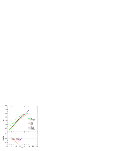
Figure 11: (a) Top: Empirical and theoretical color–color relations at $\left[\mathrm{Fe}/\mathrm{H}\right]=-2.0$, in the $(B-V)-(V-I)$ plane. The thick solid line is the $(B-V)-(V-I)$ relation of A99, the thick dashed line is empirical $T_{\rm eff}$–color relation at Solar metallicity (Paper I). Several existing $T_{\rm eff}$–color relations are shown, together with the scales constructed using synthetic colors of PHOENIX, MARCS and ATLAS. Bottom: the difference between various $(B-V)-(V-I)$ relations and the A99 scale, $\Delta{\rm CI}={\rm CI}^{other}-{\rm CI}^{A99}$.

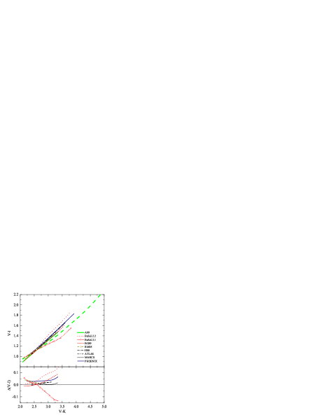
Figure 11: (b) Same as in Fig. 11a but in the $(V-I)-(V-K)$ plane.

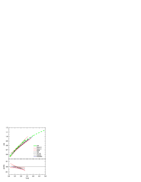
Figure 11: (c) Same as in Fig. 11a but in the $(J-K)-(V-K)$ plane.

Comparisons of the new $T_{\rm eff}$–$\log g$–color relations based on PHOENIX, MARCS and ATLAS colors (Tables 6 and 7) with the published $T_{\rm eff}$–color relations are given in Fig. 8 ($T_{\rm eff}$–color planes) and Fig. 9 (color–color planes) at $\left[\mathrm{M}/\mathrm{H}\right]=-1.0$, and, correspondingly, in Figs. 10 and 11 at $\left[\mathrm{M}/\mathrm{H}\right]=-2.0$ (all comparisons are made with respect to the scale of A99). We discuss the trends at these two metalicities in the sections below.

5.2.1 $\left[\mathrm{M}/\mathrm{H}\right]=-1.0$

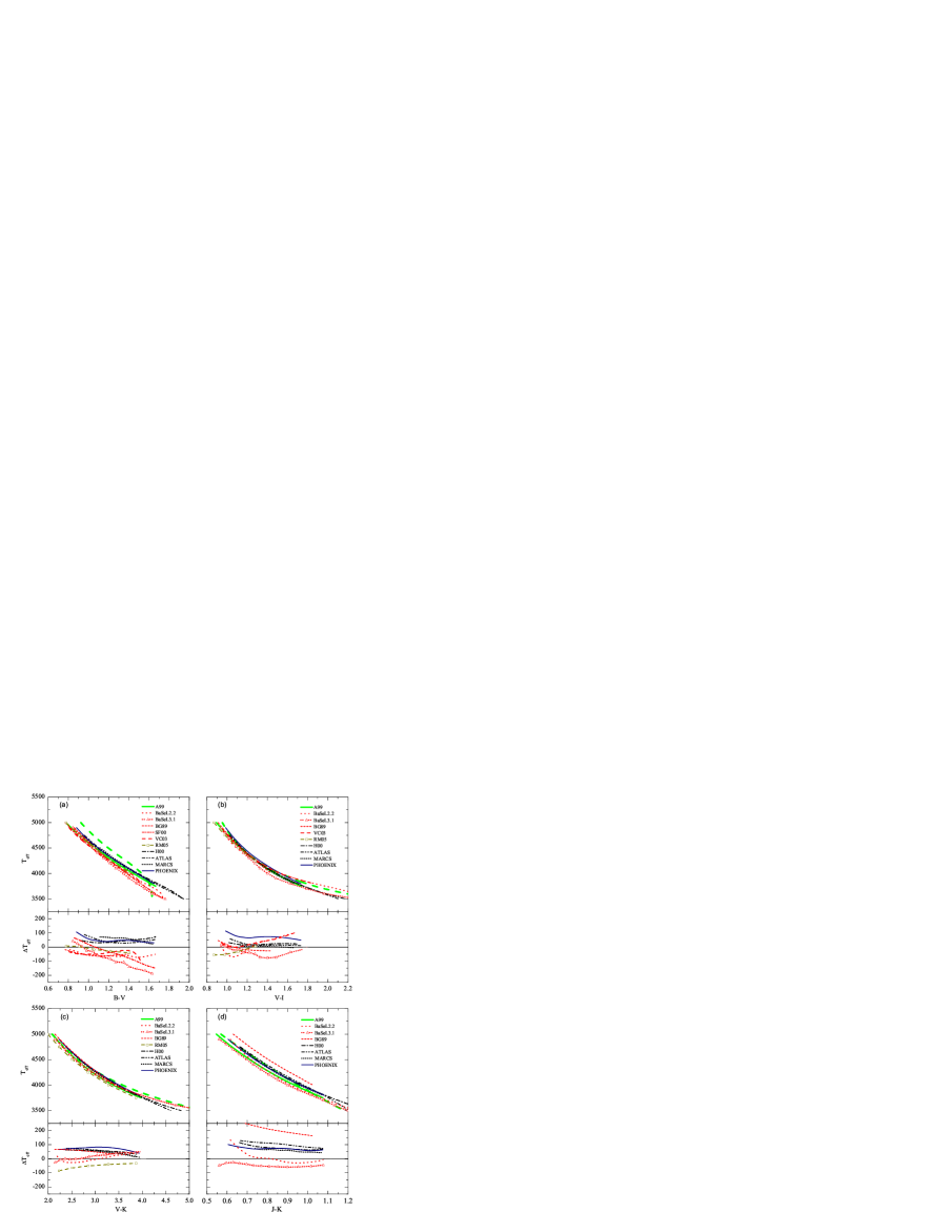
Figure 8: Empirical and theoretical $T_{\rm eff}$–color relations for late-type giants at $\left[\mathrm{M}/\mathrm{H}\right]=-1.0$, in different $T_{\rm eff}$–color planes (a-d, top panels). The thick solid line shows $T_{\rm eff}$–color relation of A99, the thick dashed line is the empirical $T_{\rm eff}$–color relation at Solar metallicity (Paper I). Several existing $T_{\rm eff}$–color relations are shown as well, together with the scales constructed using synthetic colors of PHOENIX, MARCS and ATLAS (Tables 6 and 7). The bottom panels in each figure show the difference between various $T_{\rm eff}$–color relations and the A99 scale in a given $T_{\rm eff}$–color plane ($\Delta T_{\rm eff}=T_{\rm eff}^{other}-T_{\rm eff}^{A99}$.)

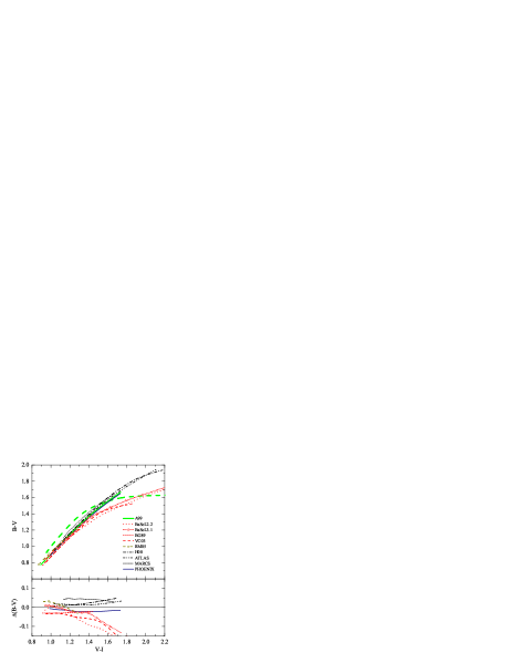
Figure 9: (a) Top: Empirical and theoretical color–color relations at $\left[\mathrm{M}/\mathrm{H}\right]=-1.0$ in the $(B-V)-(V-I)$ plane. The thick solid line is the $(B-V)-(V-I)$ relation of A99, the thick dashed line is the empirical $T_{\rm eff}$–color relation at Solar metallicity (Paper I). Several existing $T_{\rm eff}$–color relations are shown, together with the scales constructed using synthetic colors of PHOENIX, MARCS and ATLAS. Bottom: the difference between various $(B-V)-(V-I)$ relations and the A99 scale, $\Delta{\rm CI}={\rm CI}^{other}-{\rm CI}^{A99}$.

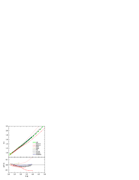
Figure 9: (b) Same as in Fig. 9a but in the $(V-I)-(V-K)$ plane.

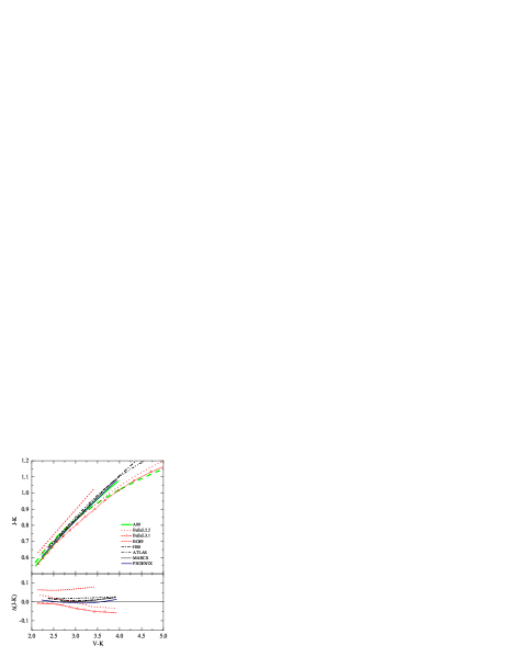
Figure 9: (c) Same as in Fig. 9a but in the $(J-K)-(V-K)$ plane.

On the whole, the agreement between different $T_{\rm eff}$–color relations is good in all $T_{\rm eff}$–color planes (Fig. 8). Typical differences are well within $\Delta T_{\rm eff}\sim 80$ K, with somewhat larger deviations in the $T_{\rm eff}$–$(J-K)$ plane. Except for the scales of SF00 and BaSeL 3.1 (which start to deviate below $T_{\rm eff}\sim 4100$ K and $\sim 4300$ K, correspondingly), reasonably good agreement is also seen in the $T_{\rm eff}$–$(B-V)$ plane (note that effective temperature–color relations differ considerably more in this plane at Solar metallicity; see Paper I). It is worthwhile noting that the slopes of SF00 and BaSeL 3.1 scales are clearly different from those of other relations in this $T_{\rm eff}$–color plane. The agreement between different relations is very good in the $T_{\rm eff}$–$(V-I)$ plane, typically to $\pm 50$ K, with somewhat larger deviations for the scales based on BaSeL and PHOENIX colors. There is also a good consistency between different $T_{\rm eff}$–color scales in the $T_{\rm eff}$–$(V-K)$ plane (to $\pm 80$ K), though effective temperatures predicted by the $T_{\rm eff}$–color relation of A99 are slightly lower than those resulting from other relations.

In spite of the reasonably good agreement between the different $T_{\rm eff}$–color scales in general, there is a clear indication that effective temperatures predicted by the $T_{\rm eff}$–color relations based on synthetic colors (H00, ATLAS, MARCS, PHOENIX) are typically slightly higher than those inferred from the empirical relations (i.e., those of A99, BaSeL 2.2 and 3.1, SF00, VC03, RM05). This offset is seen in all $T_{\rm eff}$–color planes and is largest in the $T_{\rm eff}$–$(B-V)$ plane, where the average difference between the predictions of theoretical and empirical relations amounts to $\sim 100$ K (similar offset is seen in the $T_{\rm eff}$–$(J-K)$ plane too, though in this case the comparison can only be made with the semi-empirical BaSel 2.2 and 3.1 scales). The only exception in this sense is the scale of BG89: theoretical colors of BG89 are very similar to those predicted by empirical relations in the $T_{\rm eff}$–$(B-V)$ and $T_{\rm eff}$–$(V-I)$ planes. In the $T_{\rm eff}$–$(V-K)$ plane, the BG89 relation is similar to the other scales based on synthetic colors, while in the $T_{\rm eff}$–$(J-K)$ plane it predicts effective temperatures that are considerably higher than those resulting from other $T_{\rm eff}$–color relations.

It should be noted that the A99 scale occupies an intermediate position in this sense in all $T_{\rm eff}$–color planes, providing a compromise between the predictions of theoretical and empirical $T_{\rm eff}$–color relations. That is, effective temperatures given by the A99 scale generally tend to be lower than those given by $T_{\rm eff}$–color relations based on synthetic colors, with an average offset of about $\sim 60$ K. On the other hand, they are higher by up to $\sim 50$ K ($T_{\rm eff}$–$(B-V)$ plane) than effective temperatures predicted by the empirical scales. Ivans et al. (2001) have reached similar conclusions in their comparison of the effective temperatures of RGB stars in the globular cluster M5 derived using the $T_{\rm eff}$–$(B-V)$ scales of A99, SF00 and H00. While there are some hints that the A99 scale tends to predict slightly lower $T_{\rm eff}$ than other $T_{\rm eff}$–color relations at Solar metallicity (Paper I), at $\left[\mathrm{M}/\mathrm{H}\right]=-1.0$ a similar trend is seen only in the $T_{\rm eff}$–$(V-K)$ plane (it is interesting to note in this respect that the $T_{\rm eff}$’s predicted by A99 scales at $\left[\mathrm{M}/\mathrm{H}\right]=-2.0$ are indeed lower than those resulting from other $T_{\rm eff}$–color relations; see Sect. 5.2.2).

While the RM05 scale (which is an extension and update of the A99 relations) predicts slightly different effective temperatures than do the A99 relations, differences between the two scales are always within $\pm 50$ K. A slightly larger discrepancy is seen in the $T_{\rm eff}$–$(V-K)$ plane, especially at $T_{\rm eff}\ga 4300$ K. Note, however, that the transformation equations of Carpenter (2001) used by us to convert $(V-K)_{\rm 2MASS}$ colors of RM05 to the Johnson-Cousins-Glass system (see Sect. 2 for details) were derived utilizing only a part of the 2MASS survey data available at that time. Nevertheless, a shift of $\Delta(V-K)=0.1$ is needed to compensate for a difference of $50$ K between the A99 and RM05 relations (Fig. 8c), which is quite large to be explained by uncertainties in the transformation equations.

We find no clear evidence that the $T_{\rm eff}$–color relations based on the BaSeL 3.1 colors would indeed represent an improvement over the BaSeL 2.2 scales at $\left[\mathrm{M}/\mathrm{H}\right]=-1.0$. In fact, the scales employing BaSeL 2.2 colors seem to be in better agreement with the general trends seen in the $T_{\rm eff}$–$(B-V)$ and $T_{\rm eff}$–$(V-I)$ planes at $T_{\rm eff}\la 4500$ K. Otherwise, the two scales behave very similarly, especially in the $T_{\rm eff}$–$(V-K)$ and $T_{\rm eff}$–$(J-K)$ planes (though differences gradually start to build up in the latter case at $T_{\rm eff}>4500$ K).

The agreement between synthetic colors calculated using different stellar atmosphere models is very good (including the scale based on H00 colors), with differences typically well within $\Delta T_{\rm eff}\sim 70$ K. A somewhat larger discrepancies are seen in the $T_{\rm eff}$–$(V-I)$ plane, where the $T_{\rm eff}$–color scale based on the PHOENIX colors tends to predict somewhat higher effective temperatures than those resulting from other $T_{\rm eff}$–color relations (a similar trend is seen at Solar metallicity, see Paper I).

The $T_{\rm eff}$–color relations of BG89 are based on theoretical colors that were calculated nearly 20 years ago (Bell & Gustafsson 1978, 1989). This offers an intriguing possibility for examining the changes/improvements made in the theoretical modeling of stellar spectra and photometric colors over the last two decades, by comparing the predictions of BG89 with the new $T_{\rm eff}$–color relations based on colors calculated with the current state-of-the-art stellar model atmospheres (i.e., PHOENIX, MARCS, and ATLAS). Interestingly, very little difference is seen between the two sets of theoretical $T_{\rm eff}$–color relations in the $T_{\rm eff}$–$(V-I)$ and $T_{\rm eff}$–$(V-K)$ planes. This is remarkable, especially since the $V$, $I$, and $K$ passbands are strongly influenced by various molecular bands (TiO, VO, ${\rm H}_{2}{\rm O}$, etc.). The differences are larger in the $T_{\rm eff}$–$(B-V)$ and $T_{\rm eff}$–$(J-K)$ planes though. Compared with the effective temperatures obtained using $T_{\rm eff}$–color relations based on the synthetic colors of PHOENIX, MARCS, and ATLAS, the $T_{\rm eff}$ predicted by the BG89 scale are approximately $\sim 100$ K lower in the former case and by a similar amount higher in the latter. On the whole, the differences in photometric colors provided by BG89 and those calculated with the current stellar model atmospheres are not large, typically $\la 100$ K.

The agreement between different color–color relations is good in all color–color planes (Fig. 9). The differences are well within $\sim\pm 0.05$ mag in the $(B-V)$–$(V-I)$ plane, while the agreement is even better in the $(V-I)$–$(V-K)$ and $(J-K)$–$(V-K)$ planes (to $\sim\pm 0.03$ mag). Note, however, that the scales based on BaSeL 2.2. and 3.1 colors are rather deviant in all color–color planes at the redder colors (below $T_{\rm eff}\sim 4000-4300$ K). Similarly, the VC03 relation starts to deviate beyond $V-I\simeq 1.5$ in the $(B-V)$–$(V-I)$ plane. BG89 colors are discrepant in the $(J-K)$–$(V-K)$ plane (due to deviations in the $T_{\rm eff}$–$(J-K)$ plane), within the entire range of photometric colors (or effective temperatures) typical for late-type giants.

5.2.2 $\left[\mathrm{M}/\mathrm{H}\right]=-2.0$

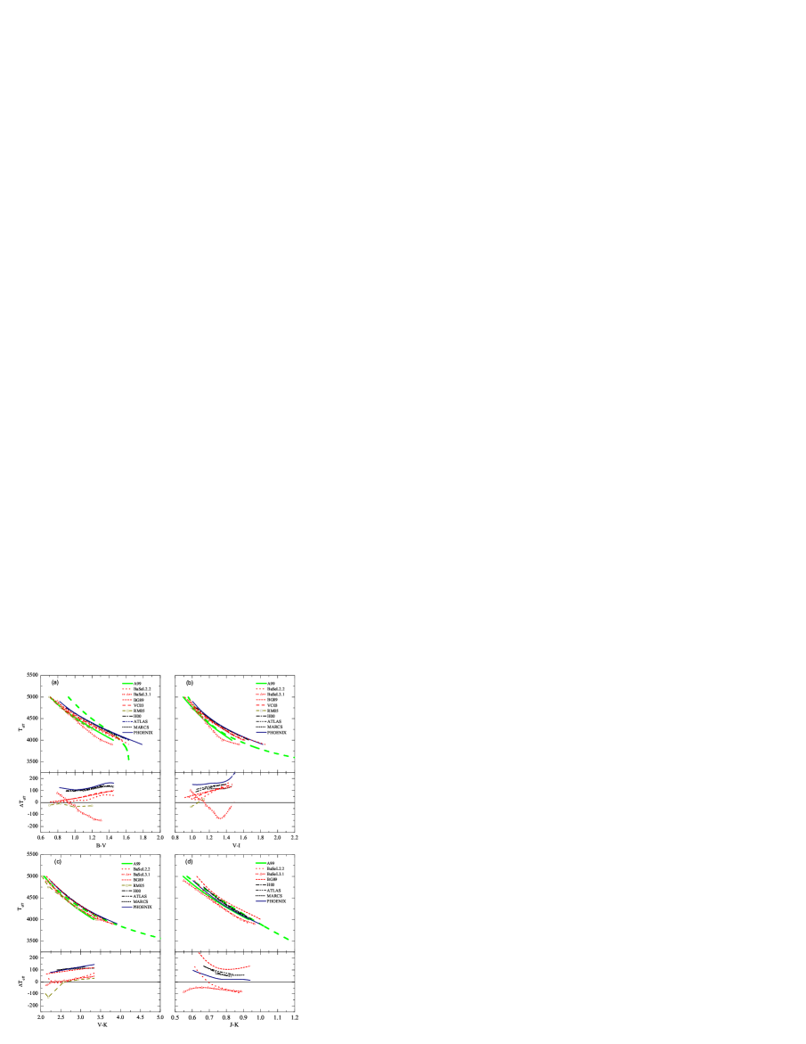
Figure 10: Empirical and theoretical $T_{\rm eff}$–color relations at $\left[\mathrm{Fe}/\mathrm{H}\right]=-2.0$, in different $T_{\rm eff}$–color planes (a-d, top panels). The thick solid line is the $T_{\rm eff}$–color relation of A99, the thick dashed line is empirical $T_{\rm eff}$–color relation at Solar metallicity (Paper I). Several existing $T_{\rm eff}$–color relations are shown as well, together with the scales constructed using synthetic colors of PHOENIX, MARCS and ATLAS (Tables 6 and 7). The bottom panels in each figure show the difference between various $T_{\rm eff}$–color relations and the A99 scale in a given $T_{\rm eff}$–color plane ($\Delta T_{\rm eff}=T_{\rm eff}^{other}-T_{\rm eff}^{A99}$.)

Obviously, the agreement between various $T_{\rm eff}$–color relations and the scale of A99 is poorer at $\left[\mathrm{Fe}/\mathrm{H}\right]=-2.0$ (Fig. 10). Effective temperatures predicted by the A99 scales are systematically lower than those resulting from the other $T_{\rm eff}$–color relations, by up to $\sim 150$ K. This tendency is clearly seen in all $T_{\rm eff}$–color planes, and applies to scales based both on observed and theoretical colors (though the discrepancies are typically larger in the latter case, to $\sim 130$ K on average). It should be noted, however, that A99 relations are in reasonable agreement with other empirical relations in the $T_{\rm eff}$–$(B-V)$ and $T_{\rm eff}$–$(V-K)$ planes (to $\sim 90$ K and $\sim 70K$, respectively); larger deviations occur only when A99 relations are compared with those employing theoretical colors. Whether these inadequacies point out to deficiencies in the A99 calibrations, or problems with the predictions of theoretical models (or both) - this has to be clarified in the future studies.

The agreement between $T_{\rm eff}$–color scales based on different sets of synthetic colors is very good, with deviations typically within $\Delta T_{\rm eff}\sim 40$ K. This is not an unexpected result, since differences in the setup of stellar atmosphere models (opacities, equation of state, etc.) generally become less important at lower metallicities as their effect on the resulting model structures becomes smaller too. Scales based on PHOENIX colors are slightly more discrepant in the $T_{\rm eff}$–$(V-I)$ and $T_{\rm eff}$–$(J-K)$ planes, though in the latter case this results in a better agreement with the A99 scale. The $T_{\rm eff}$–color relations based on BG89 colors are very similar to those employing theoretical colors calculated with current PHOENIX, MARCS, and ATLAS stellar model atmospheres. Significant differences are seen only in the $T_{\rm eff}$–$(B-V)$ plane, where effective temperatures predicted by the BG89 relations are cooler by about $\sim 100$ K, and in the $T_{\rm eff}$–$(J-K)$ plane, where BG89 scales predict effective temperatures that are systematically higher than those resulting from the other scales based on synthetic colors.

Similarly to what was seen at $\left[\mathrm{M}/\mathrm{H}\right]=-1.0$, we find no clear evidence that scales employing BaSeL 3.1 colors would indeed perform better than those based on BaSeL 2.2. In fact, BaSeL 2.2 colors are in much better agreement with the general trends seen in the $T_{\rm eff}$–$(B-V)$ and $T_{\rm eff}$–$(V-I)$ planes, both with respect to the scale of A99 and other $T_{\rm eff}$–color relations. On the contrary, BaSeL 3.1 scales deviate rapidly below $T_{\rm eff}\sim 4600$ K in the $T_{\rm eff}$–$(B-V)$ and $T_{\rm eff}$–$(V-I)$ planes, predicting effective temperatures that are too low. The two sets of relations are nearly identical in the $T_{\rm eff}$–$(V-K)$ plane, with slightly larger differences seen in the $T_{\rm eff}$–$(J-K)$ plane at $T_{\rm eff}\ga 4500$ K.

The new scales of RM05 behave very similarly to those of A99. The differences are always within $\sim\pm 40$ K, except that RM05 temperatures in the $T_{\rm eff}$–$(V-K)$ plane are up to $\sim 120$ K lower than those predicted by empirical scales at $\ga 4500$ K, and to $\sim 200$ K lower than those resulting from the relations based on theoretical colors.

The agreement between different scales in the color–color planes is generally very good. The differences are typically well within $\sim\pm 0.03$ mag (except for scales based on BaSeL colors), with a marginally larger scatter seen in the $(J-K)$–$(V-K)$ plane, $\sim\pm 0.05$ mag. The only outliers are scales based on BaSeL 2.2 and 3.1 colors, as they deviate rapidly in the $(B-V)$–$(V-I)$ and $(V-I)$–$(V-K)$ planes beyond $(V-I)\simeq 1.2$ and $(V-K)\simeq 2.6$.

Indeed, most of the $T_{\rm eff}$–color scales employed in this comparison are sensitive to the $T_{\rm eff}$–$\log g$ relations used in their derivation. However, uncertainties in the $T_{\rm eff}$–$\log g$ relations cannot fully account for the size of systematic offsets seen above, e.g., those between the A99 relations and other $T_{\rm eff}$–color scales, as these differences are simply too large. Theoretical models predict that at a given photometric color higher effective temperatures will correspond to the models with lower gravities. Our comparison shows that effective temperatures inferred from the different $T_{\rm eff}$–color relations are indeed always higher than those resulting from the A99 scales. Obviously, such differences may result if gravities predicted by the new $T_{\rm eff}$–$\log g$ relations are systematically too low. However, in order to account for the average offset of $\sim 100$ K seen in the $T_{\rm eff}$–$(V-I)$ and $T_{\rm eff}$–$(V-K)$ planes, gravities in the $T_{\rm eff}$–$\log g$ relations should be increased correspondingly by about 0.5 and 1 dex at $\left[\mathrm{M}/\mathrm{H}\right]=-2.0$ (generally, larger changes will be needed at higher metallicities). A shift of $\sim 0.4$ dex in gravity will be required to remedy the situation in the $T_{\rm eff}$–$(B-V)$ plane. Clearly, the required shifts in gravity are too large to offer a plausible solution in this situation, especially given the fact that the gravity difference between the empirical $T_{\rm eff}$–$\log g$ relations (Sect. 4.2) at $\left[\mathrm{M}/\mathrm{H}\right]=-1.0$ and $-2.0$ is only about $\sim 0.5$ dex.

6 Conclusions

A detailed investigation of the metallicity effects on the broad-band photometric colors of late-type giants shows that their photometric properties are generally little affected by the variations in $\left[\mathrm{M}/\mathrm{H}\right]$ at effective temperatures higher than $T_{\rm eff}\sim 3800$ K. This picture gradually changes at lower $T_{\rm eff}$, as the influence of metallicity becomes more strongly pronounced below $T_{\rm eff}<3500$ K. To a large extent this is due to changing efficiency of molecule formation with decreasing $\left[\mathrm{M}/\mathrm{H}\right]$: since spectra of the late-type giants are heavily blanketed by molecular lines (especially at low $T_{\rm eff}$), photometric colors are inevitably affected when molecular lines become weaker at lower $\left[\mathrm{M}/\mathrm{H}\right]$.

In order to compare synthetic colors with observations of late-type giants, we derive a set of new $T_{\rm eff}$–$\log g$–color scales based on spectroscopic and photometric effective temperatures and gravities of 152 late-type giants in 10 Galactic globular clusters, backed up with synthetic colors produced with PHOENIX, MARCS and ATLAS stellar model atmospheres. We find that the new scales employing synthetic colors agree well with various existing $T_{\rm eff}$–color relations at $\left[\mathrm{M}/\mathrm{H}\right]=-1.0$, with typical differences being well within $\Delta T_{\rm eff}\sim 100$ K. However, effective temperatures predicted by the theoretical scales tend to be higher than those resulting from the empirical relations, by up to $\sim 100$ K. Similar trends are seen at $\left[\mathrm{M}/\mathrm{H}\right]=-2.0$ too, especially in the $T_{\rm eff}$–$(B-V)$ and $T_{\rm eff}$–$(V-K)$ planes, where $T_{\rm eff}$ inferred from the empirical relations are again by about $\sim 100$ K lower than those predicted by the theoretical scales.

The agreement between the different color–color relations is good in all color–color planes, both at $\left[\mathrm{M}/\mathrm{H}\right]=-1.0$ and $\left[\mathrm{M}/\mathrm{H}\right]=-2.0$. The typical differences are within $\pm 0.05$ mag, although in certain color–color planes the agreement is even better, to $\pm 0.03$ mag (e.g., in the $(B-V)$–$(V-I)$ and $(V-I)$–$(V-K)$ planes, both at $\left[\mathrm{M}/\mathrm{H}\right]=-1.0$ and $-2.0$).

Finally, there is a good consistency in synthetic colors calculated with different stellar model atmospheres in $T_{\rm eff}$–color and color–color planes, both at $\left[\mathrm{M}/\mathrm{H}\right]=-1.0$ and $\left[\mathrm{M}/\mathrm{H}\right]=-2.0$. The typical differences are within $\Delta T_{\rm eff}\sim 70$ K at $\left[\mathrm{M}/\mathrm{H}\right]=-1.0$ and $\Delta T_{\rm eff}\sim 40$ K at $\left[\mathrm{M}/\mathrm{H}\right]=-2.0$ in $T_{\rm eff}$–color planes, and within $\Delta\sim 0.07$ mag at both metallicities in all color–color planes. Let us note, however, that the differences in the setup of stellar atmosphere models (opacities, equation of state, etc) generally become less important at low metallicities which leads to a better agreement between colors calculated with different model atmospheres (the differences in photometric colors are considerably larger at Solar metallicity; see Paper I).