A New Method to Calibrate the Magnitudes of Type Ia Supernovae at Maximum Light

Abstract

We present a new empirical method for fitting multicolor light curves of Type Ia supernovae. Our method combines elements from two widely used techniques in the literature: the $\Delta$m₁₅ template fitting method (Phillips et al., 1999) and the Multicolor Light-Curve Shape method (MLCS; Riess, Press, & Kirshner, 1996). An advantage of our technique is the ease of adding new colors, templates, or parameters to the fitting procedure. We use a large sample of published light curves to calibrate the relations between the absolute magnitudes at maximum and the post-maximum decline rate $\Delta{\rm m}_{15}$ in $BVRI$ filters. If we perform a cut in reddening and compare an unreddened with a reddened sample, we find that the two samples produce relations which are marginally consistent with each other. We find that individual subsamples from a given survey or publication have significantly tighter relationships between light curve shape and luminosity than the relationship derived from the sum of all the samples, pointing to uncorrected systematic errors in the photometry, mainly in $BV$ filters. Using our method, we calculate luminosity distances and host galaxy reddening to 89 SNe in the Hubble flow and construct a low-$z$ Hubble diagram. The dispersion of the SNe in the Hubble diagram is $\sigma=0.20$ mag, or an error of $\sim 9\%$ in distance to a single SN. Our technique produces similar or smaller dispersion in the low-$z$ Hubble diagram than other techniques in the literature.

1 Introduction

Type Ia supernovae (Type Ia SNe), the thermonuclear explosions of accreting white dwarfs (Arnett, 1982), are the most precise distance indicators at cosmological distances. Even though they are not standard candles (Pskovskii, 1977; Branch, 1987; Phillips, 1993), their absolute magnitudes at maximum light are closely correlated with the shape of their light curves (Phillips, 1993). As precise standardizable candles they have been used to trace the expansion of the Universe as a function of redshift (see Leibundgut, 2000), leading to the discovery of the acceleration of the expansion (Riess et al., 1998; Perlmutter et al., 1999), and the transition from deceleration at early times to acceleration in the present (Tonry et al., 2003; Riess et al., 2004).

All the information of the luminosity distance of a Type Ia SN is in the multicolor light curves. Different empirical methods have been presented in the literature to fit Type Ia SNe light curves (LCs). Among the most developed are: $\Delta$m₁₅, MLCS, and the “stretch” method.

The $\Delta$m₁₅ method (Hamuy et al., 1996a; Phillips et al., 1999) uses six $BVI$ templates of nearby SNe (Hamuy et al., 1996d) covering a wide range of light curve shapes which are parametrized by a single discrete value: the 15 day post-maximum decline in magnitude in the $B$ band $\Delta$m${}_{15}(B)$. Germany et al. (2004) provided a modified version of the method by including the $R$ band in the fits, new estimations of the $K$-corrections, and new templates from well-observed nearby SNe.

In the MLCS method (Riess, Press, & Kirshner, 1996; Riess et al., 1998) a continuous parameter characterizes different light curve shapes. This parameter is the difference between the absolute magnitude at maximum of a SN and a fiducial value, constructed from a set of well observed SNe. The latest version of the method (Jha, Riess, & Kirshner, 2006b) has added the $U$ filter to $BVRI$ and better extinction estimators.

The stretch method (Perlmutter et al., 1997; Goldhaber et al., 2001) measures the light curve shape by simply adjusting the scale on the time axis by a multiplicative factor. This is an elegant solution, since the stretch of the light curve is the combination of the cosmological redshift effect ($1+z$ factor) and the intrinsic light curve shape. Different LCs are stretched in the time domain to fit a template (Leibundgut, 1988). This method has been used mainly in $UBV$ filters because of the homologous nature of the light curves across all light curve shapes. $\Delta$m₁₅ and MLCS are more robust to non-homologous variations as a function of light curve shape in the redder filters.

Other methods have been proposed (Tripp, 1998; Tripp & Branch, 1999; Tonry et al., 2003; Wang et al., 2003, 2005). Wang et al. (2005) found a tight correlation between peak luminosities and the intrinsic colors at $\sim$12 days after $B$ maximum. Using this correlation but with a small sample of SNe, they obtain very low-dispersion Hubble diagrams.

The new technique presented in this paper is a combination of $\Delta$m₁₅ and MLCS methods. We implement what we consider the advantages from each method: the direct use of actual (not interpolated) SNe LCs templates characterized by different $\Delta$m₁₅ values in the fitting method, and a proper statistical model of the errors in the fitting parameters. We use a simple mathematical framework to account for the non-uniform distribution in the values of the $\Delta$m₁₅ parameter. Our method allows us to calculate a covariance matrix for the fits as in MLCS. It also allows us to trivially add any new supernova light curve or any new color as a template in $\Delta{\rm m}_{15}$ without having to perform a training set calculation.

This paper is organized as follows: in Section 2 we present the template set, composed by 14 templates with different decline rates; in Section 3 we explain the mathematical technique to interpolate between templates and the model to fit the multicolor light curves of SNe; in Section 4 we obtain linear relations between the absolute magnitudes at maximum and $\Delta{\rm m}_{15}$ in rest frame $BVRI$ filters studying a large sample of SNe; in Section 5 we construct a Hubble diagram with a large sample of low-$z$ Type Ia SNe in the Hubble flow, and compare our method with other results published in the literature; and finally, the general conclusions of the results obtained in the paper are presented in Section 6.

2 Light curve templates

The template set, listed in Table A New Method to Calibrate the Magnitudes of Type Ia Supernovae at Maximum Light is composed of the 6 $BVI$ templates of Hamuy et al. (1996d) augmented with the $R$ filter templates of Hamuy et al. (1996d), and 8 new $BVRI$ templates constructed from published and unpublished data of well observed nearby Type Ia SNe. The SNe were selected to cover a wide range in observed light curve shapes. We recalculated the $\Delta{\rm m}_{15}$ from a the spline interpolation of the $B$-band data.

We used the same recipe of Hamuy et al. (1996d) to construct the LC templates. A cubic spline interpolation was applied to the data obtaining the time and magnitude at maximum in each filter, with typical uncertainties of $\sim 0.2-0.5$ days and $\sim 0.02-0.05$ mag, respectively. The time axis in all the filters was parametrized by the rest frame time relative to $B$ maximum. In the cases where the redshift in the Cosmic Mircowave Background (CMB) frame is $z_{CMB}\geq 0.01$, the time axis was corrected for cosmological time dilation dividing by $1+z$, and the magnitudes were $K$-corrected to the rest frame.

We calculated the $K$-corrections in $BVRI$ filters using the recipe of Hamuy et al. (1993) and a set of spectrophotometry from different epochs and SNe: SN 1972E (catalog ), SN 1990N (catalog ), SN 1991T (catalog ), SN 1991bg (catalog ), SN 1992A (catalog ), and SN 1994D (catalog ). We fitted the results with a cubic spline to provide values of $K$-corrections in different epochs, with a typical error $\sim 0.02$ mag.

Finally, the magnitudes at $B$ maximum were subtracted in all the filters to have $B=V=R=I=0.0$ at t${}_{0}(B)$. The final templates have interpolated rest frame magnitudes in the range $-5\leq{\rm t-t}_{0}(B){\rm[days]}\leq 80$, with a sampling of one day.

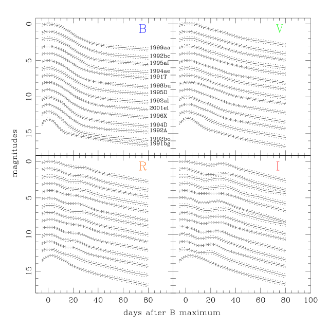
Figure 1: Light curve template set in $BVRI$ filters. These 14 templates, 6 from Hamuy et al. (1996d) and 8 constructed from well sampled light curves, expand a large range in post-maximum decline rates: $0.83\leq\Delta{\rm m}_{15}(B)\leq 1.93$. The dashed lines are the $\pm$1$\sigma$ limits using the interpolated photometric uncertainties as a function of time. We have applied a progressive offset of 1 mag for plotting purposes.

In Table A New Method to Calibrate the Magnitudes of Type Ia Supernovae at Maximum Light we present basic information of the templates and the references of the photometric data. All the LC templates are plotted in Figure 1, ordered by increasing values of $\Delta$m${}_{15}(B)$ from slow decliners to fast decliners. From Figure 1 we can observe the main characteristics of the $BVRI$ light curves: a principal maximum, followed by a change in the curvature of the light curve $\sim 10-30$ days after maximum and a linear decay at greater than $30-40$ days. The $RI$ light curves also have a secondary hump fainter than the first peak at $\sim 20-30$ days. A small inflection in the $V$ light curve can be seen during the same epoch as the $I$ secondary maximum. Different morphological properties of the light curves, such as the time of the secondary peak in the $RI$ filters and the time of inflection, are correlated with the post-maximum decline rate (Hamuy et al., 1996d). The rise times in the $BV$ filters are generally correlated with the post-maximum decline rate (Riess et al., 1999b), slow risers are slow decliners, and fast risers are fast decliners.

The dashed lines around each solid curve in Figure 1 represents the approximate $\pm 1\sigma$ statistical uncertainties in the photometry. These curves were obtained doing a linear interpolation of the errors in the original data points. Typical uncertainties in the photometry from photon statistics and errors in the standards are $\sim 0.02$ mag around maximum and $\geq 0.04$ mag at late times. Note though that the systematic errors that arise from doing photometry on a nebular (as opposed to stellar) spectral energy distribution of late-time SNe are much larger, at the $\sim 0.1$ mag level (Suntzeff, 2000).

3 The method

The principal idea of the method is a formalism which allows us to construct a linear combination of the discrete template set, composed by the observed templates, into a template parametrized by $\Delta$m₁₅. The $\Delta$m₁₅ parameter can then be included in the $\chi^{2}$ function when fitting a new multicolor light curve, allowing us to calculate a covariance matrix and the estimation of statistical uncertainties in the best fitting parameters.

3.1 Interpolation between light curve templates

We interpolate between different templates using a weighting function. It assigns different weights to each template in the template set, in order to obtain:

1. The $\Delta$m₁₅ of the constructed template,

2. The constructed template as a function of time in different filters, parametrized by $\Delta$m₁₅.

We have engineered the weighting function to allow us to use the information in all the templates with $\Delta$m₁₅ values near the real value, while ignoring the templates with light curve shapes very different from the light curve we are trying to fit. This weighting scheme will allow us to use real light curve templates to fit the observed data, and at the same time allows us to avoid relying on any one particular light curve template. With this philosophy, we can drop in or remove any template without any need to regenerate a series of interpolated (in $\Delta$m₁₅) templates. In this sense, our fitting technique tries to stay as close to the observed template data as possible.

The shape of the weighting function should be selected according to the template sample and their $\Delta$m${}_{15}(B)$. In general we want to have $\sim 2-4$ observed templates in the interpolation to obtain a constructed template, without introducing uncertainties in the interpolation. For example: if we want a constructed template with $\Delta$m${}_{15}=1.20$ mag, the weight assigned to the template of SN 1991bg (catalog ), the fastest declining LC in the template set, should be very small or 0 because their LC shapes are very different.

We choose here a triangle as the weighting function (see Figure 2). The weight assigned to each observed template, w_i, is equal to the value of the triangle function at $\Delta{\rm m}_{15}(B)$ of the template $i$ in the template set:

$${\rm w}_{i}=g(\Delta{\rm m}_{0},\Delta{\rm m}_{15}(B)_{i})$$ (1)

Note that the final values of the weights are normalized so that their total sum is 1. When the best-fit template is constructed, the center of the triangle function, $\Delta{\rm m}_{0}$, moves along the $\Delta$m₁₅ axis until the required value of the $\Delta$m₁₅ is obtained. This value is calculated directly by weighting the values of the observed templates:

$$\Delta{\rm m}_{15}=\sum_{i=1}^{n}{\rm w}_{i}\times\Delta{\rm m}_{15}(B)_{i}$$ (2)

The best-fit template $\vec{N}$ in the filter $X$ is constructed by adding the weighted observed templates $\vec{T}$ in the template set:

$$\vec{{\rm N}}^{X}(\Delta{{\rm m}}_{15})=\sum_{i=1}^{n}{\rm w}_{i}\times\vec{{\rm T}}^{X}_{i}$$ (3)

In this case $n=14$ (see Table A New Method to Calibrate the Magnitudes of Type Ia Supernovae at Maximum Light) is the number of discrete templates in the template set. The vectors represent the time dependence of the templates in different filters, $X=BVRI$, measured in the rest frame with respect to the time of $B$ maximum.

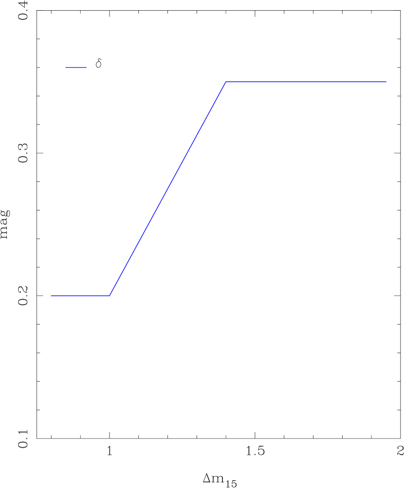
Figure 3: Width of the triangle function used, $\delta$, as a function of $\Delta$m₁₅. The values are chosen according to the sampling of the $\Delta$m${}_{15}(B)$ parameters of the templates in the template sample. Since we have only 4 templates with $\Delta{\rm m}_{15}>1.30$ mag, we use a wider triangle function for the fast declining templates.

In Figure 3 we show the value of $\delta$, the width of the triangle function as a function of $\Delta$m₁₅. The effect of this weighting scheme is that the discrete templates outside of the triangle function are given 0 weight. The larger values of $\delta$ for $\Delta$m${}_{15}>1.40$ mag were selected to overcome the poor sampling and small number of fast declining SNe in the template set (see Table A New Method to Calibrate the Magnitudes of Type Ia Supernovae at Maximum Light).

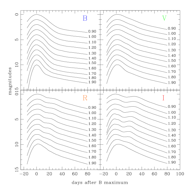
Figure 4: Constructed templates with a range of values of the $\Delta$m₁₅ parameter. These set of templates result from the interpolation of the discrete templates from the template set, using the triangle function. We have applied a progressive offset of 1 mag for plotting purposes.

In Figure 4 we present constructed templates with different values of $\Delta$m₁₅ as an example of the interpolation scheme. We have extrapolated the initial templates to earlier times ($-15\leq{\rm t-t}_{0}(B){\rm[days]}\leq-5$) assuming a quadratic dependence with time. The correlation between $\Delta$m₁₅, the post-maximum decline rate, and the rise time is very clear in the $BV$ templates: slow risers are slow decliners, and fast risers are fast decliners (Riess et al., 1999b). In the $RI$ templates this correlation is not clearly present, but it is observed that the secondary maximum occurs later for the slow declining LCs.

The final range of fitted $\Delta$m₁₅ values is restricted to the range in the input template set. For the template set presented in our work: $0.83\leq$ $\Delta$m${}_{15}{\rm\,[mag]}\leq 1.93$ (Table A New Method to Calibrate the Magnitudes of Type Ia Supernovae at Maximum Light).

3.2 $\chi^{2}$ fitting

In the original method (Phillips, 1993; Hamuy et al., 1996a, b; Phillips et al., 1999) and the modified version of Germany et al. (2004), $\Delta$m₁₅ is not fitted directly in one step. When a new LC is fitted, the total reduced $\chi^{2}$ is calculated for each template summed across all colors. The $\Delta$m₁₅ of the SN is derived with a second-order polynomial fit to the curve $\Delta$m₁₅ versus $\chi^{2}_{\nu}$, selecting the value where $\chi^{2}_{\nu}$ reaches a minimum as the best fitting parameter. This technique is justified by the fact that $\chi^{2}$ function changes quadratically with the parameters near the minimum (Bevington & Robinson, 1990; Press et al., 1988). This approach has two problems:

• the time of $B$ maximum, $BVRI$ magnitudes at maximum and $\Delta$m₁₅ are correlated parameters. This correlation is not considered in the quadratic fit to $\chi^{2}$.

• the statistical uncertainties in the best fitting value of $\Delta$m₁₅ are difficult to estimate in a consistent way.

The linear combination of templates weighted as described above, allows us to include $\Delta$m₁₅ directly in the $\chi^{2}$ function. In this way, the most general version of the empirical model for a new LC in the observed filter $Y$ is:

$$\vec{\mathcal{M}}^{Y}=\vec{\rm N}^{X}(\Delta{\rm m}_{15})+M_{max}^{X}(\Delta{\rm m}_{15})+\mu_{0}$$ (4)

$$+\vec{K}_{XY}(\Delta{\rm m}_{15},E(B-V))+\mathcal{R}_{X}\,E(B-V)_{host}+\mathcal{R}_{Y}\,E(B-V)_{Gal}$$

where: $M_{max}^{X}(\Delta{\rm m}_{15})$ are the relations between the absolute magnitude at maximum in the rest frame filter $X=BVRI$ and $\Delta{\rm m}_{15}$ (see Section 4 for the derivation of this relations); $\mu_{0}$ is the reddening corrected distance modulus of the SN; $\vec{K}_{XY}(\Delta{\rm m}_{15},E(B-V))$ are the cross-filter $K$-corrections (Kim, Goobar, & Perlmutter, 1996; Schmidt et al., 1998; Nugent, Kim, & Perlmutter, 2002; Germany et al., 2004), which depends on the colors of the SN and total extinction; $\mathcal{R}_{X}$ and $\mathcal{R}_{Y}$ are the ratio of total to selective extinction in the host galaxy and in the Milky Way, respectively; $E(B-V)_{host}$ and $E(B-V)_{Gal}$ are the color excesses in the host galaxy and in the Milky Way (Schlegel, Finkbeiner, & Davis, 1998).

When fitting a new SN LC we use this empirical model to construct a multidimensional $\chi^{2}$ function:

$$\chi^{2}({\rm t}_{0},\Delta{\rm m}_{15},E(B-V)_{host},\mu_{0})=[\vec{\mathcal{M}}^{Y}-\vec{m}^{Y}]^{T}({\bf C}^{Y})^{-1}[\vec{\mathcal{M}}^{Y}-\vec{m}^{Y}]$$ (5)

where $(\vec{\mathcal{M}}^{Y}-\vec{{m}}^{Y})$ are the residuals of the fit; $\vec{m}^{Y}$ are the observed magnitudes in the $Y$ filter (light curve data); ${\rm t}_{restframe}=({\rm t}_{obs}-{\rm t}_{0}(B))/(1+z)$, with $z$ the cosmological redshift, is the rest frame time which parametrizes the vectors; ${\bf C}^{Y}$ is the correlation matrix (Riess, Press, & Kirshner, 1996). This symmetric matrix contains the variances (squared statistical uncertainties) of the data for a given date (diagonal terms) and the correlation between data of different days in the same filter (non-diagonal terms). We use a diagonal matrix for ${\bf C}^{Y}$, setting the non-diagonal elements to zero, where each element takes into account the uncertainties in the data, the model, and the $K$-corrections: $\sigma_{data}^{2}+\sigma_{model}^{2}+\sigma_{K-corr}^{2}$. The uncertainties in the model, $\sigma_{model}$, are calculated by weighting the uncertainties in the observed templates with the same weights calculated from Equation 1.

The $\chi^{2}$ function of Equation 5 is minimized when a new SN light curve is fitted. This multidimensional (i.e. multicolor) minimization gives the best values for the parameters of the empirical model of Equation 4. The fitting parameters of the model are: time of $B$ maximum, $\Delta$m₁₅, color excess of the host galaxy, and the reddening corrected distance modulus.

Several works in the literature suggest that the average values of selective to total extinction of host galaxies are smaller than the Galactic values (Riess, Press, & Kirshner, 1996; Tripp & Branch, 1999; Phillips et al., 1999; Wang et al., 2003; Altavilla et al., 2004; Riendl et al., 2005). Also $\mathcal{R}$ changes in time because of the fast evolution of the SED of Type Ia SNe (Leibundgut, 1988; Phillips et al., 1999; Nugent, Kim, & Perlmutter, 2002; Jha, Riess, & Kirshner, 2006b), producing a dependence of $\Delta{\rm m}_{15}$ with the total extinction towards the SN. We have restricted in this work to constant values of $\mathcal{R}$, equal to the Galactic reddening law (Cardelli et al., 1989): $\mathcal{R}_{B}$=4.20, $\mathcal{R}_{V}$=3.10, $\mathcal{R}_{R}$=2.54, $\mathcal{R}_{I}$=1.85. In a future paper we will explore fitting the extinction law as part of the generalized $\chi^{2}$ fit.

To summarize, Equations 3 through 5 allow us to introduce a linear combination of templates directly into the $\chi^{2}$ fitting procedure. We do not have to output an intermediate table of interpolated templates (such as those shown in Figure 4). The mathematical framework allows us to change the weighting, the template set, and even the parameters to be fit in an elegant way.

3.3 Uncertainties in the fitting parameters

We calculate the uncertainties in the parameters of the best fitted LC model by constructing the covariance matrix. If we have $\chi^{2}(a_{i})$, with $a_{i}$ as the fitting parameters, the elements of the covariance matrix ${\bf\alpha}$ are (Bevington & Robinson, 1990; Press et al., 1988):

$$\alpha_{l,k}=\frac{1}{2}\frac{\partial^{2}\chi^{2}}{\partial a_{l}\partial a_{k}}$$ (6)

The partial derivatives are evaluated in the best fit parameters $a_{i}^{best}$. The inverse of the covariance matrix, the error matrix ${\bf\epsilon}={\bf\alpha^{-1}}$, has the variances (diagonal terms) and covariances (non-diagonal terms) in the best fitting parameters. The final $1\sigma$ uncertainties in the fitting parameters are estimated using the following approximate formula (Press et al., 1988):

$$\sigma_{a_{i}^{best}}=\sqrt{\chi^{2}_{\nu}\cdot\epsilon_{i,i}}$$ (7)

where: $\chi^{2}_{\nu}$ is the value of the minimum $\chi^{2}$ divided by the number of degree of freedom of the fit $\nu=N-m$, with $N$ the total number of data points fitted and $m$ the number of fitting parameters ($m=4$ in current implementation).

4 Calibration of the relations between $M_{max}$ and $\Delta{\rm m}_{15}$

The measurement of distances to Type Ia SNe using the $\Delta$m₁₅ method is based on the observed correlations between the absolutes magnitudes at maximum light ($M_{max}$) and the rate of evolution away from maximum light as parametrized originally with $\Delta$m₁₅ (Phillips, 1993; Hamuy et al., 1996a; Phillips et al., 1999; Germany et al., 2004) established with a low redshift sample of SNe in different rest frame filters (second term in the right hand side of Equation 4). Different versions of this relations have been proposed in the literature: linear relations (Phillips, 1993; Hamuy et al., 1996a), quadratic polynomials (Phillips et al., 1999; Germany et al., 2004), both restricted to $\Delta$m${}_{15}\leq 1.70$ mag, and an exponential that includes the fast declining light curves (Garnavich et al., 2004). Finally, a relation that includes both light curve shape and color (as a second parameter) has been published by Parodi et al. (2000).

We used a modified version of the analytical model of Equation 4 to fit the multicolor light curves of a large sample of Type Ia SNe at $z<0.12$ (see Table A New Method to Calibrate the Magnitudes of Type Ia Supernovae at Maximum Light) in order to study the relations between $M_{max}$ and $\Delta$m₁₅ in different filters. The parameters of this multicolor fits are: rest frame apparent $BVRI$ magnitudes at maximum corrected by Galactic and host reddening, $E(B-V)_{host}$, $\Delta$m₁₅, and time of maximum in $B$. This methodology is similar to the one applied by Germany et al. (2004) (section 4.4.4) in their modified $\Delta{\rm m}_{15}$ method. The main difference is that they used the unreddened sample of Type Ia SNe defined by Phillips et al. (1999), whereas we use a larger sample of SNe in a self consistent way analyzed with the analytical technique introduced in Section 3 to calculate $\Delta{\rm m}_{15}$ and $E(B-V)_{host}$ simultaneously from the multicolor light curves.

Since the magnitudes at maximum light and the host galaxy reddening are highly correlated parameters in the analytical model, priors are needed to soften this degeneracy. We applied them directly in the $\chi^{2}$ function as in Jha, Riess, & Kirshner (2006b). First, negative values of $E(B-V)_{host}$ were handled using a Bayesian filter (Riess, Press, & Kirshner, 1996), assuming a one sided Gaussian a priori distribution of $A_{B}$ with maximum at $A_{B}=0$ and $\sigma(A_{B})=0.3$ mag (Phillips et al., 1999). Secondly, Jha, Riess, & Kirshner (2006b) studied the intrinsic colors of a large sample of Type Ia SNe and found that their colors at 35 days after $B$ max are very homogeneous and well described by a Gaussian distribution with $(B-V)_{35}=1.055$ mag and $\sigma=0.055$ mag. We applied this as a prior in the reddening corrected $B-V$ colors, which is very similar to the “Lira law” (Lira, 1995). Because it is outside the scope of this paper, we leave as an open question how the host galaxy reddening obtained from the fits depends on the priors.

We assumed a concordance cosmology with $(h,\Omega_{M},\Omega_{\Lambda})=(0.72,0.3,0.7)$ to transform the rest frame apparent magnitudes to absolute magnitudes for SNe in the Hubble flow at redshifts $z>0.01$ (Calán/Tololo, CfAI, Krisciunas et al. and CfAII subsamples in Table A New Method to Calibrate the Magnitudes of Type Ia Supernovae at Maximum Light). For the nearby sample we used the distance moduli to the host galaxies obtained with the Surface Brightness Fluctuation method (Ajhar et al., 2001), matching the derived distances in $H_{0}=75[{\rm km\,s^{-1}\,Mpc^{-1}}]$ scale to $H_{0}=72[{\rm km\,s^{-1}\,Mpc^{-1}}]$. The final error budget in the absolute magnitudes includes: statistical uncertainties in the reddening corrected apparent magnitudes from the covariance matrix and a Hubble flow “noise” of 600 [km s^-1] to crudely model the effects of peculiar velocities (Marzke et al., 1995). For the nearby sample we only included the error in the distance modulus of the host galaxies.

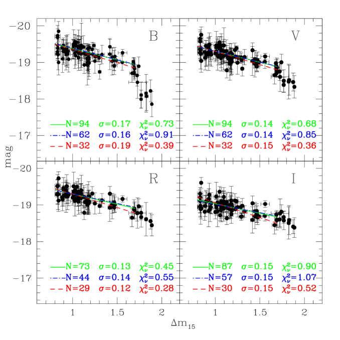
Figure 5: Relations between the absolute magnitudes at maximum and $\Delta{\rm m}_{15}$ in $BVRI$ filters. The lines are linear fits performed in the range $0.80<\Delta{\rm m}_{15}{\rm[mag]}<1.70$ to the complete sample (solid) of Table A New Method to Calibrate the Magnitudes of Type Ia Supernovae at Maximum Light, unreddened sample with $E(B-V)_{host}\leq 0.06$ mag (dot-dashed), and the reddened sample with $E(B-V)_{host}>0.06$ mag (dashed).

In Figure 5 we plot the results of the fits to the complete sample of Type Ia SNe listed Table A New Method to Calibrate the Magnitudes of Type Ia Supernovae at Maximum Light. For the SNe that are in common between Krisciunas et al. and CfAII sample (4 SNe), we have selected the results of the fits with smaller $\chi^{2}_{\nu}$ for the complete sample. The lines are linear fits to the relations between $\Delta m_{15}$ and $M_{max}$ in the range $0.80\leq\Delta m_{15}\leq 1.70$. We use $E(B-V)_{host}=0.06$ mag as a cut in host reddening for comparison with other works in the literature (e.g. Phillips et al. (1999)). In Table 3 we present the results of the various linear fits in different filters to the complete sample.

We restrict the linear fits to $\Delta m_{15}=1.70$ mag mainly because this cut has been widely used in other works of $\Delta m_{15}$ method (e.g. Phillips et al. (1999)). Garnavich et al. (2004) included subluminous (fast-declining) SNe to obtain distances, but the dispersion in the Hubble diagram increases and the sample of subluminous SNe is still small and poorly studied compared with normal SNe Ia.

We note that quadratic fits to the data, as the ones applied by Phillips et al. (1999), did not improve the reduced $\chi^{2}$ in this range of decline rates. Also, we did not take out SNe identified as outliers in previous papers because we cannot determine, in an unbiased way, if they are outliers in our analysis.

There are several important points to note about Figure 5. The dispersion around the linear fits does not correlate with wavelength, although the dispersion in $B$ is slightly bigger than in $VRI$ filters. This is probably due to a few SNe that deviate substantially from the whole sample, as it is evident in the Figure. This could be caused by a different reddening law in the host galaxies of this SNe, but varying the reddening law was outside the scope of the analysis presented here.

The zero-points of the linear relations are consistent, within the uncertainties, when we split the sample by host galaxy reddening. The slopes are marginally inconsistent, mainly in $R$ and $I$ filters, and steeper in the high-reddening sample. We think this is produced by the smaller number of fast declining SNe ($1.50<\Delta{\rm m}_{15}<1.70$) in the sample. The relations obtained here are consistent with previous works in the literature that include corrections for host galaxy reddening (Phillips et al., 1999; Germany et al., 2004).

In almost all the cases $\chi^{2}_{\nu}\lesssim 1.0$ in the linear fits, which could be produced by an overestimation of uncertainties in the absolute magnitudes. $\chi^{2}_{\nu}$ depends strongly in the adopted “noise” in the Hubble flow due to peculiar velocities which has values between 250-600 [km s^-1] in the literature (Baker, Davis & Lin, 2000; Landy, 2002; Zehavi et al., 2002; Hawkins et al., 2003). If we had chosen 400 [km s^-1] for instance, the values of $\chi^{2}_{\nu}$ would be $\sim 1.5$ times higher.

The dispersion around the linear fits seems to be larger at the lower end for the slowly declining SNe. This could be indication of a higher intrinsic dispersion in the slow decliners as noted by other authors. However, it is possible that the $\Delta{\rm m}_{15}$ values of some of these slow SNe are smaller than the minimum $\Delta{\rm m}_{15}$ of SNe in the template set. More well-sampled light curves of slow decliners are needed to extend and improve the template set in order to study the apparent larger natural dispersion.

In Table 4 we present the linear relations obtained for different subsamples in Table A New Method to Calibrate the Magnitudes of Type Ia Supernovae at Maximum Light. The zero-points of the linear relations are consistent, within the 1$\sigma$ uncertainties, in $RI$ filters. This is not the case in $BV$ filters where there is a clear difference (up to $\sim$0.17 mag in $B$) between CfAI, Krisciunas et. al and CfAII, which have consistent values, and Calán/Tololo which is brighter. The nearby sample is consistent with Calán/Tololo. This zero-point difference roughly represents the magnitude difference at $\Delta{\rm m}_{15}=1.1$ mag.

This same difference persists if we take the weighted average difference in the range $1.0\leq\Delta{\rm m}_{15}\leq 1.2$. This difference is $\sim 0.10\pm 0.03$ mag in $BV$ filters, with Calán/Tololo magnitudes again being brighter.

It is well known, but poorly studied, that photometry of SNe is sensitive to the throughput system of the telescope/filter/detector due the non-stellar nature of SN spectra (Suntzeff, 2000). Riess et al. (1999a) showed (their Table 1) that there are systematic differences in the observed photometry of SN1994D between the FLWO Observatory (CfAI and CfAII surveys) and CTIO data (Calán/Tololo survey). These differences are larger in the $B$ filter but always $<0.04$ mag, which are significantly less than the differences seen in absolute magnitudes at $\Delta{\rm m}_{15}=1.1$. However, the comparison of the absolute magnitudes in different data sets is not as simple because the absolute magnitudes at maximum are obtained from the fitting, which involves K-corrections and extinction corrections.

The systematic differences could arise from the poorly measured telescope/filter/detector transmission functions which define the natural photometric system. With accurate transmission functions and accurate atlases of spectrophotometry of SNe, we could calculate the S-corrections (Stritzinger et al., 2002) needed to bring the photometry of non-stellar SEDs onto a photometric standard system.

Another effect that could be introducing zeropoint shifts between subsamples is the existence of a Hubble bubble (Zehavi et al., 1998), a systematically lower expansion rate of $\sim 7\%$ measured for SNe Ia at $cz\geq 7400$ [km s^-1] (Jha, Riess, & Kirshner, 2006b). If we assume that the Hubble bubble alone is producing the systematic differences, the difference in zeropoints between Calán/Tololo and CfAI-II subsamples would be 0.06-0.09 mag. This effect does not fully explain the differences that we find.

The slopes of the linear fits in different subsamples, listed in Table 4, correct the SN peak magnitudes to a standard candle value. The slopes are consistent within the errors for Calán/Tololo, CfAI and Krisciunas et al. The shallower slopes of CfAII and nearby samples are produced by the SNe at high values of $\Delta\rm{m_{15}}$. Removing the SNe with $\Delta\rm{m_{15}}>1.5$ mag brings the slope of the CfAII sample into agreement with the fits to the other samples.

The dispersion around the linear fits are different between subsamples. For instance, the average dispersions in Calán/Tololo sample are smaller than the other subsamples (see Table 4. While the dispersion of Calán/Tololo for different filters is between $\sigma=0.11-0.14$ mag, CfAI and CfAII are in the range $\sigma=0.11-0.19$ and $\sigma=0.15-0.17$, respectively.

Part of the difference in dispersions could be due to the fact that the subsamples have different redshift coverage. We can compare the intrinsic dispersions subtracting off the effect of the random peculiar velocity of galaxies at the mean redshift of each subsample from the dispersions in Table 4, this is $\sigma_{int}^{2}=\sigma^{2}-\sigma_{v}^{2}$. The mean redshift of Calán/Tololo sample is $\bar{z}\simeq 0.05$ while for CfAI-II is $\bar{z}\simeq 0.02-0.03$. If we assume a random peculiar velocity of $\sigma_{v}$=400 [km s^-1] the intrinsic dispersions in the $B$ filter of Calán/Tololo, CfAI and CfAII are consistent within 0.03 mag, with $\sigma_{int}=0.09-0.12$ mag. This result is strongly dependent on the value of the peculiar velocity used.

The different dispersions and the different absolute magnitudes at $\Delta\rm{m_{15}}=1.1$ among the data subsamples point out the urgency in producing a new set of uniform SN light curves, taken preferably on a single telescope with a well calibrated telescope/filter/detector system. However, a more detailed analysis is needed to properly model the effects of a Hubble bubble in the zeropoints and the peculiar velocity field of galaxies, coupled with the real redshift distributions of subsamples, this could explain in part the differences observed.

5 Hubble diagram of low-$z$ Type Ia SNe

With the relations for $M_{max}(\Delta\rm{m_{15}})$ in different filters (RHS of Equation 4), we can now apply our fitting technique minimizing the $\chi^{2}$ function in Equation 5 to obtain the distance modulus of a large sample of SNe in the Hubble flow. We use the complete sample of 89 SNe in Table A New Method to Calibrate the Magnitudes of Type Ia Supernovae at Maximum Light with $z>0.01$ and $\Delta\rm{m_{15}}\leq 1.70$ mag. The results of the fits are presented in Table 5 where we give the best fit parameters ($\Delta{\rm m_{15}},\,E(B-V)_{host},\,\mu_{0}$) including their statistical errors from the covariance matrix. We plot all the light curves and best fit models in Figures 7-16. We obtained a median value of $\chi^{2}_{\nu}=1.3$ for all the fits.

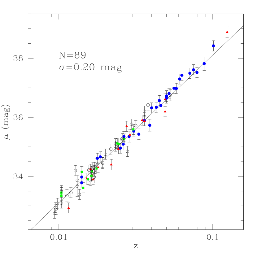
Figure 6: Hubble Diagram of the complete sample of SNe with $z>0.01$ and $\Delta m_{15}\leq 1.70$ mag (89). The symbols correspond to different subsamples of SNe: Calán/Tololo (filled circles), CfAI (filled triangles), Krisciunas et al. (filled squares), and CfAII (open circles).

In Figure 6 we plot the Hubble diagram constructed with results of the fits to the 89 SNe in the Hubble flow. The final error in the distance modulus is obtained by adding in quadrature the statistical uncertainties from the covariance matrix and 0.17 mag, which is the maximum natural dispersion in the relations $M_{max}(\Delta\rm{m_{15}})$ obtained in Section 4. At these low redshifts, we can ignore the cosmological effects and fit the Hubble law as the second order expansion of the luminosity distance with $\Omega_{M}=0$ and $\Omega_{\Lambda}=0$: $d_{L}(z)\simeq(cz/H_{0})(1+z/2)$. We find that the dispersion in the Hubble diagram is $\sigma=0.20$ mag using 89 SNe. This is a $9\%$ error in distance to a single SN, a very accurate distance estimator considering the large sample of SNe studied. As a comparison, Jha, Riess, & Kirshner (2006b) obtains $\sigma=0.18$ mag using 95 SNe in the same redshift range.

In Table 6, we compare the dispersion in the Hubble diagram with other results in the literature, using the same SNe as in the original papers. In general we find similar or smaller values for the dispersion, with the Calán/Tololo subsample giving the fit with the lowest dispersion. The dispersion varies in the range $\sigma=0.14-0.21$ mag with our technique and between $\sigma=0.14-0.24$ mag for results in the literature, using identical samples of SNe. This further demonstrates that our technique performs equally well or better than other existing techniques in the literature. To reduce the dispersion in the Hubble diagram further will require new uniform data sets, realistic priors that allow different reddening laws for the host galaxies, and careful attention to the calibration of the telescope/filter/detector system required by the S-corrections.

6 Conclusions

We have presented an empirical method to fit multicolor light curves of Type Ia supernovae and estimate their luminosity distances. This technique combines what we think are the advantages from two widely used methods in the literature: the $\Delta$m₁₅ template fitting method (Phillips et al., 1999), and MLCS (Riess, Press, & Kirshner, 1996).

Our basic fitting algorithm uses a set of 14 $BVRI$ light curve templates with different values of $\Delta$m${}_{15}(B)$ and a simple triangle weighting function. A linear combination of the templates, weighted by this function, is introduced directly into the $\chi^{2}$ fitting, avoiding the construction of a secondary grid of interpolated templates. This allows us to add or change templates trivially, and also allows us to introduce other parameters to be fit in the $\chi^{2}$ minimization. The $\chi^{2}$ fit returns the $1\sigma$ uncertainties in the best fit parameters from the covariance matrix.

From a sample of 94 nearby Type Ia SNe ($z\lesssim 0.1$) we established linear relations between the absolute magnitudes at maximum $M_{max}$ and $\Delta$m₁₅ in $BVRI$ filters. These relations are valid in the range $0.80<\Delta{\rm m}_{15}{\rm[mag]}<1.70$ and they are consistent with other results presented in the literature (Phillips et al., 1999; Garnavich et al., 2004; Germany et al., 2004). We studied the relations using different subsamples of SNe, associated with different surveys and publications in the literature: Calán/Tololo, CfAI, Krisciunas et al., CfAII and a nearby sample ($z\lesssim 0.01$) with distances obtained from SBF method. The results from different subsamples are consistent in almost all the cases when we compare the slopes and zero-points of the linear relations in the same filter, but disturbing differences do exist mainly in $B$ and $V$ absolute magnitudes at $\Delta m_{15}=1.1$. Further progress will require new light curve data sets, realistic priors that allow different reddening laws, and careful attention to the calibration of the telescope/filter/detector system required by the S-corrections.

We have constructed a Hubble diagram with low-$z$ SNe fitting the light curves of 89 SNe in the Hubble flow. The dispersion of the Hubble diagram is $\sigma=0.20$ mag or an error of $\sim 9\%$ in distance to single objects, consistent with other fitting techniques (Jha, Riess, & Kirshner, 2006b; Germany et al., 2004). We compared the dispersion in the Hubble diagram using our technique with other results in the literature. In general our technique give similar or smaller dispersions than published results when the comparison is made using identical samples of SNe.

Table 1: Basic information of the light curve templates in the template set.

SN	$\Delta$m15	$E(B-V)_{Gal}$	$\Delta$mV	$\Delta$mR	$\Delta$mI	Ref
(1)	(2)	(3)	(4)	(5)	(6)	(7)
1991T	0.94	0.022	-0.02	-0.01	0.00	1, 2
1991bg	1.93	0.040	-0.05	-0.14	-0.10	1, 5, 6
1992A	1.47	0.017	-0.03	-0.03	-0.05	1, 4
1992al	1.11	0.034	0.00	-0.02	-0.01	1, 3
1992bc	0.87	0.022	0.00	0.00	-0.02	1, 3
1992bo	1.69	0.027	0.00	0.00	-0.02	1, 3
1994D	1.34	0.022	0.00	0.00	-0.10	7
1994ae	0.94	0.031	-0.01	0.00	0.00	8
1995D	1.05	0.058	0.00	0.00	0.00	8
1995al	0.89	0.014	-0.01	-0.01	-0.01	8
1996X	1.25	0.069	-0.02	0.00	-0.07	9
1998bu	1.05	0.025	0.00	-0.01	-0.05	10, 11
1999aa	0.83	0.015	-0.02	-0.02	-0.03	12, 13
2001el	1.12	0.014	-0.03	-0.01	-0.06	14

Note. — The columns are: (1) name of the supernova; (2) $\Delta$m${}_{15}(B)$ from the $B$ light curve template; (3) $V_{max}-V_{t_{0}}$; (4) $R_{max}-R_{t_{0}}$; (5) $I_{max}-I_{t_{0}}$; (6) References containing the data with the light curves used to construct the templates.

References. — (1) Hamuy et al. 1996d; (2) Lira et al. 1998; (3) Hamuy et al. 1996c; (4) Suntzeff et al. (unpublished); (5) Filippenko et al. 1992; (6) Leibundgut et al. 1993; (7) Smith et al. (unpublished); (8) Riess et al. 1999a; (9) Covarrubias et al. (unpublished); (10) Jha et al. 1999; (11) Suntzeff et al. 1999; (12) Krisciunas et al. 2000; (13) Jha et al. 2006a; (14) Krisciunas et al. 2003

Table 2: Different samples of SNe used to study the relations between absolutes magnitudes at maximum ($M_{max}$) and $\Delta{\rm m}_{15}$.

Sample	SN	Ref
Calán/Tololo	90O, 90T, 90Y, 90af, 91S, 91U, 91ag, 92ae, 92al,	1
	92bc, 92J, 92P, 92ag, 92aq, 92au, 92bg, 92bh,
	92bk, 92bl, 92bo, 92bp, 92br, 92bs, 93B, 93O,
	93ag, 93ah
CfAI	93ac, 93ae, 94M, 94Q, 94S, 94T, 95E, 95ac, 95ak,	2
	95bd, 96C, 96ab, 96bl, 96bo, 96bv
Krisciunas et al.	99aa, 99cp, 99dk, 99ee, 99ek, 99gp, 00bh, 00bk,	3, 4, 5, 6, 7
	00ca, 00ce, 01ba, 01bt, 01cn, 01cz
CfAII	97E, 97Y, 97cw, 97dg, 97do, 98D, 98V, 98ab, 98co,	8
	98dk, 98dx, 98ec, 98ef, 98eg, 99X, 99aa, 99ac,
	99cc, 99cw, 99dq, 99ef, 99ej, 99ek, 99gd, 99gp,
	00B, 00ce, 00cf, 00cn, 00dk, 00fa
Nearby	72E, 80N, 81B, 86G, 89B, 90N, 91T, 92A, 94D, 95D,	1, 2, 7, 8, 11, 12, 13, 14, 15, 16,
	96X, 96bk, 98aq, 98bu, 99by, 02bo	17, 18, 19, 20, 21, 22, 23, 24, 25

Note. — The columns are: (1) Name of the data sample; (2) Supernova in the sample; (3) References.

References. — (1) Hamuy et al. 1996c; (2) Riess et al. 1999a; (3) Krisciunas et al. 2000; (4) Krisciunas et al. 2001; (5) Stritzinger et al. 2002; (6) Krisciunas et al. 2004b; (7) Krisciunas et al. 2004c; (8) Jha et al. 2006a; (9) Ardeberg & de Groot 1973; (10) van Genderen 1975; (11) Lee et al. 1972; (12) Cousins 1972; (13) Hamuy et al. 1991; (14) Barbon, Ciatti & Rosino 1982; (15) Buta & Turner 1983; (16) Phillips et al. 1987; (17) Cristiani et al. 1992; (18) Schaefer 1987; (19) Barbon et al. 1990; (20) Wells et al. 1994; (21) Lira et al. 1998; (22) Smith et al. (unpublished); (23) Covarrubias et al. (unpublished); (24) Boffi et al. (unpublished); (25) Garnavich et al. 2004.

Table 3: Best fit linear relations to $M_{max}$ versus $\Delta m_{15}$ in $BVRI$ filters for the complete sample (ALL). The assumed linear relations are of the form: $M_{max}=a+b(\Delta m_{15}-1.1)$ in the range $0.80\leq\Delta m_{15}\leq 1.70$. We also give the linear fits using a cut in host galaxy color excess at $E(B-V)_{host}=0.06$ mag.

Filter	$a$	$b$	$\sigma$	$\chi^{2}_{\nu}$	N
ALL
$B$	$-$19.319(022)	0.634(077)	0.17	0.73	94
$V$	$-$19.246(019)	0.606(069)	0.14	0.68	94
$R$	$-$19.248(025)	0.566(101)	0.13	0.45	73
$I$	$-$18.981(020)	0.524(079)	0.15	0.90	87
$E(B-V)_{host}\leq 0.06$ mag
$B$	$-$19.325(024)	0.636(082)	0.16	0.91	62
$V$	$-$19.247(022)	0.598(075)	0.14	0.85	62
$R$	$-$19.251(031)	0.522(012)	0.14	0.55	44
$I$	$-$18.975(023)	0.464(090)	0.15	1.07	57
$E(B-V)_{host}>0.06$ mag
$B$	$-$19.286(051)	0.753(255)	0.19	0.39	32
$V$	$-$19.233(044)	0.748(226)	0.15	0.36	32
$R$	$-$19.229(044)	0.761(216)	0.12	0.28	29
$I$	$-$18.983(038)	0.825(196)	0.15	0.52	30

Note. — The columns are: (1) filter; (2) zero-point of the linear fits with uncertainties in parentheses, in units of 0.001 mag; (3) slope of the linear fits with uncertainties in parentheses, in units of 0.001 mag; (4) rms scatter of each sample around the linear fits; (5) $\chi^{2}$ per degree of freedom of the fits; (6) number of SNe.

Table 4: Best fit linear relations $M_{max}$ versus $\Delta m_{15}$ in $BVRI$ filters for different sub-samples of Table A New Method to Calibrate the Magnitudes of Type Ia Supernovae at Maximum Light.

Filter	$a$	$b$	$\sigma$	$\chi^{2}_{\nu}$	N
Cálan/Tololo
$B$	$-$19.376(037)	0.814(118)	0.11	0.80	27
$V$	$-$19.295(032)	0.773(105)	0.11	0.97	27
$R$	$-$19.249(062)	1.003(364)	0.13	0.56	9
$I$	$-$18.974(032)	0.559(130)	0.14	1.49	23
CfAI
$B$	$-$19.224(055)	0.880(210)	0.19	0.56	15
$V$	$-$19.167(049)	0.659(187)	0.16	0.61	15
$R$	$-$19.269(059)	0.721(205)	0.11	0.33	14
$I$	$-$19.049(053)	0.787(193)	0.16	0.98	14
Krisciunas et al.
$B$	$-$19.279(084)	1.224(570)	0.21	0.51	13
$V$	$-$19.218(082)	1.159(551)	0.16	0.32	13
$R$	$-$19.192(091)	0.868(546)	0.12	0.21	12
$I$	$-$18.958(078)	0.406(520)	0.12	0.21	13
CfAII
$B$	$-$19.209(049)	0.246(153)	0.15	0.46	30
$V$	$-$19.171(046)	0.307(145)	0.14	0.40	30
$R$	$-$19.188(044)	0.349(142)	0.14	0.47	30
$I$	$-$18.941(042)	0.283(141)	0.17	0.77	30
Nearby
$B$	$-$19.343(051)	0.166(284)	0.14	0.42	16
$V$	$-$19.265(046)	0.398(262)	0.12	0.34	16
$R$	$-$19.259(046)	0.515(263)	0.12	0.37	15
$I$	$-$18.986(044)	0.478(242)	0.13	0.47	14

Note. — The columns are: (1) filter; (2) zeropoint of the linear fits with uncertainties in parentheses, in units of 0.001 mag; (3) slope of the linear fits with uncertainties in parentheses, in units of 0.001 mag; (4) rms scatter of each subsample/filter around the linear fits; (5) $\chi^{2}$ per degree of freedom of the linear fits; (6) number of SNe.

Table 5: Final results of the $\Delta$m₁₅ fits to the light curves of 89 Type Ia SNe in the Hubble flow ($0.01<z<0.10$).

SN	$z$	$\mu_{0}(\sigma)$	$E(B-V)_{host}(\sigma)$	$\Delta$m${}_{15}(\sigma)$
(1)	(2)	(3)	(4)	(5)
1990O	0.0307	35.535(0.028)	0.003(0.008)	1.019(0.017)
1990T	0.0401	36.321(0.026)	0.017(0.010)	1.120(0.017)
1990Y	0.0390	35.733(0.112)	0.194(0.023)	1.273(0.030)
1990af	0.0500	36.648(0.017)	0.006(0.006)	1.681(0.010)
1991S	0.0560	36.987(0.023)	0.001(0.005)	1.036(0.021)
1991U	0.0331	35.431(0.049)	0.092(0.022)	0.929(0.018)
1991ag	0.0141	33.782(0.027)	0.000(0.004)	0.975(0.023)
1992J	0.0460	36.400(0.079)	0.031(0.030)	1.662(0.045)
1992P	0.0265	35.350(0.021)	0.006(0.006)	1.088(0.019)
1992ae	0.0750	37.610(0.041)	0.007(0.011)	1.212(0.025)
1992ag	0.0262	35.092(0.103)	0.106(0.027)	1.162(0.026)
1992al	0.0141	33.978(0.040)	0.000(0.005)	0.916(0.050)
1992aq	0.1010	38.421(0.042)	0.000(0.009)	1.273(0.022)
1992au	0.0610	37.297(0.040)	0.005(0.011)	1.259(0.021)
1992bc	0.0186	34.663(0.032)	0.000(0.007)	0.838(0.030)
1992bg	0.0360	35.893(0.057)	0.002(0.011)	1.179(0.020)
1992bh	0.0450	36.567(0.033)	0.085(0.011)	1.065(0.018)
1992bk	0.0580	36.977(0.040)	0.018(0.015)	1.677(0.010)
1992bl	0.0430	36.340(0.025)	0.000(0.005)	1.515(0.030)
1992bo	0.0178	34.614(0.014)	0.015(0.006)	1.688(0.001)
1992bp	0.0790	37.518(0.024)	0.000(0.006)	1.238(0.018)
1992br	0.0880	37.819(0.158)	0.075(0.053)	1.690(0.010)
1992bs	0.0630	37.426(0.072)	0.033(0.025)	1.076(0.017)
1993B	0.0710	37.495(0.052)	0.037(0.019)	1.097(0.014)
1993H	0.0251	34.957(0.034)	0.153(0.012)	1.700(0.010)
1993O	0.0520	36.801(0.036)	0.016(0.013)	1.207(0.012)
1993ac	0.0490	36.608(0.077)	0.134(0.032)	1.068(0.021)
1993ae	0.0180	34.308(0.026)	0.000(0.004)	1.560(0.025)
1993ag	0.0500	36.724(0.063)	0.064(0.015)	1.225(0.017)
1993ah	0.0286	35.346(0.067)	0.028(0.030)	1.285(0.017)
1994M	0.0244	34.930(0.029)	0.113(0.011)	1.376(0.022)
1994Q	0.0290	35.405(0.041)	0.037(0.018)	1.064(0.012)
1994S	0.0161	34.247(0.014)	0.000(0.006)	0.859(0.010)
1994T	0.0360	35.877(0.036)	0.111(0.013)	1.475(0.010)
1995E	0.0116	32.929(0.045)	0.720(0.013)	1.170(0.019)
1995E	0.0116	33.141(0.055)	0.721(0.020)	0.830(0.030)
1995ac	0.0490	36.193(0.035)	0.090(0.012)	0.830(0.010)
1995ak	0.0219	34.398(0.066)	0.208(0.021)	1.303(0.017)
1995bd	0.0152	33.927(0.081)	0.140(0.032)	0.909(0.035)
1996C	0.0276	35.695(0.030)	0.041(0.009)	1.011(0.013)
1996ab	0.1240	38.884(0.036)	0.000(0.009)	1.064(0.015)
1996bl	0.0348	35.903(0.038)	0.061(0.015)	0.830(0.030)
1996bo	0.0165	34.028(0.072)	0.305(0.028)	0.830(0.010)
1996bv	0.0167	33.897(0.036)	0.190(0.014)	0.940(0.019)
1997E	0.0132	33.871(0.032)	0.054(0.012)	1.514(0.024)
1997Y	0.0166	34.302(0.053)	0.065(0.015)	1.132(0.026)
1997bp	0.0094	32.756(0.052)	0.132(0.017)	0.830(0.010)
1997bq	0.0095	32.944(0.018)	0.086(0.006)	1.467(0.010)
1997cn	0.0175	34.437(0.061)	0.192(0.023)	1.686(0.010)
1997cw	0.0160	33.863(0.060)	0.322(0.009)	0.906(0.060)
1997dg	0.0297	35.768(0.053)	0.085(0.015)	1.203(0.024)
1997do	0.0104	33.508(0.064)	0.081(0.022)	0.830(0.020)
1998D	0.0132	33.672(0.305)	0.186(0.060)	1.697(0.010)
1998V	0.0170	34.187(0.075)	0.064(0.023)	0.983(0.040)
1998ab	0.0279	34.851(0.043)	0.212(0.013)	0.832(0.010)
1998bp	0.0104	33.097(0.053)	0.251(0.020)	1.700(0.010)
1998co	0.0171	34.288(0.084)	0.172(0.031)	0.845(0.014)
1998dk	0.0120	33.453(0.051)	0.140(0.017)	1.140(0.022)
1998dx	0.0530	36.753(0.096)	0.050(0.032)	1.063(0.028)
1998ec	0.0201	34.752(0.048)	0.161(0.022)	1.074(0.014)
1998ef	0.0170	33.979(0.112)	0.132(0.036)	0.830(0.010)
1998eg	0.0234	35.102(0.060)	0.085(0.021)	1.062(0.035)
1998es	0.0096	32.885(0.016)	0.076(0.006)	0.917(0.007)
1999X	0.0257	35.256(0.062)	0.079(0.029)	0.958(0.027)
1999aa	0.0157	34.215(0.023)	0.000(0.007)	0.837(0.020)
1999ac	0.0098	33.090(0.026)	0.081(0.009)	1.067(0.010)
1999cc	0.0316	35.718(0.037)	0.035(0.012)	1.408(0.026)
1999cp	0.0104	33.452(0.034)	0.002(0.007)	0.838(0.030)
1999cw	0.0113	33.349(0.124)	0.010(0.042)	0.830(0.020)
1999dk	0.0141	34.157(0.056)	0.000(0.020)	0.830(0.010)
1999dq	0.0136	33.390(0.016)	0.092(0.006)	0.941(0.010)
1999ee	0.0104	33.349(0.015)	0.230(0.005)	0.830(0.010)
1999ef	0.0380	36.417(0.044)	0.000(0.010)	1.065(0.015)
1999ej	0.0128	34.197(0.043)	0.051(0.017)	1.534(0.029)
1999ek	0.0176	34.268(0.070)	0.157(0.027)	1.058(0.034)
1999gd	0.0193	34.451(0.074)	0.411(0.022)	1.180(0.025)
1999gp	0.0260	35.280(0.032)	0.034(0.010)	0.832(0.010)
2000B	0.0193	34.470(0.038)	0.075(0.015)	1.300(0.016)
2000bh	0.0240	35.118(0.021)	0.001(0.003)	1.129(0.009)
2000bk	0.0266	35.267(0.048)	0.146(0.020)	1.700(0.010)
2000ca	0.0245	35.092(0.017)	0.000(0.005)	0.858(0.010)
2000ce	0.0164	34.170(0.037)	0.513(0.016)	0.998(0.031)
2000cf	0.0360	36.207(0.031)	0.023(0.013)	1.157(0.019)
2000cn	0.0233	35.023(0.036)	0.099(0.013)	1.700(0.010)
2000dk	0.0164	34.246(0.013)	0.004(0.006)	1.690(0.010)
2000fa	0.0218	34.925(0.029)	0.063(0.011)	1.049(0.016)
2001ba	0.0305	35.590(0.013)	0.000(0.004)	1.054(0.010)
2001bt	0.0144	33.616(0.036)	0.214(0.011)	1.170(0.014)
2001cn	0.0155	33.901(0.019)	0.128(0.006)	1.152(0.010)
2001cz	0.0163	34.025(0.032)	0.096(0.009)	0.977(0.018)

Note. — The columns are: (1) name of the supernova; (2) redshift in the CMB frame; (3) best fit distance modulus ($h=0.72$), statistical errors in parentheses; (4) best fit color excess $E(B-V)_{host}$, statistical errors in parentheses; (5) best fit $\Delta{\rm m}_{15}$, statistical errors in parentheses.

Table 6: Comparison of rms dispersion in the Hubble diagram using the technique presented in this paper with other results in the literature.

Literature	$\sigma_{\rm Literature}$	$\sigma_{\rm This\,Work}$	Number of SNe
Phillips et al. (1999)	0.14	0.14	26
Knop et al. (2003)	0.20	0.16	23
Riess et al. (2004)	0.24	0.19	68
Germany et al. (2004)	0.23	0.19	42
Reindl et al. (2005)	0.21	0.21	71

Figure 2: Weighting function used for the interpolation between the observed discrete templates in the template set. The value of the weight assigned to each template, $w_{i}$, is equal to the value of the triangle function in the $\Delta$m${}_{15}(B)$ of the template $i$. The weights are normalized so that they sum to 1. When a new light curve fitting is performed, the center of the triangle function, $\Delta{\rm m}_{0}$, moves freely in the $\Delta$m₁₅ axis until the $\chi^{2}$ of the fit is minimized. The final value of the $\Delta$m₁₅ of the constructed template is obtained by weighting the values of the template set.

Figure 7: Results of the fits to the multicolor light curves. The different filters (symbols) are: $B$ (squares), $V$ (triangles), $R$ (circles) and $I$ (rhombuses). To avoid overlap between different filters we applied shifts to the relative magnitudes: $\Delta B$, $\Delta V$-1, $\Delta R$-2, $\Delta I$-3.

Figure 8: Results of the fits to the multicolor light curves. The different filters (symbols) are: $B$ (squares), $V$ (triangles), $R$ (circles) and $I$ (rhombuses). To avoid overlap between different filters we applied shifts to the relative magnitudes: $\Delta B$, $\Delta V$-1, $\Delta R$-2, $\Delta I$-3.

Figure 9: Results of the fits to the multicolor light curves. The different filters (symbols) are: $B$ (squares), $V$ (triangles), $R$ (circles) and $I$ (rhombuses). To avoid overlap between different filters we applied shifts to the relative magnitudes: $\Delta B$, $\Delta V$-1, $\Delta R$-2, $\Delta I$-3.

Figure 10: Results of the fits to the multicolor light curves. The different filters (symbols) are: $B$ (squares), $V$ (triangles), $R$ (circles) and $I$ (rhombuses). To avoid overlap between different filters we applied shifts to the relative magnitudes: $\Delta B$, $\Delta V$-1, $\Delta R$-2, $\Delta I$-3.

Figure 11: Results of the fits to the multicolor light curves. The different filters (symbols) are: $B$ (squares), $V$ (triangles), $R$ (circles) and $I$ (rhombuses). To avoid overlap between different filters we applied shifts to the relative magnitudes: $\Delta B$, $\Delta V$-1, $\Delta R$-2, $\Delta I$-3.

Figure 12: Results of the fits to the multicolor light curves. The different filters (symbols) are: $B$ (squares), $V$ (triangles), $R$ (circles) and $I$ (rhombuses). To avoid overlap between different filters we applied shifts to the relative magnitudes: $\Delta B$, $\Delta V$-1, $\Delta R$-2, $\Delta I$-3.

Figure 13: Results of the fits to the multicolor light curves. The different filters (symbols) are: $B$ (squares), $V$ (triangles), $R$ (circles) and $I$ (rhombuses). To avoid overlap between different filters we applied shifts to the relative magnitudes: $\Delta B$, $\Delta V$-1, $\Delta R$-2, $\Delta I$-3.

Figure 14: Results of the fits to the multicolor light curves. The different filters (symbols) are: $B$ (squares), $V$ (triangles), $R$ (circles) and $I$ (rhombuses). To avoid overlap between different filters we applied shifts to the relative magnitudes: $\Delta B$, $\Delta V$-1, $\Delta R$-2, $\Delta I$-3.

Figure 15: Results of the fits to the multicolor light curves. The different filters (symbols) are: $B$ (squares), $V$ (triangles), $R$ (circles) and $I$ (rhombuses). To avoid overlap between different filters we applied shifts to the relative magnitudes: $\Delta B$, $\Delta V$-1, $\Delta R$-2, $\Delta I$-3.

Figure 16: Results of the fits to the multicolor light curves. The different filters (symbols) are: $B$ (squares), $V$ (triangles), $R$ (circles) and $I$ (rhombuses). To avoid overlap between different filters we applied shifts to the relative magnitudes: $\Delta B$, $\Delta V$-1, $\Delta R$-2, $\Delta I$-3.

References

- (1)
- Ajhar et al. (2001) Ajhar, E. A., Tonry, J. T., Blakeslee, J. P., Riess, A. G., & Schmidt, B. P. 2001, ApJ, 559, 584
- Altavilla et al. (2004) Altavilla, G., Fiorentino, G., Marconi, M., et al. 2004, MNRAS, 349, 1344
- Ardeberg & de Groot (1973) Ardeberg, A., & de Groot, M. 1973, A&A, 28, 295
- Arnett (1982) Arnett, W. D. 1982, ApJ, 253, 785
- Baker, Davis & Lin (2000) Baker, J. E., Davis, M., & Lin, H. 2000, ApJ, 536, 112
- Barbon, Ciatti & Rosino (1982) Barbon, R., Ciatti, F., & Rosino, L. 1982, A&A, 116, 35
- Barbon et al. (1990) Barbon, R., Bennetti, S., Rosino, L., et al. 1990, A&A, 237, 79
- Bevington & Robinson (1990) Bevington, P. R., & Robinson, D. K. 1992, Data Reduction and Error Analysis for the Physical Sciences, McGraw-Hill, Inc.
- Branch (1987) Branch, D. 1987, ApJ, 316, L81
- Buta & Turner (1983) Buta, R. J., & Turner, A. 1983, PASP, 95, 72
- Cardelli et al. (1989) Cardelli, J. A., Clayton, G. C., & Mathis, J. S. 1989, ApJ, 345, 245
- Carroll, Press, & Turner (1992) Carroll, S. M., Press, W. H., & Turner, E. L. 1992, ARA&A, 30, 499
- Cousins (1972) Cousins, A, W., J. 1972, BVS, 700, 1
- Cristiani et al. (1992) Cristiani, S., Capellaro, E., Turatto, M., et al. 1992, A&A, 259, 63
- Filippenko et al. (1992) Filippenko, A. V., Richmond, M. W., Branch, D., et al. 1992, AJ, 104, 1543
- Garnavich et al. (2004) Garnavich, P. M., Bonanos, A. Z., Krisciunas, K., et al. 2004, ApJ, 613, 1120
- Germany et al. (2004) Germany, L. M., Reiss, D. J., Schmidt, B. P., Stubbs, C. W., & Suntzeff, N. B. 2004, A&A, 415, 863
- Goldhaber et al. (2001) Goldhaber, G., Groom, D. E., Kim, A., et al. 2001, ApJ, 558, 359
- Hawkins et al. (2003) Hawkins, E., Maddox, S., Cole, S., et al. 2003, MNRAS, 346, 78
- Hamuy et al. (1991) Hamuy, M., Phillips, M. M., Maza, J., et al. 1991, AJ, 102, 208
- Hamuy et al. (1993) Hamuy, M., Phillips, M. M., Wells, L. A., & Maza, J. 1993, PASP, 105, 787
- Hamuy et al. (1996a) Hamuy, M., Phillips, M. M., Suntzeff, N. B., Schommer, R. A., Maza, J., & Aviles, R. 1996a, AJ, 112, 2391
- Hamuy et al. (1996b) Hamuy, M., Phillips, M. M., Suntzeff, N. B., Schommer, R. A., Maza, J., & Aviles, R. 1996b, AJ, 112, 2398
- Hamuy et al. (1996c) Hamuy, M., Phillips, M. M., Suntzeff, N. B., et al. 1996c, AJ, 112, 2408
- Hamuy et al. (1996d) Hamuy, M., Phillips, M. M., Suntzeff, N. B., Schommer, R. A., Maza, J., Smith, R. C., Lira, P., & Aviles, R. 1996d, AJ, 112, 2438
- Jha et al. (2006a) Jha, S., Kirshner, R. P., Challis, P., et al. 2006, AJ, accepted
- Jha, Riess, & Kirshner (2006b) Jha, S., Riess, A. G., & Kirshner, R. P. 2006, ApJ, submitted
- Jha et al. (1999) Jha, S., Garnavich, P. M., Kirshner, R. P., et al. 1999, ApJS, 125, 73
- Kim, Goobar, & Perlmutter (1996) Kim, A., Goobar, A., & Perlmutter, S. 1996, PASP, 108, 190
- Krisciunas et al. (2000) Krisciunas, K., Hastings, N. C., Loomis, K., et al. 2000, ApJ, 539, 658
- Krisciunas et al. (2001) Krisciunas, K., Phillips, M. M., Stubbs, C., et al. 2001, AJ, 122, 1616
- Krisciunas et al. (2003) Krisciunas, K., Suntzeff, N. B., Candia, P., et al. 2003, AJ, 125, 166
- Krisciunas et al. (2004b) Krisciunas, K., Phillips, M. M., Suntzeff, N. B., et al. 2004b, AJ, 127, 1664
- Krisciunas et al. (2004c) Krisciunas, K., Suntzeff, N. B., Phillips, M. M., et al. 2004c, AJ, 128, 303
- Landy (2002) Landy, S. D. 2002, ApJ, 567, L1
- Lee et al. (1972) Lee, T. A., Wamsteker, W., Wisniewski, W. Z., & Wdowiak, T. J. 1972, ApJ, 177, L59
- Leibundgut (1988) Leibundgut, B. 1988, Ph.D. Thesis, University of Basel
- Leibundgut et al. (1993) Leibundgut, B., Kirshner, R. P., Phillips, M. M. 1993, AJ, 105, 301
- Leibundgut (2000) Leibundgut, B. 2000, A&A Rev., 10, 179
- Lira (1995) Lira, P. 1995, Masters thesis, Universidad de Chile
- Lira et al. (1998) Lira, P., Hamuy, M., Wells, L. A., et al. 1998, AJ, 115, 234
- Marzke et al. (1995) Marzke, R. O., Geller, M. J., da Costa, L. N., & Huchra, J. P. 1995, AJ, 110, 447
- Nugent, Kim, & Perlmutter (2002) Nugent, P., Kim, A., & Perlmutter, S. 2002, PASP, 114, 803
- Parodi et al. (2000) Parodi, B. R., Saha, A., Sandage, A., & Tammann, G. A. 2000, ApJ, 540, 634
- Perlmutter et al. (1997) Perlmutter, S., Gabi, S., Goldhaber, G., et al. 1997, ApJ, 483, 565
- Perlmutter et al. (1999) Perlmutter, S., Aldering, G., Goldhaber, et al. 1999, ApJ, 517, 565
- Phillips et al. (1987) Phillips, M. M., Phillips, A. C., Heathcote, S. R., et al. 1987, PASP, 99, 592
- Phillips (1993) Phillips, M. M. 1993, ApJ, 413, L105
- Phillips et al. (1999) Phillips, M. M., Lira, P., Suntzeff, N. B., Schommer, R. A., Hamuy, M., & Maza, J. 1999, AJ, 118, 1766
- Press et al. (1988) Press, W. H., Teukolsky, S. A., Vetterling, W. T., & Flannery, B. P. 1988, Numerical Recipes in C, Cambridge University Press.
- Pskovskii (1977) Pskovskii, I. P. 1977, Soviet Astronomy, 21, 675
- Riendl et al. (2005) Riendl, B., Tammann, G. A., Sandage, A., & Saha A. 2005, ApJ, 624, 532
- Riess, Press, & Kirshner (1996) Riess, A. G., Press, W. H., & Kirshner, R. P. 1996, ApJ, 473, 88
- Riess et al. (1998) Riess, A. G., Filippenko, A. V., Challis, P., et al. 1998, AJ, 116, 1009
- Riess et al. (1999a) Riess, A. G., Kirshner, R. P., Schmidt, B. P., et al. 1999a, AJ, 117, 707
- Riess et al. (1999b) Riess, A. G., Filipenko, A. V., Li, W., & Schmidt, B. P. 1999b, AJ, 118, 2668
- Riess et al. (2004) Riess, A. G., Strolger, L. G., Tonry, J., et al. 2004, ApJ, 607, 665
- Schaefer (1987) Schaefer, B. E. 1987, ApJ, 323, L47
- Schmidt et al. (1998) Schmidt, B. P., Suntzeff, N. B., Phillips M. M., et al. 1998, ApJ, 507, 46
- Schlegel, Finkbeiner, & Davis (1998) Schlegel, D. J., Finkbeiner, D. P., & Davis, M. J. 1998, ApJ, 500, 525
- Stritzinger et al. (2002) Stritzinger, M., Hamuy, M., Suntzeff N. B., et al. 2002, AJ, 124, 2100
- Suntzeff et al. (1999) Suntzeff, N. B., Phillips, M. M., Covarrubias, R., et al. 1999, AJ, 117, 1175
- Suntzeff (2000) Suntzeff, N. B. 2000, in AIP Conf. Proc. 522, Cosmic Explosions, ed. S. S. Holt & W. W. Zhang (Melville, NY: AIP), 65
- Tripp (1998) Tripp, R. 1998, A&A, 331, 815
- Tripp & Branch (1999) Tripp, R. & Branch, D. 1999, ApJ, 525, 209
- Tonry et al. (2003) Tonry, J. L., Schmidt, B. P., Barris, B., et al. 2003, ApJ, 594, 1
- van Genderen (1975) van Genderen, A. M. 1975, A&A, 45, 429
- Wang et al. (2003) Wang, L., Goldhaber, G., Aldering, G., & Perlmutter, S. 2003, ApJ, 590, 994
- Wang et al. (2005) Wang, X., Wang, L., Xu, Z., et al. 2005, ApJ, 620, 87
- Wells et al. (1994) Wells, L. A., Phillips, M. M., Suntzeff, N. B., et al. 1994, AJ, 108, 2233
- Zehavi et al. (1998) Zehavi, I., Riess, A. G., Kirshner, R. P., & Dekel, A. 1998, ApJ, 503, 483
- Zehavi et al. (2002) Zehavi, I., Blanton, M. R., Frieman, J. A., et al. 2002, ApJ, 571, 172