Statistical Isotropy of CMB Polarization Maps

Abstract

We formulate statistical isotropy of CMB anisotropy maps in its most general form. We also present a fast and orientation independent statistical method to determine deviations from statistical isotropy in CMB polarization maps. Importance of having statistical tests of departures from SI for CMB polarization maps lies not only in interesting theoretical motivations but also in testing cleaned CMB polarization maps for observational artifacts such as residuals from polarized foreground emission. We propose a generalization of the Bipolar Power Spectrum (BiPS) to polarization maps. Application to the observed CMB polarization maps will be soon possible after the release of WMAP three year data. As a demonstration we show that for E-polarization this test can detect breakdown of statistical isotropy due to polarized synchrotron foreground.

I Introduction

In a very near future we are going to have the first “full” sky CMB polarization maps. The wealth of information in the CMB polarization field will enable us to determine the cosmological parameters and test and characterize the initial perturbations and inflationary mechanisms with great precision. Cosmological polarized microwave radiation in a simply connected universe is expected to be statistically isotropic. This is a very important feature which allows us to fully describe the field by its power spectrum that can have profound theoretical implications for cosmology. Violation of statistical isotropy (SI) in CMB polarization maps is going to be very important soon. It can now be tested with CMB polarization maps over large sky fraction. Importance of having statistical tests of departures from SI for CMB polarization maps lies not only in interesting theoretical motivations but also in testing the cleaned CMB polarization maps for residuals from polarized foreground emission. Unlike the foregrounds in temperature anisotropies, polarized foreground emissions on large scales. In these scales we expect to see the primordial $B$-mode due to inflationary gravitational waves at all frequencies. A robust discriminator between the primordial polarized radiation and polarized foreground emissions is the test of SI. In this paper we study statistical isotropy in its most general form based on the Bipolar Power Spectrum (BiPS) that was proposed as a measure of SI violation in CMB temperature us_apjl ; us_pramana ; us_jgrg . The BiPS has been applied to check for the SI of CMB temperature maps based on the WMAP first year data us_pramana ; us_jgrg . We present a simple formalism that works for all three scalar fields that describe CMB temperature and polarization, $T$, $E$ and $B$. Then we use BiPS as a diagnostic tool to check for departures from SI in $E$ and $B$ polarization modes as well as the cross terms such as $TE$. We present an example of applying the method on simulated CMB polarization maps that include polarized foreground from the synchrotron emission in our galaxy.

The rest of this paper is organized as follows: section II is a very brief introduction to polarization and temperature anisotropy of CMB and shows how CMB anisotropy can be fully described by three scalar fields, $T$, $E$ and $B$. Section III is dedicated to formulation of statistical isotropy in general. Section IV defines an unbiased estimator for bipolar power spectrum (BiPS) which is shown to be a strong tool for testing departures from statistical isotropy in a given map. And finally section V describes an example of how this method works for a E-polarization where statistical isotropy is violated due to large galactic foreground from synchrotron emission. We provide some useful mathematical relations in the appendix.

II CMB Anisotropy and Polarization Maps

CMB anisotropy is completely described by its temperature anisotropy, and polarization. Temperature anisotropy is a scalar random field, $\Delta T(\hat{n})=T(\hat{n})-T_{0}$, on a 2-dimensional surface of a sphere (the sky), where $\hat{n}=(\theta,\phi)$ is a unit vector on the sphere and $T_{0}=\int{\frac{d\Omega_{\hat{n}}}{4\pi}T(\hat{n})}$ represents the mean temperature of the CMB. It is convenient to expand the temperature anisotropy field into spherical harmonics, the orthonormal basis on the sphere, as

$$\Delta T(\hat{n})\,=\,\sum_{l,m}a_{lm}Y_{lm}(\hat{n})\,\,,$$ (1)

where the complex quantities, $a_{lm}$ are given by

$$a_{lm}=\int{\mathrm{d}\Omega_{\hat{n}}Y_{lm}^{*}(\hat{n})\Delta T(\hat{n})}.$$ (2)

CMB polarization field is described by the Stokes parameters, $Q(\hat{n})$ and $U(\hat{n})$, which depend on the choice a local Cartesian patch the coordinate on the sky. One can combine these Stokes parameters into two complex quantities, $Q(\hat{n})-i~{}U(\hat{n})$ and $Q(\hat{n})+i~{}U(\hat{n})$ which transform like spin-2 fields under rotations of the coordinates by an angle $\psi$,

$$(Q(\hat{n})\pm i~{}U(\hat{n}))^{\prime}=e^{\mp 2i\psi}(Q(\hat{n})\pm i~{}U(\hat{n})).$$ (3)

One may thus expand each of them in terms of spin-weighted spherical harmonics, ${}_{\pm 2}Y_{lm}$,

$$Q(\hat{n})-i~{}U(\hat{n}) = \sum_{lm}a_{2,lm}\,{}_{2}Y_{lm}(\hat{n})$$ (4)

$$Q(\hat{n})+i~{}U(\hat{n}) = \sum_{lm}a_{-2,lm}\,{}_{-2}Y_{lm}(\hat{n})$$

Applying spin-lowering (spin-raising) operators $\,\overline{\eth}\,$ ($\,\eth\,$) twice on ${}_{\pm 2}P(\hat{n})=Q(\hat{n})\mp i~{}U(\hat{n})$ one can construct two spin-zero fields,

$$\,\overline{\eth}\,^{2}_{\hat{n}}\,\,\,{}_{2}P(\hat{n}) = \sum_{lm}\left[\frac{(l+2)!}{(l-2)!}\right]^{1/2}\,a_{2,lm}\,Y_{lm}(\hat{n})$$

$$\,\eth\,^{2}_{\hat{n}}\,\,\,{}_{-2}P(\hat{n}) = \sum_{lm}\left[\frac{(l+2)!}{(l-2)!}\right]^{1/2}\,a_{-2,lm}\,Y_{lm}(\hat{n})$$ (5)

For fullsky maps, the above spin-2 fields can be linearly combined to construct two scalar fields Zaldarriaga:1996xe ; Kamionkowski:1996ks

$$E(\hat{n}) = \frac{1}{2}\left[\,\overline{\eth}\,_{\hat{n}}^{2}\,{}_{2}P(\hat{n})+\,\eth\,_{\hat{n}}^{2}\,{}_{-2}P(\hat{n})\right]$$ (6)

$$B(\hat{n}) = \frac{1}{2i}\left[\,\overline{\eth}\,_{\hat{n}}^{2}\,{}_{2}P(\hat{n})-\,\eth\,_{\hat{n}}^{2}\,{}_{-2}P(\hat{n})\right].$$

Now, expanding these in terms of spherical harmonics,

$$E(\hat{n})=\sum_{lm}a^{E}_{lm}\,Y_{lm}(\hat{n});\,\,\,B(\hat{n})=\sum_{lm}a^{B}_{lm}\,Y_{lm}(\hat{n})$$ (7)

we get,

$$a^{E}_{lm}=\frac{1}{2}\left(a_{2,lm}+a_{-2,lm}\right);\,\,\,a^{B}_{lm}=\frac{1}{2i}\left(a_{2,lm}-a_{-2,lm}\right)$$ (8)

Therefore one can characterize CMB anisotropy in the sky maps by three scalar random fields: $T(\hat{n})$, $E(\hat{n})$, and $B(\hat{n})$ with no loss of information. For cut-sky, $E(\hat{n})$ and $B(\hat{n})$ mode decomposition is not unique Lewis:2002 ; Brown:2004 . But since mixing is linear there always exist two linearly independent modes. It is possible to formulate the SI of these linear independent modes. Statistical properties of each of these fields can be characterized by $N$-point correlation functions, $\langle X(\hat{n}_{1})X(\hat{n}_{2})\cdots X(\hat{n}_{n})\rangle$. Here the bracket denotes the ensemble average, i.e. an average over all possible configurations of the field, and $X(\hat{n})$ can be any of the $T(\hat{n})$, $E(\hat{n})$, or $B(\hat{n})$ fields. CMB anisotropy is believed to be Gaussian Bartolo:2004 ; Komatsu:2003 . Hence the connected part of $N$-point functions disappears for $N>2$. Non-zero (even-$N$)-point correlation functions can be expressed in terms of the $2$-point correlation function. As a result, a Gaussian distribution is completely described by two-point correlation functions of $X(\hat{n})$,

$$C^{XX^{\prime}}(\hat{n},\hat{n^{\prime}})\,=\,\langle X(\hat{n})X^{\prime}(\hat{n}^{\prime})\rangle.$$ (9)

Equivalently, as it is seen from linear relations in eqns. (2) and (7), for a Gaussian CMB anisotropy, $a^{X}_{lm}$ are Gaussian random variables too. Therefore, the covariance matrix, $\langle a^{X}_{lm}a^{X^{\prime}*}_{l^{\prime}m^{\prime}}\rangle$, fully describes the whole field. Throughout this paper we assume Gaussianity to be valid.

III Statistical isotropy

Two point correlations of CMB anisotropy, $C^{XX^{\prime}}(\hat{n}_{1},\,\hat{n}_{2})$, are two point functions on $S^{2}\times S^{2}$, and hence can be expanded as

$$C^{XX^{\prime}}(\hat{n}_{1},\,\hat{n}_{2})\,=\,\sum_{l_{1},l_{2},\ell,M}A^{XX^{\prime}}_{\ell M|l_{1}l_{2}}Y^{l_{1}l_{2}}_{\ell M}(\hat{n}_{1},\,\hat{n}_{2}).$$ (10)

Here $A^{XX^{\prime}}_{\ell M|l_{1}l_{2}}$ are coefficients of the expansion (hereafter BipoSH coefficients) and $Y^{l_{1}l_{2}}_{\ell M}(\hat{n}_{1},\,\hat{n}_{2})$ are bipolar spherical harmonics defined by eqn. (29). Bipolar spherical harmonics form an orthonormal basis on $S^{2}\times S^{2}$ and transform in the same manner as the spherical harmonic function with $\ell,\,M$ with respect to rotations Var . We can inverse-transform $C^{XX^{\prime}}(\hat{n}_{1},\,\hat{n}_{2})$ in eqn. (10) to get the coefficients of expansion, $A^{XX^{\prime}}_{\ell M|l_{1}l_{2}}$, by multiplying both sides of eqn.(10) by $Y^{*l^{\prime}_{1}l^{\prime}_{2}}_{\ell^{\prime}M^{\prime}}(\hat{n}_{1},\hat{n}_{2})$ and integrating over all angles. Then the orthonormality of bipolar harmonics, eqn. (30), implies that

$$A^{XX^{\prime}}_{\ell M|l_{1}l_{2}}\,=\,\int d\Omega_{\hat{n}_{1}}\int d\Omega_{\hat{n}_{2}}\,C^{XX^{\prime}}(\hat{n}_{1},\,\hat{n}_{2})\,Y^{*l_{1}l_{2}}_{\ell M}(\hat{n}_{1},\hat{n}_{2}).$$ (11)

The above expression and the fact that $C^{XX}(\hat{n}_{1},\,\hat{n}_{2})$ is symmetric under the exchange of $\hat{n}_{1}$ and $\hat{n}_{2}$ lead to the following symmetries of $A^{XX}_{\ell M|l_{1}l_{2}}$

$$A^{XX}_{\ell M|l_{2}l_{1}}\, = \,(-1)^{(l_{1}+l_{2}-L)}A^{XX}_{\ell M|l_{1}l_{2}},$$ (12)

$$A^{XX}_{\ell M|ll}\, = \,A^{XX}_{\ell M|ll}\,\,\delta_{\ell,2k-1},\,\,\,\,\,\,\,\,\,\,\,\,\,\,\,\,\,\,\,\,\,k=1,\,2,\,3,\,\cdots.$$

It has been shown us_bigpaper that Bipolar Spherical Harmonic (BipoSH) coefficients, $A^{XX^{\prime}}_{\ell M|l_{1}l_{2}}$, are in fact linear combinations of off-diagonal elements of the covariance matrix,

$$A^{XX^{\prime}}_{\ell M|l_{1}l_{2}}\,=\,\sum_{m_{1}m_{2}}\langle a^{X}_{l_{1}m_{1}}a^{*X^{\prime}}_{l_{2}m_{2}}\rangle(-1)^{m_{2}}{\mathcal{C}}^{\ell M}_{l_{1}m_{1}l_{2}-m_{2}}.$$ (13)

where ${\mathcal{C}}_{l_{1}m_{1}l_{2}m_{2}}^{\ell M}$ are Clebsch-Gordan coefficients. This clearly shows that $A^{XX^{\prime}}_{\ell M|l_{1}l_{2}}$ completely represent the information of the covariance matrix. When statistical isotropy holds, it is guaranteed that the covariance matrix is diagonal,

$$\langle a^{X}_{lm}a^{*X^{\prime}}_{l^{\prime}m^{\prime}}\rangle=C^{XX^{\prime}}_{l}\delta_{ll^{\prime}}\delta_{mm^{\prime}}$$ (14)

and hence the angular power spectra carry all information of the field. Substituting this into eqn. (13) gives

$$A^{XX^{\prime}}_{\ell M|ll^{\prime}}\,=\,(-1)^{l}C^{XX^{\prime}}_{l}(2l+1)^{1/2}\,\delta_{ll^{\prime}}\,\delta_{\ell 0}\,\delta_{M0}.$$ (15)

The above expression tells us that when statistical isotropy holds, all BipoSH coefficients, $A^{XX^{\prime}}_{\ell M|ll^{\prime}}$, are zero except those with $\ell=0,M=0$ which are equal to the angular power spectra up to a $(-1)^{l}(2l+1)^{1/2}$ factor. BipoSH expansion is the most general way of studying two point correlation functions of CMB anisotropy. The well known angular power spectrum, $C_{l}$ is in fact a subset of the corresponding BipoSH coefficients,

$$C^{XX^{\prime}}_{l}\,=\,\frac{(-1)^{l}}{\sqrt{2l+1}}A^{XX^{\prime}}_{00|ll}.$$ (16)

Therefore to test a CMB map for statistical isotropy, it is enough to compute the BipoSH coefficients for the maps and check for nonzero BipoSH coefficients. Every statistically significant deviation of BipoSH coefficients from zero would mean violation of statistical isotropy. In the next section we discuss this in more details.

IV Unbiased Estimator

In statistics, an estimator is a function of the known data that is used to estimate an observable quantity. An estimate is the result of the actual application of the function to a particular set of data. Different estimators may be defined for a given observable. The above theory can be used to construct an estimator for measuring BipoSH coefficients from a given CMB map as,

$$A^{XX^{\prime}}_{\ell M|ll^{\prime}}=\sum_{mm^{\prime}}\sqrt{W_{l}W_{l^{\prime}}}\,a^{X}_{lm}a^{X^{\prime}}_{l^{\prime}m^{\prime}}\,\,{\mathcal{C}}^{\ell M}_{lml^{\prime}m^{\prime}}\,\quad,$$ (17)

where $W_{l}$ is the Legendre transform of the window an isotropic smoothing function that can be applied to the data. The ensemble average of this estimator is given by,

$$\left<A^{XX^{\prime}}_{\ell M|ll^{\prime}}\right>=\sum_{mm^{\prime}}\sqrt{W_{l}W_{l^{\prime}}}\,\left<a^{X}_{lm}a^{X^{\prime}}_{l^{\prime}m^{\prime}}\right>\,\,{\mathcal{C}}^{\ell M}_{lml^{\prime}m^{\prime}}\,\quad,$$ (18)

which is its true value. Akin to the well known quadratic estimator $\hat{C}_{l}=\frac{1}{2l+1}\sum_{m}{|a_{lm}|^{2}}$ for $C_{l}$, the above estimator is an unbiased estimator of BipoSH coefficient. However it is impossible to measure all $A^{XX^{\prime}}_{\ell M|ll^{\prime}}$ individually because of cosmic variance. Combining BipoSH coefficients helps to reduce the cosmic variance. Among the several possible combinations of BipoSH coefficients, the Bipolar Power Spectrum (BiPS) has proved to be a useful tool with interesting features. BiPS of CMB anisotropy is defined as a quadratic contraction of the BipoSH coefficients

$$\kappa_{\ell}^{XX^{\prime}}\,=\,\sum_{l,l^{\prime},M}\left|A^{XX^{\prime}}_{\ell M|ll^{\prime}}\right|^{2}\geq 0.$$ (19)

Some interesting properties of BiPS are as follows: it is orientation independent, i.e. invariant under rotations of the sky. For models in which statistical isotropy is valid, BipoSH coefficients are given by eqn (16), and therefore lead to a null BiPS, i.e. $\kappa_{\ell}\,=\,0$ for every $\ell>0$,

$$\kappa_{\ell}^{XX^{\prime}}\,=\,\kappa_{0}\delta_{\ell 0}.$$ (20)

Non-zero components of BiPS imply break down of statistical isotropy, and this introduces BiPS as a measure of statistical isotropy,

$${\mathrm{\Huge STATISTICAL\,\,\,\,ISOTROPY}}\,\,\,\,\,\,\,\Longrightarrow\,\,\,\,\,\,\,\kappa_{\ell}\,=\,0\,\,\,\,\,\,\,\forall\ell\neq 0.$$ (21)

It is important to note that although BiPS is quartic in $a_{lm}$, it is designed to detect SI violation and not non-Gaussianity us_bigpaper ; us_apjl ; us_pramana ; us_jgrg ; us_apj . An un-biased estimator of BiPS is given by

$$\tilde{\kappa}_{\ell}^{XX^{\prime}}=\sum_{ll^{\prime}M}\left|A^{XX^{\prime}}_{\ell M|ll^{\prime}}\right|^{2}-{\mathfrak{B}}_{\ell}^{XX^{\prime}}\,,$$ (22)

where ${\mathfrak{B}}_{\ell}^{XX^{\prime}}$ is the bias related to the SI part of the map and given by the angular power spectrum, $C_{l}$,

$${\mathfrak{B}}_{\ell}^{XX^{\prime}} \equiv \langle\tilde{\kappa}_{\ell}^{B}\rangle_{{}_{\rm SI}}=(2\ell+1)\,\sum_{l_{1}}\sum_{l_{2}=|\ell-l_{1}|}^{\ell+l_{1}}W_{l_{1}}W_{l_{2}}\times$$ (23)

$$\,\,\,\,\,\left[C^{XX}_{l_{1}}C^{X^{\prime}X^{\prime}}_{l_{2}}+(-1)^{\ell}\,\delta_{l_{1}l_{2}}\left(C^{XX^{\prime}}_{l_{1}}\right)^{2}\right]\,.$$

The above expression for ${\mathfrak{B}}_{\ell}$ is obtained by assuming Gaussian statistics of the temperature fluctuations us_apjl ; us_bigpaper . Note, the estimator $\tilde{\kappa}_{\ell}$ is unbiased, only for SI correlation. In that case, ensemble average of $\tilde{\kappa}_{\ell}$ is same as its true value which is zero for $\ell\neq 0$, i.e., $\langle\tilde{\kappa}_{\ell}\rangle=0$.

V Example: Polarized Synchrotron Contamination

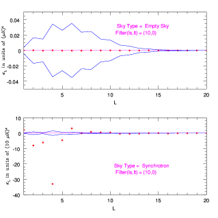
Figure 1: CMB polarization maps with no foregrounds are statistically isotropic and have null bipolar power spectrum (top). Adding polarized synchrotron emission violates statistical isotropy and results in a detectable non-zero bipolar power spectrum (bottom). Red dots show the BiPS after bias subtraction and Blue lines show the $1-\sigma$ of the cosmic variance.

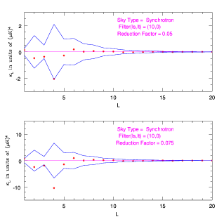
Figure 2: Adding $5\%$ of the polarized synchrotron emission just violates statistical isotropy (top). Adding $7.5\%$ of the polarized synchrotron emission clearly violates statistical isotropy and results in a detectable non-zero bipolar power spectrum (bottom). Red dots show the BiPS after bias subtraction and Blue lines show the $1-\sigma$ of the cosmic variance.

As an example of how one can detect deviations from statistical isotropy in CMB polarization maps, we make statistically anisotropic polarization maps and estimate the BiPS from them. This can be done in many different ways but here we choose a simple method which results in severe violation of SI and therefore is good for a demonstration of the method. We add polarized synchrotron emission template to the background CMB polarization map. Polarized synchrotron template $(30~{}GHz)$ is made using Planck Simulator plancksimulator which uses the model by Giardino:2002 , i.e. the polarization degree is a function of the intensity spectral index while polarization angles are derived from a gaussian distribution. Here we restrict our attention to $E$ mode polarization only. It is obvious that everything can be done in the same way for B mode as well. The estimator will then be

$$A^{EE}_{\ell M|ll^{\prime}}=\sum_{mm^{\prime}}\sqrt{W_{l}W_{l^{\prime}}}a^{E}_{lm}a^{E}_{l^{\prime}m^{\prime}}\,\,{\mathcal{C}}^{\ell M}_{lml^{\prime}m^{\prime}}\,\quad,$$ (24)

where $a^{E}_{lm}$ are the spherical harmonic transform of the background CMB polarization map plus the polarized synchrotron radiation,

$$a^{E}_{lm}=a^{E_{cmb}}_{lm}+a^{E_{sync}}_{lm}.$$ (25)

and $W_{l}$ is a isotropic filter that allows us to target angular scales of interest by filtering out power on other scales.

We simulate 1000 statistically isotropic CMB polarization maps, add the synchrotron template to each of them and compute the BiPS for them using the estimators of eqns. (24) and (22). Filters that we use here can be divided into two categories: low pass Gaussian filters

$$W_{l}^{G}=N^{G}\exp\left\{-\left(\frac{2l+1}{2l_{s}+1}\right)^{2}\right\}$$ (26)

that cuts power on scales, $l\leq l_{s}$ and band pass filters of the form

$$W_{l}^{S}=2N^{S}\left[1-J_{0}\left(\frac{2l+1}{2l_{s}+1}\right)\right]\exp\left\{-\left(\frac{2l+1}{2l_{s}+1}\right)^{2}\right\}\,,$$ (27)

that retains power on scales $l_{s}\leq l\leq l_{t}$, where $J_{0}$ is the spherical bessel function and $N^{G}$ and $N^{S}$ are normalization constants chosen such that, $\sum_{l}\frac{(2l+1)W_{l}}{2l(l+1)}=1$, i.e., unit rms for unit flat band angular power spectrum, $l(l+1)\,C^{XX^{\prime}}_{l}=2\pi$.

Results of this computation are shown in Fig. 1 and Fig. 2. We see that CMB polarization maps with no foregrounds are statistically isotropic and have null bipolar power spectrum. Adding polarized synchrotron emission violates statistical isotropy at large angular scales and results in a detectable non-zero BiPS. Retaining only $5\%$ of the polarized synchrotron emission just violates statistical isotropy at the threshold of $1-\sigma$. At $7.5\%$ of the polarized synchrotron emission clearly shows the violation of statistical isotropy and results in a sharply detectable non-zero bipolar power spectrum at $\kappa_{4}$.

We should emphasize that this is simply an example to demonstrate how violation of statistical isotropy can be quantified in CMB polarization maps. In reality, we usually expect to deal with cleaned polarized maps which would contain some residuals that have different angular structure. The signal would be much weaker and also have different BiPS characteristics. Hunting tiny residuals from foregrounds in maps of temperature anisotropy using statistical isotropy has been studied us_foregrounds and similar strategy can be applied to polarization maps when they are available. In addition, other observational artifacts such as anisotropic noise or incomplete (masked) sky can also cause violation of statistical isotropy in a polarization map. In the latter case, the incomplete sky coverage immediately induces a contamination of E-mode of polarization by its B-mode and vice-versa. Then the modified temperature and polarization fields is related to their actual values of full sky coverage by a window matrix Lewis:2002 ; Brown:2004 whose elements are basically window functions for temperature and polarization in harmonic space. It can be shown that the estimated BipoSH coefficients are in fact linear combinations of that for fullsky CMB maps.

$${\bf\tilde{A}}_{\ell M|ll^{\prime}}=\sum_{\ell^{\prime}M^{\prime}l_{1}l_{2}}{\bf N}^{\ell Mll^{\prime}}_{\ell^{\prime}M^{\prime}l_{1}l_{2}}\,\,{\bf A}_{\ell M|l_{1}l_{2}}\,.$$ (28)

Here bold-faced ${\bf\tilde{A}}_{\ell M|ll^{\prime}}$ and ${\bf A}_{\ell M|l_{1}l_{2}}$ are the column matrices corresponding to estimated and true BipoSH coefficients respectively, for the auto and cross-correlations $(TT,TE,TB,ET,EE,EB,BT,BE,BB)$ of temperature anisotropy and polarization. The elements of the matrix ${\bf N}^{\ell Mll^{\prime}}_{\ell^{\prime}M^{\prime}l_{1}l_{2}}$ depend on Clebsch- Gordan coefficients and window functions in harmonic space. Hence, the true BipoSH coefficients can be estimated from the pseudo-BipoSH coefficients by inverting the above equation. We defer this to a future publication, a SI analysis of CMB polarization when this effect is important. However, we have verified using simulations that the BiPS of polarization maps is insensitive to breakdown of SI due to galactic cut when it is filtered at low-l using, $W_{l}^{G}(l_{s}=10,l_{t}=0)$ and $W_{l}^{S}(l_{s}=20,l_{t}=10)$ in eqns.(26) & (27). (This is consistent with the result for cut-sky CMB temperature maps discussed in the paper us_bigpaper .) As a result, the BiPS signature of the polarized galctic foregrounds presented here would not change if the maps are masked by a galactic cut. CMB polarization maps filtered with windows peaked at higher multipoles (eg., $W_{l}^{S}(l_{s}=90,l_{t}=80)$) do reflect the SI violation arising from a galactic cut. The complications of quantifying statistical isotropy in cut-sky polarization CMB maps is formally encoded by eqn. (28) but its implementation is a challenging task which is currently under progress. (The effects can also be estimated through extensive simulations.)

VI Summary

We present a novel approach to quantify the violation of statistical isotropy in CMB polarization maps for the first time. We present a fast and orientation independent method which allows for a general test of isotropy using Bipolar Power Spectrum. This method has been previously applied to the temperature anisotropy maps and many various aspects of that are well studied in details. In this paper we extend BiPS to the CMB polarization maps and by present a working example to demonstrate its potential.

Appendix A Useful mathematical relations

Bipolar spherical harmonics form an orthonormal basis of $S^{2}\times S^{2}$ and are defined as

$$Y^{l_{1}l_{2}}_{\ell M}(\hat{n}_{1},\,\hat{n}_{2})\,=\,\sum_{m_{1}m_{2}}{\mathcal{C}}_{l_{1}m_{1}l_{2}m_{2}}^{\ell M}Y_{l_{1}m_{1}}(\hat{n}_{1})Y_{l_{2}m_{2}}(\hat{n}_{2}),$$ (29)

in which ${\mathcal{C}}_{l_{1}m_{1}l_{2}m_{2}}^{\ell M}$ are Clebsch-Gordan coefficients. Clebsch-Gordan coefficients are non-zero only if triangularity relation holds, $\{l_{1}l_{2}\ell\}$, and $M=m_{1}+m_{2}$. Where the $3j$-symbol $\{abc\}$ is defined by

$$\{abc\}=\left\{\begin{array}[]{ll}1&\textrm{if $a+b+c$ is integer and $|a-b|\leq c\leq(a+b)$,}\\ 0&\textrm{otherwise,}\end{array}\right.$$

Orthonormality of bipolar spherical harmonics

$$\int d\Omega_{\hat{n}_{1}}d\Omega_{\hat{n}_{2}}\,Y^{l_{1}l_{2}}_{\ell M}(\hat{n}_{1},\,\hat{n}_{2})Y^{*l^{\prime}_{1}l^{\prime}_{2}}_{\ell^{\prime}M^{\prime}}(\hat{n}_{1},\,\hat{n}_{2})=\delta_{l_{1}l^{\prime}_{1}}\delta_{l_{2}l^{\prime}_{2}}\delta_{\ell\ell^{\prime}}\delta_{MM^{\prime}}$$ (30)

References

- (1) A. Hajian and T. Souradeep, 2003b, ApJ 597, L5 (2003).
- (2) T. Souradeep and A. Hajian, Pramana 62 (2004) 793-796.
- (3) T. Souradeep and A. Hajian, Proceedings of JGRG-14, (2004).
- (4) M. Zaldarriaga and U. Seljak, Phys. Rev. D 55, 1830(1997).
- (5) M. Kamionkowski, A. Kosowsky and A. Stebbins, Phys. Rev. D 55, 7368 (1997).
- (6) A. Lewis, A. Challinor, N. Turok, 2002, Phys. Rev. D, 65, 023505.
- (7) M. L. Brown, P. G. Castro, A. N. Taylor, Mon.Not.Roy.Astron.Soc. 360, 1262-1280, (2005).
- (8) N. Bartolo, E. Komatsu, S. Matarrese and A. Riotto, Phys. Rept. 402, 103 (2004).
- (9) E. Komatsu et al., Astrophys. J. Suppl. 148, 119 (2003).
- (10) D. A. Varshalovich, A. N. Moskalev and V. K. Kher- sonskii, 1988 Quantum Theory of Angular Momentum (World Scientific).
- (11) A. Hajian and T. Souradeep, 2005, preprint. (astro-ph/0501001).
- (12) Amir Hajian, Tarun Souradeep and Neil J. Cornish, Astrophys.J. 618, L63 (2004).
- (13) http://www.g-vo.org/planck/
- (14) G. Giardino, A. J. Banday, K. M. Gorski, K. Bennett, J. L. Jonas and J. Tauber, arXiv:astro-ph/0202520.
- (15) R. Saha, A. Hajian, T. Souradeep and P. Jain, 2006, in preparation.