On the mean field dynamo with Hall effect

Abstract

Context. MHD turbulence with Hall effect.

Aims. Study how Hall effect modifies the quenching process of the electromotive force (e.m.f.) in Mean Field Dynamo (MFD) theories.

Methods. We write down the evolution equations for the e.m.f. and for the large and small scale magnetic helicity, treat Hall effect as a perturbation and integrate the resulting equations, assuming boundary conditions such that the total divergencies vanish.

Results. For force-free large scale magnetic fields, Hall effect acts by coupling the small scale velocity and magnetic fields. For the range of parameters considered, the overall effect is a stronger quenching of the e.m.f. than in standard MHD and a damping of the inverse cascade of magnetic helicity.

Conclusions. In astrophysical environments characterized by the parameters considered here, Hall effect would produce an earlier quenching of the e.m.f. and consequently a weaker large scale magnetic field.

1 Introduction

The origin and evolution of magnetic fields observed in all objects of the universe is one of the main problems in astrophysics. The basic physical process assumed to create them is a dynamo, which needs two basic ingredients, a seed field and an amplifying mechanism, each of them constituting at present an independent line of research (e.g., Grasso & Rubinstein rev-dg (2001), Widrow rev-lw (2002), Giovannini rev-mg (2004)). An amplifying mechanism usually considered is the so called turbulent Mean Field Dynamo (MFD), as turbulence is normally present in astrophysical environments. In this mechanism it is assumed that turbulence is excited at a small scale $\ell_{s}$ and that as a consequence a magnetic field is induced at a larger scale $\ell_{L}$. This theory has been a useful framework for modeling local origin of large scale magnetic fields in stars and galaxies.

In the Universe there are very different astrophysical environments: compact stars, low density and low temperature plasmas, accretion disks around stars and in AGN’s, etc. The plasma in each of those ambients has a different composition and therefore different physical processes may be relevant: in low ionized plasmas as the interstellar medium, ambipolar difussion is important (Zweibel zweibel (1988)); in the high-temperature intracluster gas ohmic dissipation plays a major role, and Hall effect can be relevant in accretion disks (Sano & Stone stone (2002), Wardle wardle99 (1999), Balbus & Terquem balb-terq (2001)) as well as in the early universe (Tajima et al. tajima (1992)). Turbulent dynamo operation may therefore be affected by the composition of the plasma: if we consider a plasma formed by, e.g. protons, electrons and neutrals, then the different interactions among these constituents can be expressed as a generalized Ohm’s law (Spitzer spitzer (1962), Priest priest (1982)).

One of the main steps in the development of a turbulent mean field (or large scale) dynamo theory was the recognition of the pivotal role played by magnetic helicity (e.g., Pouquet et al. pfl (1976), Blackman & Field 2001a ; 2001b , Brandenburg bran-2001 (2001)). In the absence of resistive dissipation, and for boundary conditions such that total divergencies vanish, this quantity is globally conserved, independently of any assumption about the turbulent state of the system. Its evolution does not explicitly depend on the non-linear backreaction due to Lorentz force, it merely depends on the induction equation, providing therefore a strong constraint on the nonlinear evolution of the large scale magnetic field.

As stated above, mean field dynamo amounts to split the fields into large scale mean fields ${\bf U}_{0}$, ${\bf B}_{0}$, ${\bf A}_{0}$ and small scale turbulent fields ${\bf u}$, ${\bf b}$, ${\bf a}$. This small scale fields represent the “waste product” of turbulence, and they can be very intense in spite of their small coherence length . In this theory the evolution equation for ${\bf B}_{0}$ can be cast as $\partial{\bf B}_{0}/\partial t={\bf\nabla}\times\left({\bf U}_{0}\times{\bf B}_{0}+{\bf\varepsilon}-\eta{\bf J}_{0}\right)$, where ${\bf J}_{0}$ is the mean electric current, $\eta$ the resisitivity and ${\bf\varepsilon}=\langle{\bf u}\times{\bf b}\rangle_{0}$ the turbulent electromotive force (e.m.f.). In the two scale approach it is assumed that ${\bf\varepsilon}$ can be expanded in powers of the gradients of ${\bf B}_{0}$ in the rather general form $\varepsilon_{i}=\alpha_{ij}\left(\hat{\bf g},\hat{\bf\Omega},{\bf B}_{0},...\right)B_{0j}+\eta_{ijk}\left(\hat{\bf g},\hat{\bf\Omega},{\bf B}_{0},...\right)\partial B_{0j}/\partial x_{k}$, where the functions $\alpha_{ij}$ and $\eta_{ijk}$ are called turbulent transport coefficients. They depend on the stratification $\hat{\bf g}$, angular velocity $\hat{\bf\Omega}$ and mean magnetic field ${\bf B}_{0}$.They may also depend on correlators involving the small scale magnetic field in the form, for example, of small scale current helicity.

The simplest way of calculating the turbulent transport coefficients consists of linearizing the equations for the small scale quantities, ignoring quadratic terms that would lead to triple correlations in the expressions for the quadratic terms. In other words, the backreaction of mean field ${\bf B}_{0}$ on the correlation tensor of the turbulence is taken into account, while neglecting the effect of the small scale fields. In this way the electromotive force can be written as (Krause & Rädler krause (1980)) ${\bf\varepsilon}=\alpha{\bf B}_{0}-\beta{\bf J}_{0}$ with $\alpha\simeq-(1/3)\tau_{corr}\langle{\bf u}\cdot{\bf\nabla}\times{\bf u}\rangle_{0}$ and $\beta\simeq(1/3)\tau_{corr}\langle u^{2}\rangle_{0}$, with $\tau_{corr}$ the correlation time. These modifications of the turbulent transport coefficients have been calculated about thirty years ago, and the approximation is known as First order smoothing approximation, or FOSA (see also Moffat moffat2 (1972), Rüdiger rudiger (1974) Parker parker (1955); Moffat moffat (1978); Zel’dovich, Ruzmaikin & Sokoloff zeldovich (1983)).

There remains to incorporate the modifications to ${\bf\varepsilon}$ that involve the small scale, fluctuating fields. They arise when calculating $\langle{\bf u}\times{\bf b}\rangle_{0}$ from terms involving the nonlinear terms and the Lorentz force in the evolution equations for ${\bf b}$ and ${\bf u}$ respectively. As a consequence, the $\alpha$ term written above gets renormalized in the nonlinear regime by the addition of a term proportional to the current helicity $\langle{\bf b}\cdot\left({\bf\nabla}\times{\bf b}\right)$ of the fluctuating field, which in turn is related to the magnetic helicity of the small scale magnetic field. The $\beta$ term on the other side is not affected by the backreaction of the small scale fields (Pouquet et all pfl (1976), Subramanian & Brandenburg sub-bran (2004), Brandemburg & Subramanian report-bs (2005)). In this way we have $\alpha\simeq-(1/3)\tau_{corr}\left(\langle{\bf u}\cdot\left({\bf\nabla}\times{\bf u}\right)\rangle_{0}-\langle{\bf b}\cdot\left({\bf\nabla}\times{\bf b}\right)\rangle_{0}\right)$.

In this paper we investigate how Hall effect modifies the process of quenching of the e.m.f. ${\bf\varepsilon}$, described in the previous paragraphs. For this purpose we use a closure scheme recently introduced by Blackman & Field (fb2002-2 (2002, 2004)), that permits to study dinamically the backreaction of both the large and small scale fields on ${\bf\varepsilon}$. This closure, also named the “minimal $\tau$ approximation”, consists in finding the evolution equation for the electromotive force instead of finding ${\bf\varepsilon}$ itself. In it, three point correlations of the generated small scale fields, $\bar{\bf T}$, are not neglected, but their sum is assumed to be a negative multiple of the second order correlator, i.e. $\bar{\bf T}=-{\bf\varepsilon}/\tau$. This assumption produces results that are in very good agreement with numerical simulations (Brandenburg & Subramanian report-bs (2005)).

Hall effect is taken into account by considering a corresponding term in Ohm’s law (see Spitzer spitzer (1962), Priest priest (1982)). The parameter that meassures its intensity is the Hall length, that in alfvénic units is defined as $\ell_{H}=\left(4\pi\rho\right)^{1/2}/n_{e}e$, with $\rho$ the mass density and $n_{e}$ the electronic numerical density. Of interest is the ratio of this length, to the Ohmic dissipation length, $\ell_{\eta}$, and to the scale of the flow, $\ell_{u}$. For $\ell_{H}\lesssim l_{\eta}$, the Hall-MHD equations reduce to those of standard MHD, as ohmic dissipation erases any other interaction. In several astrophysical problems, such as accretion disks, protoplanetary disks, the early universe plasma and the magnetopause (Birn et al birn (2001), Balbus & Terquem balb-terq (2001), Sano & Stone stone (2002), Tajima et al tajima (1992)), the Hall scale is larger than the Ohmic scale, but it can be smaller or larger than $\ell_{u}$.

Under the hypothesis that large scale fields are force-free (which is a reasonable assumption in many astrophysical environments) we obtain evolution equations for the mean magnetic field and for the large and small scale magnetic helicities, that are formally identical to those obtained in absence of Hall effect, provided that we redefine the electromotive force by ${\bf\varepsilon}_{H}=\langle{\bf u}_{e}\times{\bf b}\rangle$ with $u_{e}=u-\ell_{H}\langle\left({\bf\nabla}\times{\bf b}\right)\times{\bf b}\rangle_{0}$. This means that the component of ${\bf\varepsilon}_{H}$ along the mean field ${\bf B}_{0}$ governs the evolution of magnetic helicity, and in turn magnetic helicity influences the growth of ${\bf B}_{0}$ ( Parker parker (1955), Ji ji-99 (1999)). We study a system of coupled evolution equations for ${\bf\varepsilon}_{H}$ and for the large and small scale magnetic helicities. As mentioned above, the evolution equations for the helicities are formally identical to the ones in absence of Hall effect. In contrast, the equation for ${\bf\varepsilon}_{H}$ presents substantial differences in comparison to the standard MHD case: (i) In the $\alpha$ term, proportional to ${\bf B}_{0}$, the fluid helicity is replaced by the electronic fluid helicity and there appears an extra term, explicitly dependent on $\ell_{H}$ that couples ${\bf b}$ with ${\bf u}_{e}$. (ii) In the turbulent diffusion term, proportional to ${\bf\nabla}\times{\bf B}_{0}$, the $\beta$ term, the fluid kinetic energy term $\langle u^{2}\rangle_{)}$ is replaced by $\langle{\bf u}\cdot{\bf u}_{e}\rangle_{0}$ and there also appears a correction explicitly dependent on $\ell_{H}$, that couples ${\bf b}$ with ${\bf u}$. All these modifications render this term not positive definite, a fact that could produce a transfer of energy from small scales toward large scales or, in other words an inverse cascade of energy (Mininni et al. pablito4 (2005)). (iii) There appears a new term, proportional to $\nabla^{2}{\bf B}_{0}$, that again couples the mentioned velocities. The coupling of ${\bf u}_{e}$ with ${\bf b}$ indicates that Hall effect acts by transferring energy between these two fields in a non-trivial way.

In order to illustrate how Hall effect affects the quenching process of the mean field dynamo, we applied the obtained equations to a specific physical situation in which we considered that turbulence of maximal kinetic helicity is excited at a certain scale $\ell_{s}$ and that the large scale magnetic field is generated at a scale $\ell_{L}=5\ell_{s}$. As for the Hall effect, we considered $\ell_{s}<\ell_{H}<\ell_{L}$ and treated it as a perturbation. We find that for this situation the overall effect is a quenching of the e.m.f. stronger than in standard MHD, acompanied by a supression of magnetic helicity inverse cascade. Our results are in qualitative agreement with recent numerical simulations performed by Mininni et al (2003b ).

As the aim of this paper is to understand conceptually how Hall effect acts on a MFD, we did not apply our results to a concrete astrophysical object. We leave this issue for future work, after a deeper understanding of the mechanism is attained. The paper is organized as follows: in section §2 we present the main equations and deduce the evolution equations for large and small scale fields. In section §3 we deduce the dynamo equations, i.e., the ones for the stochastic electromotive force and for the large and small scale magnetic helicities. In section §4 we implement a two scale approximation and numerically integrate the system of equations and discuss the results. Finally in section §5 we sumarize our conclusions.

2 Main Equations

In Magnetohydrodynamics, Hall effect can be taken into account through the generalized Ohm’s law as (e.g., Spitzer spitzer (1962), Priest priest (1982)):

$${\bf E}+{\bf U}\times{\bf B}=\frac{1}{n_{e}e}{\bf J}\times{\bf B}+\eta{\bf\nabla}\times{\bf B}\,,$$ (1)

with ${\bf J}={\bf\nabla}\times{\bf B}$, $n_{e}$ the electron number density, $e$ the modulus of the fundamental electric charge and $\eta$ the Ohmic diffusion coefficient. We need the magnetic field induction and the Navier Stokes equations. We use units in which the magnetic field has dimensions of velocity. To simplify the calculations and the comparison with previous works we shall consider an incompressible fluid, i.e., $\nabla\cdot{\bf U}=0$. This condition is fulfilled in several astrophysical environments. The Navier-Stokes equation is then written as:

$$\frac{\partial{\bf U}}{\partial t}=-{\bf\bar{P}}\left[\left({\bf U}\cdot{\bf\nabla}\right){\bf U}-\left({\bf B}\cdot{\bf\nabla}\right){\bf B}\right]-\nu{\bf\nabla}\times\left({\bf\nabla}\times{\bf U}\right)\,,$$ (2)

where ${\bf\bar{P}}\equiv{\bf I}-{{\bf\nabla}{\bf\nabla}\cdot}/{\nabla^{2}}$ is the projector operator onto the subspace of solutions of this equation that satisfy the condition of incompressibility (McComb macomb (2003)) and $\nu$ the kinematic viscosity. The induction equation reads:

$$\frac{\partial{\bf B}}{\partial t}={\bf\nabla}\times\left\{{\bf U}\times{\bf B}-\ell_{H}\left({\bf\nabla}\times{\bf B}\right)\times{\bf B}-\eta{\bf\nabla}\times{\bf B}\right\}\,,$$ (3)

where we defined the Hall length, $\ell_{H}$, as $\ell_{H}={\left(4\pi\rho\right)^{1/2}}/{n_{e}e}$. We also need the equation for the vector potential ${\bf A}$. If we choose to work with the Coulomb gauge, i.e., ${\bf\nabla}\cdot{\bf A}=0$, it reads:

$$\frac{\partial{\bf A}}{\partial t}={\bf\bar{P}}\left[{\bf U}\times{\bf B}-\ell_{H}\left({\bf\nabla}\times{\bf B}\right)\times{\bf B}\right]-\eta{\bf\nabla}\times{\bf B}\,,$$ (4)

where ${\bf\bar{P}}$ is the previously defined projector, but now projecting onto the space of functions that satisfy the chosen gauge. When $\eta=0$, Equation (3) represents the freezing of the magnetic field to the electron flux. To see this, let us write ${\bf U}_{e}={\bf U}-\ell_{H}{\bf\nabla}\times{\bf B}$, which when substituted in eqs (3) and (4) transforms them in equations formally identical to the ones without Hall effect.

2.1 Large and Small Scale Fields

As we are interested in studying mean field dynamo, we split the fields ${\bf U}$, ${\bf B}$ and ${\bf A}$ as ${\bf U}={\bf u}$, ${\bf B}={\bf B}_{0}+{\bf b}$ and ${\bf A}={\bf A}_{0}+{\bf a}$. Upper case and subindex $0$ denote large scale fields, i.e. vector quantities whose value may vary in space but whose direction and sense are almost uniform or vary very smoothly. Technically speaking, they represent local spatial averages. Lowercase denotes small scale, stochastic fields, i.e. fields whose amplitude may be large, but that have a very small coherence length. We assume that any average of stochastic quantities is zero. Observe that we assumed ${\bf U}_{0}=0$, i.e. no large scale flows.

2.1.1 Evolution equation for the mean fields

To derive the evolution equations for the large scale fields, we replace the previous decomposition into eqs. (3) and (4) and take local spatial averages that we denote as $\langle...\rangle_{0}$ . If besides we demand large scale fields to be force-free, we obtain:

$$\frac{\partial{\bf B}_{0}}{\partial t}={\bf\nabla}\times{\bf\varepsilon}_{H}+\eta\nabla^{2}{\bf B}_{0}\,,$$ (5)

$$\frac{\partial{\bf A}_{0}}{\partial t}={\bf\bar{P}}{\bf\varepsilon}_{H}+\eta\nabla^{2}{\bf A}_{0}\,,$$ (6)

where with the aid of Reynolds rules (McComb macomb (2003)) we have interchanged derivatives with averages. We have also defined a Hall turbulent electromotive force as:

$${\bf\varepsilon}_{H}=\langle{\bf u}\times{\bf b}\rangle_{0}-\ell_{H}\langle\left({\bf\nabla}\times{\bf b}\right)\times{\bf b}\rangle_{0}\equiv\langle{\bf u}_{e}\times{\bf b}\rangle_{0}\,.$$ (7)

2.1.2 Evolution equations for the small scale fields

The evolution equations for the small scale fields are obtained by replacing the decomposition of fields into global averages and stochastic component, into eqs. (2), (3) and (4) and substracting from them the equations for the mean fields. Thus we have:

$$\frac{\partial{\bf u}}{\partial t} = {\bf\bar{P}}\left[\left({\bf b}\cdot{\bf\nabla}\right){\bf B}_{0}+\left({\bf B}_{0}\cdot{\bf\nabla}\right){\bf b}\right]+{\bf\bar{P}}\left[\left({\bf b}\cdot{\bf\nabla}\right){\bf b}-\left({\bf u}\cdot{\bf\nabla}\right){\bf u}\right]$$ (8)

$$- \nu{\bf\nabla}\times\left({\bf\nabla}\times{\bf u}\right)\,,\leavevmode\nobreak\ \leavevmode\nobreak\ \leavevmode\nobreak\ \leavevmode\nobreak\ \leavevmode\nobreak\ \leavevmode\nobreak\ \leavevmode\nobreak\ \leavevmode\nobreak\ \leavevmode\nobreak\ \leavevmode\nobreak\ \leavevmode\nobreak\ \leavevmode\nobreak\ \leavevmode\nobreak\ \leavevmode\nobreak\ \leavevmode\nobreak\ \leavevmode\nobreak\ \leavevmode\nobreak\ \leavevmode\nobreak\ \leavevmode\nobreak\ \leavevmode\nobreak\ \leavevmode\nobreak\ \leavevmode\nobreak\ \leavevmode\nobreak\ \leavevmode\nobreak\ \leavevmode\nobreak\ \leavevmode\nobreak\ \leavevmode\nobreak\ \leavevmode\nobreak\ \leavevmode\nobreak\ \leavevmode\nobreak\ \leavevmode\nobreak\ \leavevmode\nobreak\ \leavevmode\nobreak\ \leavevmode\nobreak\ \leavevmode\nobreak\ \leavevmode\nobreak\ \leavevmode\nobreak\ \leavevmode\nobreak\ \leavevmode\nobreak\ \leavevmode\nobreak\ \leavevmode\nobreak\ \leavevmode\nobreak\ \leavevmode\nobreak\ \leavevmode\nobreak\ \leavevmode\nobreak\ \leavevmode\nobreak\ \leavevmode\nobreak\ \leavevmode\nobreak\ \leavevmode\nobreak\ \leavevmode\nobreak\ \leavevmode\nobreak\ \leavevmode\nobreak\ \leavevmode\nobreak\ \leavevmode\nobreak\ \leavevmode\nobreak\ \leavevmode\nobreak\ \leavevmode\nobreak\ \leavevmode\nobreak\$$

$$\frac{\partial{\bf b}}{\partial t} = {\bf\nabla}\times\left({\bf u}_{e}\times{\bf B}_{0}\right)-\ell_{H}{\bf\nabla}\times\left[\left({\bf\nabla}\times{\bf B}_{0}\right)\times{\bf b}\right]+{\bf\nabla}\times\left({\bf u}_{e}\times{\bf b}\right)$$ (9)

$$- \langle{\bf\nabla}\times\left({\bf u}_{e}\times{\bf b}\right)\rangle_{0}-\eta{\bf\nabla}\times\left({\bf\nabla}\times{\bf b}\right)\,,$$

and:

$$\frac{\partial{\bf a}}{\partial t} = {\bf\bar{P}}\left({\bf u}_{e}\times{\bf B}_{0}\right)-\ell_{H}{\bf\bar{P}}\left[\left({\bf\nabla}\times{\bf B}_{0}\right)\times{\bf b}\right]+{\bf\bar{P}}\left({\bf u}_{e}\times{\bf b}\right)$$ (10)

$$- \langle{\bf\bar{P}}\left({\bf u}_{e}\times{\bf b}\right)\rangle_{0}-\eta{\bf\nabla}\times\left({\bf\nabla}\times{\bf a}\right)\,.$$

3 Dynamo equations

Now that we have the complete set of evolution equations for large and small scale quantities, we can proceed to derive the evolution equations for the electromotive force and the magnetic helicity.

3.1 Magnetic helicity evolution equation

Magnetic helicity is defined as the global average, or average over the entire volume of ${\bf A}\cdot{\bf B}$, that we denote by $H^{M}_{T}=\langle{\bf A}\cdot{\bf B}\rangle_{vol}$ (Biskamp biskamp (1997)). These quantities do not vary in space, they depend only on time. Call $H^{M}\equiv\langle{\bf A}_{0}\cdot{\bf B}_{0}\rangle_{vol}$ and $h^{M}\equiv\langle{\bf a}\cdot{\bf b}\rangle_{vol}$. By taking the time derivative of these quantities with respect to time and using eqs. (3), (4), (9) and (10) we obtain

$$\frac{\partial H^{M}}{\partial t} = 2\langle{\bf\varepsilon}_{H}\cdot{\bf B}_{0}\rangle_{vol}-2\eta\langle{\bf B}_{0}\cdot\left({\bf\nabla}\times{\bf B}_{0}\right)\rangle_{vol}$$ (11)

$$+ \langle{\bf\nabla}\cdot\left[{\bf\varepsilon}_{H}\times{\bf A}_{0}-\eta\left({\bf\nabla}\times{\bf B}_{0}\right)\times{\bf A}_{0}\right]\rangle_{vol}\,,$$

and:

$$\frac{\partial h^{M}}{\partial t} = -2\langle{\bf\varepsilon}_{H}\cdot{\bf B}_{0}\rangle_{vol}-2\eta\langle\langle\left({\bf\nabla}\times{\bf b}\right)\cdot{\bf b}\rangle_{0}\rangle_{vol}$$ (12)

$$+ \langle{\bf\nabla}\cdot\left\{\left[{\bf u}_{e}\times{\bf B}_{0}-\ell_{H}\left({\bf\nabla}\times{\bf B}_{0}\right)\times{\bf b}\right]\times{\bf a}\right\}\rangle_{vol}$$

$$+ \langle{\bf\nabla}\cdot\left\{\left[{\bf u}_{e}\times{\bf b}-\eta{\bf\nabla}\times{\bf b}\right]\times{\bf a}\right\}\rangle_{vol}\,,$$

To deal with the operator ${\bf\bar{P}}$ we followed the procedure deviced by Gruzinov & Diamond (gruzinov-2 (1995)), that consists in transforming Fourier the equations before taking averages, and make a development to first order in $k_{L}/k_{s}$ with $k_{L}$ the scale of $B_{0}$ and $k_{s}$ the scale of the small scale fields. We also made some simple algebraic manipulation to put the total divergencies in evidence. If we add up eqs (11) and (12) we see that total magnetic helicity is conserved, except for the divergencies and the dissipative terms. This means that the term $\langle{\bf\varepsilon}_{H}\cdot{\bf B}_{0}\rangle_{vol}$ transforms magnetic helicity between mean and fluctuating fields. In what follows we consider boundary conditions such that the divergencies in eqs. (11) and (12) vanish. This selection is debatable, however, in view of the fact that such conditions may not be quite general, or easily attainable in practice. Nevertheless they have two advantages: First, the resulting magnetic helicity is gauge invariant and second, they are widely used in numerical simulations, a fact that will facilitate comparisons with those works. The effect of boundary conditions on the evolution and gauge invariance of magnetic helicity is discussed in Berger & Field (berger (1984)), Ji (ji-99 (1999)), Vishniac & Cho (vish-cho (2001)), and Subramanian & Brandenburg (sub-bran (2004)).

3.2 Evolution equation for ${\bf\varepsilon}_{H}^{\parallel}$

According to its definition, eq. (7), ${\bf\varepsilon}_{H}$ is the combination of two terms. So we need to find evolution equations for each term and then join them into one equation. The derivation is sketched in Appendix A, eq. (27), and here we quote the final result, namely:

$$\frac{\partial{\bf\varepsilon}_{H}}{\partial t} = \frac{1}{3}\left\{-\langle{\bf u}_{e}\cdot\left({\bf\nabla}\times{\bf u}_{e}\right)\rangle_{0}+\langle\left({\bf\nabla}\times{\bf b}\right)\cdot{\bf b}\rangle_{0}+\ell_{H}\langle{\bf b}\cdot\nabla^{2}{\bf u}_{e}\rangle_{0}\right\}{\bf B}_{0}$$ (13)

$$- \frac{1}{3}\left[\langle{\bf u}\cdot{\bf u}_{e}\rangle_{0}+\ell_{H}\langle{\bf b}\cdot\left({\bf\nabla}\times{\bf u}\right)\rangle_{0}\right]\left({\bf\nabla}\times{\bf B}_{0}\right)$$

$$+ \frac{1}{3}\ell_{H}\langle{\bf u}_{e}\cdot{\bf b}\rangle_{0}\nabla^{2}{\bf B}_{0}$$

$$+ \eta\left[\langle{\bf u}_{e}\times\nabla^{2}{\bf b}\rangle_{0}-\ell_{H}\langle\left({\bf\nabla}\times\nabla^{2}{\bf b}\right)\times{\bf b}\rangle_{0}\right]$$

$$+ \nu\langle\nabla^{2}{\bf u}\times{\bf b}\rangle_{0}+{\bf\bar{T}}\,,$$

with ${\bf\bar{T}}$ representing the small scale field, three-point correlations and given in Appendix A by eq. (26). The term proportional to ${\bf B}_{0}$ is similar to the “$\alpha$” term that appears in the kinematic dynamo, except that now it has the electronic kinetic helicity ($1^{st}$ term inside braces) instead of the fluid kinetic helicity of the ordinary dynamo. Besides this term, there is a current helicity term ($2^{nd}$ term inside braces, also present in standard MHD dynamo equation) that is due to the small scale magnetic field and that can be cast in terms of the small scale magnetic helicity. Finally there is a new term that is an explicit Hall modification ($3^{rd}$ term in braces), that couples the small scale magnetic field to the electronic velocity field.

The term proportional to $\left({\bf\nabla}\times{\bf B}_{0}\right)$, named “$\beta$ term” is also strongly modified: the first term turns out to be the scalar product of the fluid and kinetic velocities, and there appears a second term, explicitly dependent on $\ell_{H}$ that couples ${\bf u}$ to ${\bf b}$. All these modifications made this term not positive definite anymore. A negative value of this coefficient represents non-local transfer from small scale turbulent fields to the large scale magnetic field (Mininni et al pablito4 (2005)). Finally there appears a new term, proportional to $\nabla^{2}{\bf B}_{0}$.

From eqs. (11) and (12) we see that the important quantity in the mean field dynamo operation is the component of ${\bf\varepsilon}_{H}$ parallel to ${\bf B}_{0}$ (Parker parker (1955)), which can be written as ${\bf\varepsilon}_{H}^{\parallel}={\bf\varepsilon}_{H}\cdot{\bf B}_{0}/|{\bf B}_{0}|$ and whose evolution equation is then given by ${\partial{\bf\varepsilon}_{H}^{\parallel}}/{\partial t}=\left({\partial{\bf\varepsilon}_{H}}/{\partial t}\right)\left({{\bf B}_{0}}/{|{\bf B}_{0}|}\right)+{\bf\varepsilon}_{H}\left[\partial\left({\bf B}_{0}/|{\bf B}_{0}|\right)/{\partial t}\right]$. To numerically integrate the resulting equation it is more convenient to write ${\bf u}_{e}$ back in terms of ${\bf u}$ and ${\bf b}$. The physical reason is that ${\bf u}$ is the velocity that can be externally excited or prescribed. Thus we shall work with (see eq. 25 of Appendix.)

$$\frac{\partial{\bf\varepsilon}_{H}^{\parallel}}{\partial t} = \frac{1}{3}\left\{\langle\left({\bf\nabla}\times{\bf b}\right)\cdot{\bf b}\rangle_{0}-\langle{\bf u}\cdot\left({\bf\nabla}\times{\bf u}\right)\rangle_{0}-\ell_{H}\langle{\bf u}\cdot\nabla^{2}{\bf b}\rangle_{0}\right.$$ (14)

$$+ \ell_{H}\langle{\bf b}\cdot\nabla^{2}{\bf u}\rangle_{0}+\ell_{H}\langle\left({\bf\nabla}\times{\bf b}\right)\cdot\left({\bf\nabla}\times{\bf u}\right)\rangle_{0}$$

$$- \ell_{H}^{2}\langle{\bf b}\cdot\left[{\bf\nabla}\times\nabla^{2}{\bf b}\right]\rangle_{0}+\ell_{H}^{2}\langle\left({\bf\nabla}\times{\bf b}\right)\cdot\nabla^{2}{\bf b}\rangle_{0}\left.\right\}|{\bf B}_{0}|$$

$$- \frac{1}{3}\left[\langle v^{2}\rangle_{0}+\ell_{H}\langle{\bf\nabla}\cdot\left({\bf u}\times{\bf b}\right)\rangle_{0}\right]\frac{\left({\bf\nabla}\times{\bf B}_{0}\right)\cdot{\bf B}_{0}}{|{\bf B}_{0}|}$$

$$+ \frac{1}{3}\ell_{H}\left[\langle{\bf u}\cdot{\bf b}\rangle_{0}-\ell_{H}\langle\left({\bf\nabla}\times{\bf b}\right)\cdot{\bf b}\rangle_{0}\right]\frac{\left(\nabla^{2}{\bf B}_{0}\right)\cdot{\bf B}_{0}}{|{\bf B}_{0}|}$$

$$- \zeta_{H}^{\parallel}{\bf\varepsilon}_{H}^{\parallel}\,.$$

where the last term represents the dissipative terms and the more important the three-point correlations of the generated small scale fields.

4 Solving the System

4.1 Further approximations and numerical integration

To numerically integrate the equations, we assume that full helical turbulence is excited at a certain scale $\ell_{S}$ smaller than the system’s size, and that the large scale magnetic field is induced at a larger scale $\ell_{L}=5\ell_{s}$, that can be the system’s size. This assumption enables us to consider that spectra of small scale quantities peak at wavenumber $k_{S}=2\pi/\ell_{S}$ while large scale quantities do so at $k_{L}=2\pi/\ell_{L}$. This assumption in based on the work of Pouquet, Frish & Leorat (pfl (1976)), who several years ago showed that when helical turbulence is induced at the scale $k_{s}$, large scale quantities peaked at a smaller $k_{L}$ (see also Maron & Blackman maron (2002)). Therefore we write the different terms of equations (11), (12) and (14) as: $\langle{\bf a.b}\rangle_{vol}=h^{M}_{s}$, $\langle{\bf A}_{0}.{\bf B}_{0}\rangle_{vol}=H^{M}_{L}$, $\langle{\bf u.b}\rangle_{vol}=h^{C}$, $\langle{\bf b}.\left({\bf\nabla}\times{\bf b}\right)\rangle_{0}=k_{S}^{2}h^{M}_{s}$, $\langle{\bf u}.\left({\bf\nabla}\times{\bf u}\right)\rangle_{0}=h^{u}$, $\langle{\bf u}.\nabla^{2}{\bf b}\rangle_{0}=-k_{S}^{2}h^{C}$, $\langle{\bf b}.\nabla^{2}{\bf u}\rangle_{0}=-k_{S}^{2}h^{C}$, $\langle\left({\bf\nabla}\times{\bf b}\right).\left({\bf\nabla}\times{\bf u}\right)\rangle_{0}=k_{S}^{2}h^{C}$, $\langle\left({\bf\nabla}\times{\bf b}\right).\nabla^{2}{\bf b}\rangle_{0}=-k_{S}^{4}h^{M}_{s}$, $\langle{\bf b}.\left({\bf\nabla}\times\nabla^{2}{\bf b}\right)\rangle_{0}=-k_{S}^{4}h^{M}_{s}$, $\langle{\bf\nabla}\cdot\left({\bf u}\times{\bf b}\right)\rangle_{0}=\pm k_{S}|\varepsilon_{0}|$, $\nabla^{2}{\bf B}_{0}=-k_{L}^{2}{\bf B}_{0}$. Besides we write $\langle{\bf u.u}\rangle_{0}=2e^{u}$. We see that in this case the the interaction between ${\bf u}$ and ${\bf b}$ is described by the small scale cross-helicity $\langle{\bf u}\cdot{\bf b}\rangle_{0}\equiv h^{C}$. For ${\bf B}_{0}$, as it is force-fee, we have $|{\bf B}_{0}|=k_{L}^{1/2}|h^{M}_{L}|^{1/2}$, and $\left({\bf\nabla}\times{\bf B}_{)}\right).{\bf B}_{0}=k_{L}^{2}h^{M}_{L}$. When we replace these expressions in eqs. (11) and (12) and (14) we obtain:

$$\frac{\partial\varepsilon_{H}^{\parallel}}{\partial t} = \frac{1}{3}\left\{k_{S}^{2}h^{M}_{s}-h^{u}+\ell_{H}k_{S}^{2}h^{C}\right\}k_{L}^{1/2}|h^{M}_{L}|^{1/2}$$ (15)

$$- \frac{2}{3}\left(e^{u}\pm\ell_{H}k_{S}|\varepsilon_{0}|\right)k_{L}^{3/2}\frac{h^{M}_{L}}{|h^{M}_{L}|^{1/2}}$$

$$- \frac{\ell_{H}}{3}\left[h^{C}-\ell_{H}k_{s}^{2}h^{M}_{s}\right]k_{L}^{5/2}|h^{M}_{L}|^{1/2}-\zeta_{H}^{\parallel}{\bf\varepsilon}_{H}^{\parallel}\,,$$

$$\frac{\partial}{\partial t}h^{M}_{L}=2k_{L}^{1/2}\varepsilon_{H}^{\parallel}|h^{M}_{L}|^{1/2}-2\eta k_{L}^{2}h^{M}_{L}\,$$ (16)

and

$$\frac{\partial}{\partial t}h^{M}_{s}=-2k_{L}^{1/2}\varepsilon_{H}^{\parallel}|h^{M}_{L}|^{1/2}-2\eta k_{s}^{2}h^{M}_{s}\,$$ (17)

$h^{C}$ is not an ideal invariant in Hall-MHD, as can be seen from its evolution equation. It is obtained by deriving $\langle{\bf u}\cdot{\bf b}\rangle_{vol}$ with respect to time, and using eqs. (8) and (9), and reads

$$\frac{\partial\langle{\bf u}\cdot{\bf b}\rangle_{vol}}{\partial t} = -\ell_{H}\langle\left({\bf\nabla}\times{\bf u}\right)\times\left({\bf\nabla}\times{\bf b}\right)\rangle_{0}\cdot{\bf B}_{0}$$ (18)

$$- \ell_{H}\langle{\bf b}\times\left({\bf\nabla}\times{\bf u}\right)\rangle_{0}\cdot\left({\bf\nabla}\times{\bf B}_{0}\right)$$

$$+ \left(\nu+\eta\right)\langle\left({\bf\nabla}\times{\bf u}\right)\cdot\left({\bf\nabla}\times{\bf b}\right)\rangle_{vol}\,.$$

In order to close our equation system, we could try to make in eq. (18) the same approximations used in eq. (11), (12) and (14). However they would produce expressions for which new equations should be deduced. These new equations in turn would produce new terms and so on, thus resulting in a system difficult to integrate and hard to interpret physically. Therefore we shall proceed as follows. The presence of Hall effect implies that the magnetic field must satisfy ${\bf\nabla}\times{\bf b}\not\propto{\bf b}$, i.e. it cannot be force-free. Assuming ${\bf\nabla}\times{\bf b}\propto{\bf b}$ means two things: on one side that we are in the standard case (i.e., without Hall effect), and on the other, that the small scale magnetic field is in an equilibrium state (i.e., no Lorentz force is excerted on the stochastic electric currents). Therefore to use ${\bf\nabla}\times{\bf b}\propto k_{s}{\bf b}$ in eq. (18) means to consider a leading order in a perturbative expansion of the different terms of eq. (15), around the Hall-free state, but it does not mean that we are expanding around a force-free state, as the approximation is used only in eq. (18). There remains the issue of the sign. As we shall be interested in a situation in which small scale magnetic helicity grows to negative values, we choose ${\bf\nabla}\times{\bf b}\simeq-k_{s}{\bf b}$, to guarantee that condition. For the factor ${\bf\nabla}\times{\bf v}$, we shall assume maximal negative helicity and thus write it as ${\bf\nabla}\times{\bf v}\simeq-k_{s}{\bf v}$. We then write the first and second terms in the r.h.s. of eq. (18) as $\langle\left({\bf\nabla}\times{\bf u}\right)\times\left({\bf\nabla}\times{\bf b}\right)\cdot{\bf B}_{0}\rangle_{vol}\simeq k_{S}^{2}\langle{\bf u}\times{\bf b}\rangle_{vol}\cdot{\bf B}_{0}$ and $\langle{\bf b}\times\left({\bf\nabla}\times{\bf u}\right)\cdot\left({\bf\nabla}\times{\bf B}_{0}\right)\rangle_{vol}\simeq k_{S}\langle{\bf b}\times{\bf u}\rangle_{vol}\cdot\left({\bf\nabla}\times{\bf B}_{0}\right)$. Under this approximation, we note that the second term becomes smaller than the first one by a factor $k_{L}/k_{S}$, and that therefore can be discarded if $k_{L}/k_{S}\ll 1$. From the remaining expression, we see that we would also need the evolution equation for ${\bf\varepsilon}_{0}\cdot{\bf B}_{0}$. However as we are treating Hall effect as a perturbation, we make a negligible error if we use ${\bf\varepsilon}_{H}\cdot{\bf B}_{0}$ instead of ${\bf\varepsilon}_{0}\cdot{\bf B}_{0}$. We use the same reasoning to write $|\varepsilon_{H}|$ instead of $|\varepsilon_{0}|$ in the second term between brackets in the r.h.s. of eq. (15). We are then left with the following equation for the cross helicity:

$$\frac{\partial h^{C}}{\partial t}=-\ell_{H}k_{S}^{2}\varepsilon_{H}^{\parallel}k_{L}^{1/2}|H^{M}|^{1/2}-\left(\nu+\eta\right)k_{s}^{2}h^{C}\,,$$ (19)

and our equation system consists of eqs. (15), (16), (17) and (19). In order to numerically integrate it and to correctly devise the perturbative treatement of the Hall effect, we need to make the equations nondimensional. We then define the following dimensionless quantities: $\tau=uk_{L}t$, $G^{M}=h^{M}_{L}k_{L}/u^{2}$, $g^{M}=h^{M}_{s}k_{s}/u^{2}$, $g^{C}=h^{C}/u^{2}$, $g^{u}=h^{u}/\left(k_{L}u^{2}\right)$, $Q_{H}^{\parallel}=\varepsilon_{H}^{\parallel}/u^{2}$, $\lambda_{H}=\ell_{H}k_{L}$, $\xi=\zeta/k_{L}u$, $f^{u}=e^{u}/u^{2}$, $R_{M}=u/\left(k_{s}\eta\right)$, $r=k_{S}/k_{L}$. This scheme of normalization is similar to the one of Blackman & Field (fb2002-2 (2002)), except that we use $k_{L}$ instead of $k_{S}$. Besides we shall consider magnetic Prandtl number $\nu/\eta=1$ and thus $\left(\eta+\nu\right)=2\eta$. When we replace these quantities in eqs. (15) and (17)-(19) we obtain the following system:

$$\frac{\partial Q_{H}^{\parallel}}{\partial\tau} = \frac{1}{3}\left[g^{M}-\frac{g^{u}}{r^{2}}+\lambda_{H}g^{C}\right]r^{2}|G^{M}|^{1/2}$$ (20)

$$- \frac{2}{3}\left(f^{u}\pm\lambda_{H}r|Q_{H}^{\parallel}|\right)\frac{G^{M}}{|G^{M}|^{1/2}}$$

$$- \lambda_{H}\left[g^{C}-\lambda_{H}r^{2}g^{M}\right]|G^{M}|^{1/2}-\xi_{H}^{\parallel}Q_{H}^{\parallel}\,,$$

$$\frac{\partial G^{M}}{\partial\tau}=2Q_{H}^{\parallel}|G^{M}|^{1/2}-\frac{2}{R_{M}r}G^{M}\,,$$ (21)

$$\frac{\partial g^{M}}{\partial\tau}=-2Q_{H}^{\parallel}|G^{M}|^{1/2}-\frac{2r}{R_{M}}g^{M}\,,$$ (22)

$$\frac{\partial g^{C}}{\partial\tau}=-\lambda_{H}r^{2}Q_{H}^{\parallel}|G^{M}|^{1/2}-\frac{2r}{RM}g^{C}\,.$$ (23)

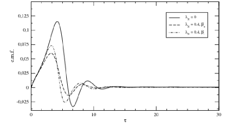
Figure 1: Electromotive force for $\zeta=1$, i.e. strong three-point correlations.

In order to have a simple picture of how ${\bf\varepsilon}_{H}$ evolves, we can reason as follows. For high $R_{M}$ assume a prescribed, negative value for $g^{u}$ in the $\alpha$ term of eq. (20) (i.e, the first term between square brackets), and that the term $\lambda_{H}g^{C}$ is negligible as well as the initial value of $g^{M}$. In that situation $G^{M}$ will initially grow toward positive values (due to the first term of eq. [21]) and $g^{M}$ toward negative values (due to the first term of eq. [22]). This will cause the $\alpha$ term to go to zero at a certain instant, and hence to the end of the kinetic regime, i.e., the period during which the growth of ${\bf B}_{0}$ is exponential. The presence of the $\lambda_{H}g^{C}$ term drastically modifies this scenario: were this term negative, then it would take the $g^{M}$ term a shorter time to cancel the other two terms, i.e., we would have a shorter kinetic phase. Were it positive, then the opposite situation would occur: the kinetic phase would last longer. This simple picture is even more modified by the fact that now the $\beta$ term in eq. (20) (the second term between brackets) is not possitive definite, a fact that could act in favour or against of the two situations described above. We can conclude that the operation of a Hall-MHD dynamo is far more subtle and complicated than the standard MHD one.

4.2 Discussion

To integrate the system we used a 4^th order Runge-Kutta method with variable step and considered the following values for the different parameters that enter in the equations: $r=5$, $g^{u}=-5$ (this value is equivalent to the $g^{u}=-1$ of Blackman & Field fb2002-2 (2002) with the normalization they used), $f^{u}=1$, $R_{M}=2000$ and $\lambda_{H}=0$ and $0.4$. The second value of $\lambda_{H}$ corresponds to a Hall length almost twice the turbulent scale, but shorter than the coherence large scale. The high value of $R_{M}$ is easily found in astrophysical environments. For the three-point correlations we considered two cases: $\zeta=1$ (strong correlations) and $\zeta=2/R_{M}$ (weak correlations). As initial conditions we assumed $Q_{H0}^{\parallel}=0$, $g^{M}_{0}=0.001=G^{M}_{0}$ (i.e., an initial state with small magnetic helicity. Other initial conditions do not give qualitative different results) and $g^{C}=0$. We also considered the two possible signs in the $\beta$ term, namely $\beta_{\pm}=f^{u}\pm\lambda_{H}r|Q_{H}^{\parallel}|$ (see eq. (20)).

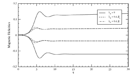
Figure 2: Magnetic helicities for $\zeta=1$, i.e. strong three-point correlations. Upper curves correspond to large scale MH, and lower curves to small scale MH.

In Fig.1 we plotted $Q_{H}^{\parallel}$ as a function of time, for strong nonlinearities, i.e. $\zeta=1$. We see that for $\lambda_{H}\not=0$, $Q_{H}^{\parallel}$ is damped faster than for $\lambda_{H}=0$. For $\beta_{+}$ this process is in turn slightly stronger than for $\beta_{-}$. The saturation value however is the same for all cases, i.e. is not modified by Hall effect. The rise of the first oscilation in the transitory regime corresponds to the kinetic regime, in which the large scale magnetic field would grow exponentially. We see that the instant at which this rise stops is slightly smaller than the one at which stops the standard MHD curve, while the amplitudes of the curves are substantially smaller. This instant is independet of either $\beta_{+}$ or $\beta_{-}$. This behaviour can be interpreted as that the Hall dynamo is less efficient than its standard MHD counterpart to generate large scale fields. In Fig. 2 we plotted small scale magnetic helicity $g^{M}$ (lower curves) and large scale magnetic helicity $G^{M}$ (upper curves), also for $\zeta=1$. We see that for $\lambda_{H}\not=0$ the saturation value of $G^{M}$ is substantially smaller than for $\lambda_{H}=0$, and is the same for both possible $\beta$’s. This means that the inverse cascade of magnetic helicity is suppressed compared to standard MHD, for the considered parameters. Consistently with Fig. 1, we see again that the rise of the first peak takes slightly less time for $\lambda_{H}\not=0$ than for $\lambda_{H}=0$, and the amplitudes in the former case are much smaller than in the latter case.

In Fig. 3 we plotted the e.m.f. $Q_{H0}^{\parallel}$ for $\zeta=2/R_{M}$, i.e. weak non-linearities. The smaller amplitudes of the Hall-MHD curves means that the e.m.f. is more quenched than for standard MHD, as in the case of strong non-linearities. Again in this case the quenching due to $\beta_{+}$ is slightly stronger than the one produced by $\beta_{-}$. In this case the action of Hall effect in the e.m.f. is manifested for all times, as no saturation value is attained. Again here the rise of the first peak corresponds to the kinetic regime, and similar features as for $\zeta=1$ are found: durantion slightly shorter and amplitude significantly smaller, showing that in this case again the Hall-dynamo is less efficient than the standard MHD one. In Fig. 4 we plotted the small scale magnetic helicity $g^{M}$ (lower curves) and the large scale magnetic helicity $G^{M}$ (upper curves). We can appreciate more clearly the quenching produced by Hall effect, as the amplitude of the Hall dynamo is about 5 times shorter than the standard MHD. The comments about the durantion of the kinetic phase are the same as for the $\zeta=1$ case.

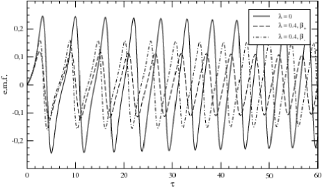
Figure 3: Electromotive force for $\zeta=2/RM$, i.e. weak three-point correlations.

In all figures, the main features (oscillations for the $\zeta=2/R_{M}$ and saturation for $\zeta=1$) are determined by the $\alpha$ term, i.e. by the interplay between kinetic and current small scale helicites, and for the Hall dynamo also by the coupling between small scale magnetic and velocity fields: Given a prescribed negative value of $g^{u}$ in the $\alpha$ term of eq. (20), then $g^{M}$ grows negative, thus leading to a cancellation of them and to a consequent supression of the growth of $Q_{H0}^{\parallel}$ (this is the end of the kinetic regime). In the Hall-dynamo, in the approximation we work with, the $\alpha$ term gets an extra term proportional to $g^{C}$, which in principle can be positive or negative. For the parameters we considered in this work it is negative and consequently reinforces the action of $g^{M}$, thus leading to suppression of the $\alpha$ term faster than in the non-Hall case. Were it positive, then the opposite would occur: it would reinforce $-g^{u}$ and thus it would take longer for the (negative) small scale magnetic helicity to catch up with the other (positive) terms in the $\alpha$ term. As a result the kinetic regime would last longer.

The results quoted in this paper, namely a stronger quenching of the Hall-MHD electromotive force for $\ell_{turbulence}<\ell_{Hall}<\ell_{system}$, agree with numerical simulations performed by Mininni et al (Mininni, Gomez & Mahajan 2003b ).

5 Conclusions

In this paper we studied semianalitically how Hall effect modifies the quenching process of the electromotive force in Mean Field Dynamo theory.We used a dynamical closure scheme named minimal $\tau$ approximation (Blackman & Field fb2002-2 (2002), Brandenburg & Subramanian report-bs (2005)), that takes into account the back-reaction of the small scale fields generated by the turbulence. As we considered helical turbulence, those small scale fields are not to be considered as the result of a small scale dynamo, but as a waste product, that nevertheless strongly quenches the e.m.f.

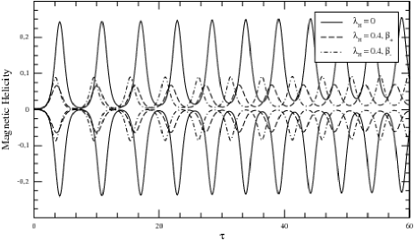
Figure 4: Magnetic helicities for $\zeta=2/RM$, i.e. weak three-point correlations.

Considering force-free large scale magnetic fields, we found that Hall effect modifies the evolution equation of the e.m.f. in several ways: the main driving term, the so-called $\alpha$ term, proportional to $|{\bf B}_{0}|$ now depends on the electronic velocity $u_{e}$ instead of the fluid velocity. Besides there appears a third term, explicitly dependent on the Hall parameter $\ell_{H}$, that couples the magnetic field to this electronic velocity. The diffusive term, also known as $\beta$ term, proportional to $|{\bf\nabla}\times{\bf B}_{0}|$ also depends on the electronic velocity but besides it acquired a new term that couples the small scale magnetic field to the electronic velocity, and that renders it not positive definite. A negative value of this coefficient represents non local transfer from small scale turbulent fields to the large scale magnetic field. Finally there appears a new term proportional to $\nabla^{2}{\bf B}_{0}$. In our case this term plays no significant role because it is substantially smaller than the others due to the perturbative scheme we use.

To give a concrete numerical example, we considered Hall effect as a perturbation of characteristic scale larger than the turbulent scale, but shorter than the large scale magnetic field. This situation can be found in e.g. accretion disks and in the early universe plasma (Sano & Stone stone (2002), Tajima et al. tajima (1992)). After implementing the two scale approximation, we numerically integrated the resulting evolution equations for the e.m.f., the large and small scale magnetic helicities, and the cross-helicity which is the quantity that in this approximation mimics the coupling between the small scale velocity and magnetic fields. The overall effect is that in the presence of Hall effect, the e.m.f. is more strongly quenched than in the case of standard MHD dynamo. This fact is acompanied by a damping in the inverse cascade of magnetic helicity.

As the main scope of this paper is to understand conceptually how Hall effect acts on a MFD, we did not apply our results to a concrete astrophysical object. We leave this issue for future work, after a deeper understanding of the mechanism is attained. Besides this point, this work can be improved in several aspects. A very important one is to extend the perturbative expansion to higher orders (or even to device a non-perturbative scheme) in order to attain other regimes, where dynamo action might be enhanced by Hall effect. This extension might also mean that we should abandon the hypothesis that ${\bf B}_{0}$ is force-free. Next, to work with more general boundary conditions, that permit to relax the conservation of total magnetic helicity. Finally, a more detailed study of the three-point correlations is in order, as well as to consider non-helical turbulence. We are working on some of these topics at present.

Appendix A Evolution Equation for the Electromotive Force

The evolution equation for $\varepsilon_{H}^{\parallel}$ is obtained by calculating

$$\frac{\partial{\bf\varepsilon}_{H}}{\partial t} = \langle\frac{\partial{\bf u}}{\partial t}\times{\bf b}\rangle_{0}+\langle{\bf u}\times\frac{\partial{\bf b}}{\partial t}\rangle_{0}$$ (24)

$$- \ell_{H}\left[\langle\frac{\partial\left({\bf\nabla}\times{\bf b}\right)}{\partial t}\times{\bf b}\rangle_{0}+\langle\left({\bf\nabla}\times{\bf b}\right)\times\frac{\partial{\bf b}}{\partial t}\rangle_{0}\right]\,,$$

and the corresponding equation for ${\bf\varepsilon}_{H}^{\parallel}={\bf\varepsilon}_{H}\cdot\left({\bf B}_{0}/|{\bf B}_{0}|\right)$ by doing ${\partial{\bf\varepsilon}_{H}^{\parallel}}/{\partial t}=\left({\partial{\bf\varepsilon}_{H}}/{\partial t}\right)\left({{\bf B}_{0}}/{|{\bf B}_{0}|}\right)+{\bf\varepsilon}_{H}\left[\partial\left({\bf B}_{0}/|{\bf B}_{0}|\right)/{\partial t}\right]$. Replacing eqs. (8) and (9), considering the development of operator ${\bf\bar{P}}$ to first order in the terms linear in ${\bf B}_{0}$, as is done in Gruzinov & Diamond (gruzinov-2 (1995)), and Blackman & Field (fb2002-2 (2002)), and assuming homogeneous and isotropic turbulence, we obtain:

$$\frac{\partial{\bf\varepsilon}_{H}}{\partial t} = \frac{1}{3}\left\{\langle\left({\bf\nabla}\times{\bf b}\right)\cdot{\bf b}\rangle_{0}-\langle{\bf u}\cdot\left({\bf\nabla}\times{\bf u}\right)\rangle_{0}-\ell_{H}\langle{\bf u}\cdot\nabla^{2}{\bf b}\rangle_{0}\right.$$ (25)

$$+ \ell_{H}\langle{\bf b}\cdot\nabla^{2}{\bf u}\rangle_{0}+\ell_{H}\langle\left({\bf\nabla}\times{\bf b}\right)\cdot\left({\bf\nabla}\times{\bf u}\right)\rangle_{0}$$

$$- \left.\ell_{H}^{2}\langle{\bf b}\cdot\left[{\bf\nabla}\times\nabla^{2}{\bf b}\right]\rangle_{0}+\ell_{H}^{2}\langle\left({\bf\nabla}\times{\bf b}\right)\cdot\nabla^{2}{\bf b}\rangle_{0}\right\}{\bf B}_{0}$$

$$- \frac{1}{3}\left[\langle v^{2}\rangle_{0}+\ell_{H}\langle{\bf\nabla}\cdot\left({\bf u}\times{\bf b}\right)\rangle_{0}\right]\left({\bf\nabla}\times{\bf B}_{0}\right)$$

$$+ \frac{1}{3}\left[\langle{\bf u}\cdot{\bf b}\rangle_{0}-\ell_{H}\langle\left({\bf\nabla}\times{\bf b}\right)\cdot{\bf b}\rangle_{0}\right]\nabla^{2}{\bf B}_{0}$$

$$+ \eta\left[\langle{\bf u}_{e}\times\nabla^{2}{\bf b}\rangle_{0}-\ell_{H}\langle\left({\bf\nabla}\times\nabla^{2}{\bf b}\right)\times{\bf b}\rangle_{0}\right]$$

$$+ \nu\langle\nabla^{2}{\bf u}\times{\bf b}\rangle_{0}+{\bf\bar{T}}\,,$$

where by ${\bf\bar{T}}$ we denote the non linear terms, i.e.:

$${\bf\bar{T}} = \langle{\bf u}\times\left[{\bf\nabla}\times\left({\bf u}\times{\bf b}\right)\right]\rangle_{0}+\langle{\bf\bar{P}}\left(\left[{\bf u}\times\left({\bf\nabla}\times{\bf u}\right)\right]\times{\bf b}\right)\rangle_{0}$$ (26)

$$+ \langle{\bf\bar{P}}\left(\left[\left({\bf\nabla}\times{\bf b}\right)\times{\bf b}\right]\times{\bf b}\right)\rangle_{0}-\ell_{H}\langle{\bf u}\times\left\{{\bf\nabla}\times\left[\left({\bf\nabla}\times{\bf b}\right)\times{\bf b}\right]\right\}\rangle_{0}$$

$$- \ell_{H}\langle\left({\bf\nabla}\times{\bf b}\right)\times\left[{\bf\nabla}\times\left({\bf u}\times{\bf b}\right)\right]\rangle_{0}-\ell_{H}\langle\left\{{\bf\nabla}\times\left[{\bf\nabla}\times\left({\bf u}\times{\bf b}\right)\right]\right\}\times{\bf b}\rangle_{0}$$

$$+ \ell_{H}^{2}\langle\left({\bf\nabla}\times{\bf b}\right)\times\left\{{\bf\nabla}\times\left[\left({\bf\nabla}\times{\bf b}\right)\times{\bf b}\right]\right\}\rangle_{0}$$

$$+ \ell_{H}^{2}\langle\left[{\bf\nabla}\times\left\{{\bf\nabla}\times\left[\left({\bf\nabla}\times{\bf b}\right)\times{\bf b}\right]\right\}\right]\times{\bf b}\rangle_{0}\,.$$

Recalling that ${\bf u}_{e}={\bf u}-\ell_{H}{\bf\nabla}\times{\bf b}$, we can write eq. (25) in a form that shows explicitly that now it is the electronic flow the driver of the dynamo:

$$\frac{\partial{\bf\varepsilon}_{H}}{\partial t} = \frac{1}{3}\left\{\langle\left({\bf\nabla}\times{\bf b}\right)\cdot{\bf b}\rangle_{0}-\langle{\bf u}_{e}\cdot\left({\bf\nabla}\times{\bf u}_{e}\right)\rangle_{0}+\ell_{H}\langle{\bf b}\cdot\nabla^{2}{\bf u}_{e}\rangle_{0}\right\}{\bf B}_{0}$$ (27)

$$- \frac{1}{3}\left[\langle{\bf u}\cdot{\bf u}_{e}\rangle_{0}+\ell_{H}\langle{\bf b}\cdot\left({\bf\nabla}\times{\bf u}\right)\rangle_{0}\right]\left({\bf\nabla}\times{\bf B}_{0}\right)$$

$$+ \frac{1}{3}\langle{\bf u}_{e}\cdot{\bf b}\rangle_{0}\nabla^{2}{\bf B}_{0}+\eta\left[\langle{\bf u}_{e}\times\nabla^{2}{\bf b}\rangle_{0}-\ell_{H}\langle\left({\bf\nabla}\times\nabla^{2}{\bf b}\right)\times{\bf b}\rangle_{0}\right]$$

$$+ \nu\langle\nabla^{2}{\bf u}\times{\bf b}\rangle_{0}+{\bf\bar{T}}\,.$$