Refined parameters of the planet orbiting HD 189733

Abstract

We report on the BVRI multi-band follow-up photometry of the transiting extrasolar planet HD 189733b. We revise the transit parameters and find planetary radius $R_{\rm P}=1.154\pm 0.032R_{\rm J}$ and inclination $i_{\rm P}=85.79\pm 0.24\arcdeg$. The new density ($\rm\sim 1g\,cm^{-3}$) is significantly higher than the former estimate ($\rm\sim 0.75g\,cm^{-3}$); this shows that from the current sample of 9 transiting planets, only HD 209458 (and possibly OGLE-10b) have anomalously large radii and low densities. We note that due to the proximity of the parent star, HD 189733b currently has one of the most precise radius determinations among extrasolar planets. We calculate new ephemerides: $P=2.218573\pm 0.000020$ days, $T_{0}=2453629.39420\pm 0.00024$ (HJD), and estimate the timing offsets of the 11 distinct transits with respect to the predictions of a constant orbital period, which can be used to reveal the presence of additional planets in the system.

1. Introduction

HD 189733 is one of nine currently known main sequence stars orbited by a transiting giant planet. The system is of exceptional interest because it is the closest known transiting planet (D = 19.3pc), and thus is amenable to a host of follow-up observations. The discovery paper by Bouchy et al. (2005) (hereafter B05) derived the key physical characteristics of the planet, namely its mass ($1.15\pm 0.04M_{\rm J}$) and radius ($1.26\pm 0.03R_{\rm J}$), based on radial velocity observations of the star made with the ELODIE spectrograph at the 1.93m telescope at Observatoire de Haute Provence (OHP), together with photometric measurements of one complete and two partial transits made with the 1.2m telescope also at OHP. With these parameters HD 189733b had a large radius comparable to HD 209458b (Laughlin et al., 2005), and a density roughly equal to that of Saturn ($\rho\sim 0.7\rm g\,cm^{-3}$).

Determining precise radii of extrasolar planets in addition to their mass is an important focus of exoplanet research (see e.g. Bouchy et al., 2004; Torres et al., 2004), because the mean density of the planets can shed light on their internal structure and evolution. According to Baraffe et al. (2005), the radii of all known extrasolar planets are broadly consistent with models, except for HD 209458b. This planet with its large radius and low density ($\rho\sim 0.33\rm g\,cm^{-3}$) has attracted considerable interest, and various mechanisms involving heat deposition beneath the surface have been suggested (Laughlin et al., 2005, and references therein). An additional motivation for obtaining accurate planetary radii is proper interpretation of follow-up data, notably secondary eclipse and reflected light observations. This is of particular relevance to HD 189733b, which has been recently observed by the Spitzer Space Telescope (Deming et al., 2006), and where the brightness temperature depends on the radius ratio of the planet to the star.

Both by extending the current, very limited sample of transiting exoplanets, and by precise determination of the physical parameters it will become possible to refine theoretical models and decide which planets are “typical”. Close-by, bright stars, such as the host star of HD 189733 are essential in this undertaking. The OGLE project (Udalski et al., 2002a, b, c) and follow-up observations (e.g. Konacki et al., 2004; Moutou et al., 2004; Pont et al., 2005) made a pivotal contribution to the current sample by the discovery of more than half of the known transiting planets. Follow-up observations, however, are cumbersome due to the faintness of the targets, and required the largest available telescopes. The typical errors of mass and radius for these host stars are $\sim 0.06M_{\sun}$ and $\sim 0.15R_{\sun}$, and the corresponding errors in planetary parameters are $\sim 0.13M_{\rm J}$ and $\sim 0.12R_{\rm J}$, respectively. However, for planets orbiting bright stars in the solar neighborhood, errors at the level of a few percent can be reached for both the mass and radius.

In this paper we report a number of follow-up photometric measurements of HD 189733 using six telescopes spaced around the world. Together with the original OHP photometry, we use these measurements to determine revised values for the transit parameters, and give new ephemerides. First we describe the follow-on photometry in detail (§2), followed by the modeling which leads to the revised estimate of the planetary radius (§3), and we conclude the paper in §4.

Table 1 Summary of instruments used in the observing campaign of HD 189733.

Site	Longitude	Latitude	Alt.	Telescope	Diam.	Detector	Pxs	$T_{rd}$	FOV
			(meters)		(meters)		($\rm\arcsec/pix$)	(sec)
OHP	05°30′ E	43°55′ N	650	OHP1.2	1.2	SITe $\rm 1K\times\rm 1K$	0.69	90	11.77′
FLWO	110°53′ W	31°41′ N	2350	FLWO1.2	1.2	Fairchild $\rm 4K\times\rm 4K$	0.34	12	23′
FLWO	110°53′ W	31°41′ N	2345	HAT-5	0.11	Thomson $\rm 2K\times\rm 2K$	14.0	10	8.2°
FLWO	110°53′ W	31°41′ N	2345	HAT-6	0.11	Thomson $\rm 2K\times\rm 2K$	14.0	10	8.2°
FLWO	110°53′ W	31°41′ N	2345	TopHAT	0.26	Marconi $\rm 2K\times\rm 2K$	2.2	40	1.29°
Mauna Kea	155°28′ W	19°49′ N	4163	HAT-9	0.11	Thomson $\rm 2K\times\rm 2K$	14.0	10	8.2°
Wise	34°35′ E	30°35′ N	875	Wise1.0	1.0	Tektronics $\rm 1K\times\rm 1K$	0.7	40	11.88′

2. Observations and Data Reduction

We organized an extensive observing campaign with the goal of acquiring multi-band photometric measurements of the transits of HD 189733 caused by the hot Jupiter companion. Including the discovery data of B05 that were obtained at OHP, altogether four sites with seven telescopes contributed data to two full and eight partial transits in Johnson B, V, R, I and Sloan r photometric bandpasses. The sites and telescopes employed are spread in geographic longitude, which facilitated gathering the large number (close to 3000) of individual data spanning 2 months.

The following telescopes were involved in the photometric monitoring: the 1m telescope at the Wise Observatory, Israel; the 1.2m telescope at OHP; the 1.2m telescope at Fred Lawrence Whipple Observatory (FLWO) of the Smithsonian Astrophysical Observatory (SAO); the 0.11m HAT-5 and HAT-6 wide field telescopes plus the 0.26m TopHAT telescope also at FLWO; and the 0.11m HAT-9 telescope at the Submillimeter Array site at Mauna Kea, Hawaii. An overview of the sites and telescopes is shown in Table 1.

A summary of the observations is shown in Table 2. The telescopes are identified by the same names as in Table 1. The transits have been numbered starting with the discovery data $N_{tr}\equiv 0$, and are identified later in the text using this number. In the following subsections we summarize the observations and reductions that are specific to the sites or instruments.

Table 2 Summary of HD 189733 observations.

Telescope	Filter	$N_{tr}$	Epoch	Date	Transit	Cond.	$\sigma_{OOT}$	$\sigma_{sys}$	Cad.	Ap[″]
				(UT)			(mmag)	(mmag)	(sec)	(″)
OHP1.2	B	0	53629.4	2005-09-15	OIBEO	5	2.6	1.3	86	10
Wise1.0	B	4	53638.3	2005-09-24	-IBE-	4	$\cdots$	$\cdots$	42	5
OHP1.2	$\rm R_{c}$	4	53638.3	2005-09-24	--BEO	4	3.0	1.2	95	10
OHP1.2	$\rm R_{c}$	5	53640.5	2005-09-26	OI---	3	6.8	2.4	95	10
FLWO1.2	r	6	53642.7	2005-09-29	OIBEO	4	2.6	0.5	17	20
HAT-5	$\rm I_{c}$	6	53642.7	2005-09-29	OIBEO	4	4.4	1.3	135	42
HAT-6	$\rm I_{c}$	6	53642.7	2005-09-29	OIBEO	4	4.1	1.2	108	42
TopHAT	V	6	53642.7	2005-09-29	OIBEO	4	4.6	3.0	70	10
HAT-9	$\rm I_{c}$	7	53644.9	2005-10-01	OIB--	4	4.6	1.2	99	42
HAT-9	$\rm I_{c}$	16	53664.9	2005-10-21	OIB--	4	4.3	$\cdots$	100	42
TopHAT	V	19	53671.6	2005-10-28	---eO	4	5.3	$\cdots$	106	10
HAT-5	$\rm I_{c}$	19	53671.6	2005-10-28	---EO	4	4.6	$\cdots$	103	42
HAT-5	$\rm I_{c}$	20	53673.8	2005-10-30	OIb--	5	3.3	0.9	85	42
Wise1.0	B	22	53678.2	2005-11-03	--bEO	3	5.5	1.1	49	10
TopHAT	V	24	53682.6	2005-11-08	OIb--	2	5.4	2.6	108	10
HAT-9	$\rm I_{c}$	29	53693.7	2005-11-19	-IBEO	5	6.6	1.1	90	42

Note. — The table summarizes all observations that were part of the observing campaign described in this paper. Not all of them were used for refining the ephemerides or parameters of the transit – see Table 3 and Table 5 for reference. $\mathbf{N_{tr}}$ shows the number of transits since the discovery data. Epoch and Date show the approximate time of mid-transit. The Transit column describes in a terse format which parts of the transits were observed; Out-of-Transit (OOT) section before the transit, Ingress, Bottom, Egress and OOT after the transit. Missing sections are indicated by ”–”. The Conditions column indicates the photometric conditions on the scale of 1 to 5, where 5 is absolute photometric, 4 is photometric most of the time with occasional cirrus/fog (relative photometric), 3 stands for broken cirrus, and 2 for poor conditions. Column $\sigma_{OOT}$ gives the rms of the OOT section at the Cadence shown in the next column. If the transit was full, $\sigma_{OOT}$ was computed separately from the pre- and post-transit data, and the smaller value is shown. Column $\sigma_{sys}$ shows the estimated amplitude of systematics (for details, see §3.2). Ap shows the aperture used in the photometry in arcseconds.

2.1. Observations by OHP 1.2m telescope

These observations and their reduction were already described in B05. Summarizing briefly, the 1.20m f/6 telescope was used together with a $\rm 1K\times\rm 1K$ back-illuminated CCD having 0.69$\rm\arcsec/pix$ resolution. Typical exposure times were 6 seconds long, followed by a 90 second readout. The images were slightly defocused, with FWHM$\approx$2.8″.

Full-transit data were obtained in Johnson B-band under photometric conditions for the $N_{tr}=0$ transit. This is shown by the “OIBEO” flag in Table 2 indicating that the Out-of-transit part before the Ingress, the Bottom, the Egress, and the Out-of-transit part after egress all have been observed. This is an important part of the combined dataset, as it is the only full transit seen in B-band. In addition, partial transit data were obtained for the $N_{tr}=4$ event using Cousin’s R-band filter ($R_{C}$) under acceptable photometric conditions, and for the $N_{tr}=5$ event using the same filter under non-photometric conditions. The frames were subject to bias, dark and flatfield calibration procedure followed by cosmic ray removal. Aperture photometry was performed in an aperture of 9.6″ using the daophot (Stetson, 1987) package.

The B-band light-curve published in the B05 discovery paper used the single comparison star HD 345459. This light-curve suffered from a strong residual trend, as suggested by the $\sim 0.01mag$ difference between the pre- and post-transit sections. This trend was probably a consequence of differential atmospheric extinction, and was removed by a linear airmass correction, bringing the two sections to the same mean value. This ad-hoc correction, however, may have introduced an error in the transit depth. In this paper, we used six comparison stars in the field of view (selected to have comparable relative flux to HD 189733 before and after transit). A reference light-curve was built by co-adding the normalized flux of all six stars, and was subtracted from the normalized light-curve of HD 189733. The new reduction shows a residual OOT slope 4.2 times smaller than in the earlier reduction. The resulting transit depth in B-band is decreased by about 20% compared to the discovery data. This illustrates the large contribution of photometric systematics that must be accounted for in this kind of measurement. The R-band data set is not as sensitive to the extinction effect as the B-band, hence the selection of comparison stars has a minimal impact on the shape of the transit curve. The B-band light-curve is shown on panel 6 of Fig. 1, the R-band light-curves are exhibited in Fig. 2.

2.2. Observations by the FLWO 1.2m telescope

We used the FLWO 1.2m telescope to observe the full transit of $N_{tr}=6$ in Sloan r band. The detector was Keplercam , which is a single chip $\rm 4K\times\rm 4K$ CCD with 15µm pixels that correspond to 0.34″ on the sky. The entire field-of-view is 23′. The chip is read out by 4 amplifiers, yielding a 12 second readout with the $2\times 2$ binning we used. The single-chip design, wide field-of-view, high sensitivity and fast readout make this instrument well-suited for high-quality photometry follow-up.

The target was deliberately defocused in order to allow longer exposure times without saturating the pixels, and to smear out the inter-pixel variations that may remain after flatfield calibration. The intrinsic FWHM was $\sim 2\arcsec$, which was defocused to $\sim 10\arcsec$. While conditions during the transit were photometric, there were partial clouds before and after. The focus setting was changed twice during the night; first when the clouds cleared, and second, when the seeing improved. In both cases the reason was to keep the signal level within the linear response range of the CCD. We used a large enough aperture that these focus changes did not affect the photometry. All exposures were 5 seconds in length with 12 seconds of readout and overhead time between exposures. We observed the target in a single band so as to maximize the cadence, and to eliminate flatfielding errors that may originate from the imperfect sub-pixel re-positioning of the filter-wheel. Auto-guiding was used to further minimize systematic errors that originate from the star drifting away on the CCD chip and falling on pixels with different (and not perfectly calibrated) characteristics.

Reduction and photometry

All images were reduced in the same manner; applying overscan correction, subtraction of the two-dimensional residual bias pattern and correction for shutter effects. Finally we flattened each image using a combined and normalized set of twilight sky flat images. There was a drift of only $\sim 3\arcsec$ in pointing during the night, so any large-scale flatfielding errors were negligible.

To produce a transit light curve, we chose one image as an astrometric reference and identified star centers for HD 189733 and 23 other bright and relatively uncrowded stars in the field. We measured the flux of each star around a fixed pixel center derived from an astrometric fit to the reference stars, in a 20$\arcsec$ circular aperture using daophot/phot within iraf (Tody, 1986, 1993) and estimated the sky using the sigma-rejected mode in an annulus defined around each star with inner and outer radii of 33$\arcsec$ and 60$\arcsec$ respectively.

We calculated the extinction correction based on a weighted mean flux of comparison stars and applied this correction to each of our stars. We iteratively selected our comparison stars by removing any that showed unusually noisy or variable trends in their differential light curves. Additionally, a few exposures in the beginning and very end of our observing sequence were removed because those observations were made through particularly thick clouds. The resulting light curve represents the observed counts for the star corrected for extinction using a group of 6 comparison stars within 6$\arcmin$ separation from HD 189733. The light-curve is shown on panels 3 and 4 of Fig. 1.

2.3. Observations by HATNet

An instrument description of the wide-field HAT telescopes was given in Bakos et al. (2002, 2004). Here we briefly recall the relevant system parameters. A HAT instrument contains a fast focal ratio (f/1.8) 0.11m diameter Canon lens and Peltier-cooled CCD with a front-illuminated $\rm 2K\times\rm 2K$ chip having 14µm pixel size. The resulting FOV is 8.2° with 14″ pixel scale. Using a psf-broadening technique (Bakos et al., 2004), careful calibration procedure, and robust differential photometry, the HAT telescopes can achieve 3mmag precision (rms) light-curves at 300s resolution for bright stars (at $I\approx 8$). The HAT instruments are operated in autonomous mode, and carry out robotic observations every clear night.

We have set up a longitude-separated, two-site network of six HAT instruments, with the primary goal being detection of planetary transits in front of bright stars. The two sites are FLWO, in Arizona, the same site where the 1.2m telescope is located (§2.2), and the roof of the Submillimeter Array atop Mauna Kea, Hawaii (MK).

In addition to the wide-field HAT instruments, we developed a dedicated photometry follow-up instrument, called TopHAT, which is installed at FLWO. A brief system description was given in Charbonneau et al. (2006) in context of the photometry follow-up of the HD 149026 planetary transit. This telescope is 0.26m diameter, f/5 Ritchey-Crétien design with a Baker wide-field corrector. The CCD is a $\rm 2K\times\rm 2K$ Marconi chip with 13.5µm pixel size. The resulting FOV is 1.3° with 2.2″ pixel resolution. Similarly to the HATs, TopHAT is fully automated.

Selected stations of the HAT Network, along with TopHAT, observed one full and six partial transits of HD 189733 (for details, see Table 2). Observing conditions of the full-transit event at FLWO at $N_{tr}=6$ have been summarized in §2.2. This transit was observed by HAT-5 and HAT-6 (both in I-band), and by TopHAT (V-band). The partial transit observations at numerous later epochs included HAT-5 (FLWO, I-band), HAT-9 (MK, I-band) and TopHAT (FLWO, V-band). Typical exposure times for the wide-field instruments were 60 to 90 seconds with 10 second readout. TopHAT exposures were $\sim$12sec long with up to 40 second readout and download time. All observations were made at slight defocusing and using the psf-broadening technique. The stellar profiles were 2.5pix (35″) and 4.5pix (9.9″) wide for the HATs and TopHAT, respectively. Although we have no auto-guiding, real-time astrometry was performed after the exposures, and the telescope’s position was kept constant with 20″ accuracy.

Reduction and photometry

All HAT and TopHAT images were subject to overscan correction, two-dimensional residual bias pattern and dark subtraction, and normalization with a master sky-flat frame. Bias, dark and sky-flat calibration frames were taken each night by each telescope, and all object frames were corrected with the master calibration images that belonged to the specific observing session. Saturated pixels were masked before the calibration procedure.

We used the 2MASS All-Sky Catalog of Point Sources (Skrutskie et al., 2000; Cutri et al., 2003) as an input astrometric catalogue, where the quoted precision is 120 mas for bright sources. A 4th order polynomial fit was used to transform the 2MASS positions to the reference frame of the individual images. Typical rms of the transformations was 700 mas for the wide-field instruments, and 150 mas for TopHAT.

Fixed center aperture photometry was performed for all these stars. For the wide-field HAT telescopes we used an $r_{ap}=3$ pixel (42″) aperture, surrounded by an annulus with inner and outer radii of $r_{1}=5$ pix (70″) and $r_{2}=13$ pix (3′), respectively. For TopHAT, the best aperture was $r_{ap}=5$ pix (10.8″) with $r_{1}=13$ pix (29″) and $r_{2}=21$ pix (46″). The apertures were small enough to exclude any bright neighboring star.

A high quality reference frame was selected for the wide-field HAT telescopes from the Mauna Kea HAT-9 data, and separately for TopHAT. Because the HAT wide field instruments are almost identical, we were able to use the HAT-9 reference frame to transform the instrumental magnitudes of HAT-5 and HAT-6 data to a common system. For this, we used 4th order polynomials of the magnitude differences as a function of X and Y pixel positions. In effect, we thereby used $\sim 3000$ and $\sim 800$ selected non-variable comparison stars for the HATs, and TopHAT, respectively. This contributes to the achieved precision, which is only slightly inferior to the precision achieved by the bigger diameter telescopes.

The amount of magnitude correction for HD 189733 between the reference and the individual images is shown in the $\Delta M_{ext}$ column of Table 3. The same table also indicates the rms of these magnitude fits in the $\sigma_{mfit}$ column. Both quantities are useful for further cleaning of the data. Because HD 189733 is a bright source, it was saturated on a small fraction of the frames. Saturated data-points were flagged in the light-curves, and also de-selected from the subsequent analysis (flagged as “C” in Table 3).

After cleaning outliers by automatically de-selecting points where the rms of the magnitude transformations was above a critical threshold (typically 25mmag) the light-curves reached a precision of $\sim$4mmag at 90 second resolution for both the HATs and TopHAT. Full-transit data are shown in panels 1, 2 and 5 of Fig. 1, and partial-transit data are shown in Fig. 2.

2.4. Observations by the Wise 1.0m telescope

The Wise 1m f/7 telescope was used to observe the $N_{tr}=4$ and $N_{tr}=22$ transits in B-band. The CCD was a $\rm 1K\times\rm 1K$ Tektronics chip with 24µm pixel size that corresponds to 0.696$\rm\arcsec/pix$ resolution on the sky, and a FOV of 11.88′. The photometric conditions were acceptable on both nights, with FWHM$\approx$2″. Auto-guiding was used during the observations. Frames were calibrated in a similar manner to the FLWO1.2m observations, using twilight flats, and aperture photometry was performed with daophot.

Unfortunately, out-of-transit (OOT) data of the first transit ($N_{tr}=4$) (which was also observed from OHP in R-band) are missing, so it is impossible to obtain useful normalization or to apply extinction correction to the transit curve. The second transit ($N_{tr}=22$) was processed using an aperture of 10″ encircled by an annulus with inner and outer radii of 15″ and 25″, respectively. Seven comparison stars were used, all of them bright, isolated and far from the boundary of the FOV. Extinction correction, derived from the OOT points only, was applied to the resulting stellar light-curve. The final curve of this transit is plotted in Fig. 2.

2.5. The resulting light-curve

All photometry originating from the individual telescopes which contains significant OOT data has been merged, and is presented in Table 3. We give both the ratio of the observed flux to the OOT flux of HD 189733 (“FR”), and magnitudes that are very close to the standard Johnson/Cousins system (“Mag”). Due to the different observing conditions, instruments, photometry parameters (primarily the aperture) and various systematic effects (changing FWHM), the zero-point of the observations were slightly offset. Even for the same instrument, filter-setup, and magnitude reference frame, the zero-points in the flat OOT section were seen to differ by $0.03$mag. The offset can be explained by long-term systematic variations and by intrinsic variation of HD 189733.

In order to correct for the offsets, for each transit observation (as indicated by $N_{tr}$ in Table 3) we calculated both the median value from the OOT section by rejecting outliers, and also the rms around the median. The OOT median was used for two purposes. First, we normalized the flux values of the given light-curve segment at $N_{tr}$, which are shown in the “FR” (flux-ratio) column of Table 3. Second, we shifted the magnitudes to the standard system in order to present reasonable values in the “Mag” column. For the standard system we used the Hipparcos values, except for R-band, which was derived by assuming $R-I=0.48$ from Cox (2000).

The formal magnitude errors that are given in the “Merr” column are based on the photon-noise of the source and the background-noise (e.g.  Newberry, 1991). They are in a self-consistent system, but they underestimate the real errors, which have contributions from other noise factors, such as i) scintillation (Young, 1967; Gilliland & Brown, 1988), ii) calibration frames (Newberry, 1991), iii) magnitude transformations depending on the reference stars and imperfectly corrected extinction (indicators of this error source are the $\Delta M_{ext}$ extinction and the $\sigma_{mfit}$ rms of extinction corrections in Table 3). Because it is rather difficult to calculate these factors, we assumed that the observed rms in the OOT section of the light-curves is a relevant measure of the overall noise, and used this to normalize the error estimates of the individual flux-ratios (column “FRerr”, see later §2.6).

Table 3 The light-curve of HD 189733.

Tel.	Fil.	$N_{tr}$	HJD	Mag	Merr	FR	$\rm FR_{corr}$	$\rm FR_{err}$	$\Delta M_{ext}$	$\sigma_{mfit}$	Qflag
					(mag)				(mag)	(mag)
OHP1.2	B	0	2453629.3205430	8.6062	$\cdots$	0.99614	0.99612	$\cdots$	$\cdots$	$\cdots$	$\cdots$
FLWO1.2	r	6	2453642.6001600	7.1886	0.0008	1.02934	1.02972	0.00074	$\cdots$	$\cdots$	$\cdots$
HAT-5	I	6	2453642.5903353	6.7452	0.0017	0.99522	0.99511	0.00156	-0.147	0.0142	G
HAT-6	I	6	2453642.6082715	6.7357	0.0017	1.00397	1.00406	0.00156	-0.011	0.0160	G
TopHAT	V	6	2453642.6042285	7.6717	0.0009	0.99844	0.99841	0.00083	-0.097	0.0080	G
HAT-9	I	7	2453644.8307479	6.7383	0.0019	1.00157	1.00160	0.00175	-0.015	0.0081	G
Wise1.0	B	22	2453678.1963150	8.6374	0.0013	0.96792	0.96779	0.00120	$\cdots$	$\cdots$	$\cdots$

Note. — This table is published in its entirety (2938 lines) in the electronic edition of the paper. A portion is shown here regarding its form and content with a sample line for each telescope in the order they observed a transit with an OOT section. Column $\mathbf{N_{tr}}$ is the number of transits since the discovery data by OHP on $\rm HJD=2453629.3$. Values in the Mag (magnitude) column have been derived by shifting the zero-point of the particular dataset at $N_{tr}$ to bring the median of the OOT section to the standard magnitude value in the literature. Merr (and $\rm FR_{err}$) denote the formal magnitude (and flux-ratio) error estimates based on the photon and background noise (not available for all data). The flux-ratio $\bf FR$ shows the ratio of the individual flux measurements to the sigma-clipped median value of the OOT at that particular $N_{tr}$ transit observation. The merger-corrected flux-ratio $\rm FR_{corr}$ is described in detail in §2.6. The $\mathbf{\Delta M_{ext}}$ is a measure of the extinction on a relative scale (instrumental magnitude of reference minus image), $\mathbf{\sigma_{mfit}}$ is the rms of the magnitude fit between the reference and the given frame. Both of these quantities are useful measures of the photometric conditions. Qflag is the quality flag: “G” means good, “C” indicates that the measurement should be used with caution, e.g. the star was marked as saturated. Fit of the transit parameters were performed using the HJD, FR, $\rm FR_{corr}$ and $\rm FR_{err}$ columns.

2.6. Merger analysis

HD 189733 has a number of faint, close-by neighbors that can distort the light-curve, and may bias the derived physical parameters. These blends can have the following second-order effects: i) the measured transit will appear shallower, as if the planetary radius was smaller, ii) the depth and shape of the transit will be color-dependent in a different way than one would expect from limb-darkening models, iii) differential extinction can yield an asymmetric light-curve, iv) variability of a faint blend can influence the observed light-curve. Our goal was to calculate the additional flux in the various apertures and bandpasses shown in Table 2, and correct our observed flux-ratios (Table 3, column FR) to a realistic flux-ratio ($\rm FR_{corr}$).

The 2MASS point-source catalogue (Cutri et al., 2003) lists some 30 stars within 45″, which is the aperture used at the HAT-5,6,9 telescopes, 5 stars within 20″ (FLWO1.2m), and 3 stars within 15″, which may affect the measurements of the 10″ apertures of OHP1.2, Wise1.0 and TopHAT (apertures are listed in Table 2). To check the reality of listed blends, and to search for additional merger stars, we inspected the following sources: the Palomar Observatory Sky Survey (POSS I) red plates (epoch 1951), the Palomar Quick-V Survey (QuickV, epoch 1982), the Second Palomar Sky Survey (POSS II) plates (epoch 1990 – 1996), the 2MASS J, H and $K_{S}$ scans (epoch 2000), and our own images. We can use the fact that HD 189733 is a high proper motion star with velocity of $\sim 0.25\arcsec/yr$ pointing South. It was $\sim 13\arcsec$ to the North on the POSS-I plates, and $\sim 4\arcsec$ N on POSS-II, thus we can check its present place when it was not hidden by the glare of HD 189733. The analysis is complicated by the saturation, diffraction spikes, and the limited scan resolution (1.7$\rm\arcsec/pix$) of POSS-I, but we can confirm that there is no significant source at the epoch 2005 position of HD 189733 down to $\sim$4mag fainter in R-band. The reality of all the 2MASS entries was double checked on the POSS frames.

There are only two additional faint sources that are missing from the 2MASS point-source catalogue, but detected by our star-extraction on the 2MASS J, H and K scans; the first one at $\alpha=20^{h}00^{m}45.12^{s}$, $\delta=+22\arcdeg 42\arcmin 36.5\arcsec$ and the second at $\alpha=20^{h}00^{m}43.20^{s}$, $\delta=+22\arcdeg 42\arcmin 42.5\arcsec$. We made sure these sources are not filter-glints or persistence effects on the 2MASS scans; they are also visible on the POSS frames. Their instrumental magnitude was transformed to the J,H,$K_{S}$ system using the other stars in the field that are identified in the point source catalogue.

A rough linear transformation was derived between the 2MASS J, H and $K_{S}$ colors and Johnson/Cousins B, V, R and I by cross-identification of $\sim 450$ Landolt (1992) standard stars, and performing linear regression. The uncertainty in the transformation can be as large as 0.1mag, but this is adequate for the purpose of estimating the extra flux (in BVRI), which is only about a few percent that of HD 189733.

We find that the extra flux in a 45″  aperture is $\delta=$ 1.012, 1.016, 1.018 and 1.022 times the flux of HD 189733 in B, V, R and I-bands, respectively. The dominant contribution comes from the red star 2MASS 20004297+2242342 at 11.5″ distance, which is $\sim$4.5mag fainter. This star has been found (Bakos et al., 2006) to be a physical companion to HD 189733 and thus may also be called HD 189733B (not to be confused with HD 189733b). For the 10″ aperture we assumed that half the flux of HD 189733B is within the aperture. The same $\delta$ flux contribution in the 10″ aperture is 1.003, 1.005, 1.006 and 1.008 in BVRI. The corrected flux-ratios of the individual measurements to the median of the OOT were calculated in the manner $\rm FR_{corr}=1+\delta\cdot(FR-1)$, and are shown in Table 3. There is a small difference ($\sim$2%) between the 10″ and 45″ flux contribution, thus we expect that the former measurements (OHP1.2, Wise1.0, TopHAT) show slightly deeper transits than the FLWO1.2m (r) and wide-field HATNet telescopes (I).

3. Deriving the physical parameters of the system

We use the full analytic formula for nonlinear limb-darkening given in Mandel and Agol (2002) to calculate our transit curves. In addition to the orbital period and limb-darkening coefficients, these curves are a function of four variables, including the mass ($M_{*}$) and radius ($R_{*}$) of the star, the radius of the planet ($R_{\rm P}$), and the inclination of the planet’s orbit relative to the observer ($i_{\rm P}$). Because these parameters are degenerate in the transit curve, we use $M_{*}=0.82\pm 0.03M_{\sun}$ from B05 to break the degeneracy. As regards $R_{*}$, there are two possible approaches: i) assume a fixed value from independent measurements (§3.1), ii) measure the radius of the star directly from the transit curve, i.e. leave it to vary freely in the fit. Our final results are based on detailed analysis (§3.2) using the first approach. To fully trust the second approach, one would need high precision data with relatively small systematic errors. Nevertheless, in order to check consistency, we also performed an analysis where the stellar radius was left as a variable in the fit, and also checked the effect of systematic variations in the light-curves (see later in §3.2). Refined ephemerides and center of transit time residuals are discussed in §3.3.

3.1. The radius of HD 189733

Because the value of the stellar radius we use in our fit linearly affects the size of the planet radius we obtain, we use several independent methods to check its value and uncertainty.

First method

For our first calculation we use 2MASS (Cutri et al., 2003) and Hipparcos photometry (Perryman et al., 1997) to find the V-band magnitude and V-K colors of the star, and use the relation described in Kervella et al. (2004) to find the angular size of the star. Because this relation was derived using Johnson magnitudes, we first convert the 2MASS $\rm K_{S}=5.541\pm 0.021$ magnitude to the Bessell-Brett homogenized system, which in turn is based on the SAAO system, and thus is the closest to Johnson magnitude available (Carpenter, 2005). We obtain a value of $K=5.59\pm 0.05$. Most of the error comes from the uncertainty in the $\rm J-\rm K_{S}$ color, which is used in the conversion.

The Johnson V-band magnitude from Hipparcos is $7.67\pm 0.01$. This gives a V-K color of $2.09\pm 0.06$. From Kervella et al. (2004), the limb-darkened angular size of a dwarf star is related to its K magnitude and V-K color by:

$$log(\theta)=0.0755(V-K)+0.5170-0.2K\,.$$ (1)

Given the proximity of HD 189733 ($19.3\pm 0.3$pc), reddening can be neglected, despite its low galactic latitude. The relation gives an angular size of $0.36\pm 0.02$mas for the stellar photosphere, where the error estimate originates from the errors of V-K and K. The small dispersion of the relation was not taken into account in the error estimate, as it was determined by Kervella et al. (2004) using a fit to a sample of stars with known angular diameters to be less than 1%. Using the Hipparcos parallax we find that $R_{*}=0.75\pm 0.05R_{\sun}$.

Second method

We also derive the radius of the star directly from the Hipparcos parallax, V-band magnitude, and temperature of the star. We first convert from apparent magnitude to absolute magnitude and apply a bolometric correction (Bessell et al., 1998). To solve for the radius of the star we use the relation:

$$M_{b}=4.74-2.5log\left[\left(\frac{T_{eff,*}}{T_{eff,\sun}}\right)^{4}\left(\frac{R_{*}}{R_{\sun}}\right)^{2}\right]$$ (2)

For $T_{eff,*}=5050\pm 50$ K effective temperature (B05), we measure a radius of $0.74\pm 0.03R_{\sun}$.

Third method – isochrones

An additional test on the stellar radius and its uncertainty comes from stellar evolution models. We find from the Girardi et al. (2002) models that the isochrone gridpoints in the ($T_{\rm eff}$, $\log{g}$) plane that are closest to the observed values ($T_{eff,*}=5050\pm 50K$, $\log{g}=4.53\pm 0.14$) prefer slightly evolved models with $M_{*}\approx 0.80M_{\sun}$ and $R_{*}\approx 0.79R_{\sun}$. Alternatively, the Hipparcos $V=7.67\pm 0.01$ magnitude, combined with the $m-M=-1.423\pm 0.035$ distance modulus yields $M_{V}=6.25\pm 0.04$ absolute V magnitude, and the closest isochrone gridpoints prefer less evolved stars with $M_{*}\approx 0.80M_{\sun}$ and $R_{*}\approx 0.76R_{\sun}$. The discrepancy between the above two approaches decreases if we adopt a slightly larger distance modulus. Finally, comparison to the Baraffe et al. (1998) isochrones yields $M_{*}\approx 0.80M_{\sun}$ and $R_{*}\approx 0.76R_{\sun}$. From isochrone fitting, the error on the stellar radius can be as large as 0.03$R_{\sun}$.

Fourth method

Recently Masana et al. (2006) calibrated the effective temperatures, angular semi-diameters and bolometric corrections for F, G, K type stars based on V and 2MASS infrared photometry. They provide – among other parameters – angular semi-diameters and radii for a large sample of Hipparcos stars. For HD 189733 they derived $R=0.758\pm 0.016R_{\sun}$.

Summary

Altogether, the various methods point to a stellar radius in the range of 0.74 to 0.79$R_{\sun}$, with mean value being $\sim 0.76R_{\sun}$. In the subsequent analysis we accept the Masana et al. (2006) value of $0.758\pm 0.016$$R_{\sun}$.

3.2. Fitting the transit curve

We set the mass and radius of the star equal to $0.82\pm 0.03M_{\sun}$ and $0.758\pm 0.016$ $R_{\sun}$, respectively, and fit for the planet’s radius and orbital inclination. The goodness-of-fit parameter is given by:

$$\chi^{2}=\sum_{i=1}^{N}\left(\frac{p_{i}-m_{i}}{\sigma_{m,i}}\right)^{2}$$ (3)

where $m_{i}$ is the $\textrm{i}^{th}$ measured value for the flux from the star (with the median of the out of transit points normalized to one), $p_{i}$ is the predicted value for the flux from the theoretical transit curve, and $\sigma_{m,i}$ is the error for each flux measurement.

For the OHP1.2 and Wise data, where independent errors for each flux measurement are not available, we set the $\sigma_{m,i}$ errors on all points equal to the standard deviation of the out of transit points. For the FLWO1.2, HAT and TopHAT data, where relative errors for individual points are available, we set the median error equal to the standard deviation of the out of transit points and use that to normalize the relative errors. We also allow the locations of individual transits to vary freely in the fit.

When calculating our transit curves, we use the nonlinear limb-darkening law defined in Claret (2000):

$$I(r)=1-\sum_{n=1}^{4}c_{n}(1-\mu^{n/2})$$ (4)

where

$$\mu=cos\theta\,.$$ (5)

We select the four-parameter nonlinear limb-darkening coefficients from Claret (2000) for a star with $T=5000K$, $log(g)=4.5$, $[Fe/H]=0.0$, and a turbulent velocity of 1.0 km/s. The actual parameters for the star, from B05, are rather close to this: $T=5050\pm 50K$, $log(g)=4.53\pm 0.14$, and $[Fe/H]=-0.03\pm 0.04$.

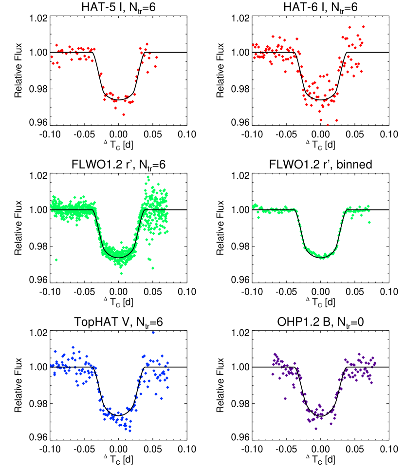
Figure 1.— The five full eclipses examined in this work, with best-fit transit curves over-plotted. The figure in the electronic edition is color-coded according to the bandpass used.

Table 4 Parameters from simultaneous fit of transit curves.

Parameter	Best-Fit Value
$R_{\rm P}$($R_{\rm J}$)	1.154 $\pm 0.032$
$i_{\rm P}$(°)	85.79 $\pm 0.24$
$M_{*}$($M_{\sun}$)	0.82 $\pm 0.03$
$R_{*}$($R_{\sun}$)	0.758 $\pm 0.016$
Period (days)	$2.218573\pm 0.000020$
$T_{0}$ (HJD)	$2453629.39420\pm 0.00024$

To determine the best-fit radius for the planet, we evaluate the $\chi^{2}$ function over all full transits simultaneously, using the same values for the planetary radius and inclination. For this purpose, we employed the downhill simplex minimization routine (amoeba) from Press et al. (1992). The full transits and the fitted curves are exhibited on Fig. 1, the transit parameters are listed in Table 4. In order to determine the $1\sigma$ errors, we fit for the inclination and the radius of the planet using the $1\sigma$ values for the mass and radius of the star (assuming they are uncorrelated). We find that the mass of the star contributes errors of $\pm 0.004$ $R_{\rm J}$ and $\pm 0.12$°, and the radius of the star contributes errors of $\pm 0.032$ $R_{\rm J}$ and $\pm 0.21$°. Using a bootstrap Monte Carlo method, we also estimate the errors from the scatter in our data, and find that this scatter contributes an error of $\pm 0.005$ $R_{\rm J}$ and $\pm 0.03$° to the final measurement. This gives us a total error of $\pm 0.032$ $R_{\rm J}$ for the planet radius and $\pm 0.24$° for the inclination.

Our best-fit parameters gave a reduced $\chi^{2}$ value of 1.23. The excess in the reduced $\chi^{2}$ over unity is the result of our method for normalizing the relative errors for data taken at $N_{tr}=6$, where the RMS variation in the data increases significantly towards the end of the data set, as the source moved closer to the horizon. For these data we define our errors as the standard deviation of the data before the transit, where the scatter was much smaller. This is justified because we know from several sources (night webcamera, raw photon counts) that the conditions were similar (photometric) before and during the transit, and the errors before the transit better represent those inside the transit. This underestimates the errors for data after the transit, inflating the $\chi^{2}$ function accordingly. We find that when we exclude the FLWO1.2 data after the end of the transit (the FLWO1.2 data contain significantly more points than any other single data set), the reduced $\chi^{2}$ for the fit decreases to 0.93.

The results of the planet transit fit are shown in Table 4. The value for the radius of the planet $R_{\rm P}=1.15\pm 0.03$ $R_{\rm J}$ is smaller than the B05 value ($R_{\rm P}=1.26\pm 0.03$ $R_{\rm J}$), and the inclination of $85.8\pm 0.2$° is slightly larger than the B05 value ($85.3\pm 0.1$°). Although our errors are comparable to the errors given by B05, despite the superior quality of the new data, we note that this is a direct result of the larger error ($\pm 0.016$ instead of $\pm 0.01$) for the stellar radius we use in our fits. As discussed in §3.1, we feel that this error, which is based on the effective temperature and bolometric magnitude of the star, is a more accurate reflection of the uncertainties in the measurement of the radius of the star. We note that the errors are dominated by the uncertainties in the stellar parameters (notably $R_{*}$).

Fitting with unconstrained stellar radius

We note that when we fit for the stellar radius directly from the transit curves (meaning we fit for the planet radius, orbital inclination, and stellar radius, but set the stellar mass equal to $0.82$ $M_{\sun}$), we measure a stellar radius of $0.678\pm 0.015$ $R_{\sun}$ and planet radius of $R_{\rm P}=0.999\pm 0.026R_{\rm J}$. The errors for these measurements are from a bootstrap Monte Carlo analysis, and represent the uncertainties in our data alone. To obtain the formal errors, we incorporate the error from the mass of the star and find errors of $\pm 0.017R_{\sun}$ and $0.029R_{\rm J}$, respectively. This means that our data prefer a significantly smaller stellar radius (and a correspondingly smaller planet radius) than our estimates based on temperature, bolometric magnitude, and V-K colors alone would lead us to expect, or a radius smaller than the 0.82$M_{\sun}$ stellar mass implies.

With many more points (869 as compared to $\sim 100$ in the other data-sets) and lower photon-noise uncertainties, the FLWO1.2 data dominate the fit of Eq. 3. However, we repeated our fit with and without these data, and found that the best-fit radius for the star decreased only slightly (to 0.666 $R_{\sun}$) when the FLWO1.2 data were excluded from the fit. Thus, our I, V, and B-band data independently yield values for the stellar radius similar to those implied by the FLWO1.2 data.

The effect of systematic errors

The $\chi^{2}$ minimization formula (Eq. 3) assumes independent noise, and the presence of covariance in the data (due to systematics in the photometry) means that too much weight may be given to a dataset having small formal errors and a great number of datapoints (e.g. the FLWO1.2 data) compared to the other independent data sets (e.g. other telescopes and filters). This is especially a concern when the datasets yield different transit parameters, and one needs to establish whether this difference is significant. In order to follow-up this issue, we repeated the global fit by assuming that the photometric systematics were dominant in the error budget on the parameters – as suggested by our experience with milli-magnitude rapid time-series photometry. We estimated the amplitude of the covariance from the variance of 20-minute sliding averages on the residuals around the best-fitting transit light-curve for each night following the method of Pont (2005). The fit was repeated using these new weights (listed in Table 2, $\sigma_{sys}$), and the resulting parameters (planetary radius, inclination) were within 1% of the values found assuming independent noise. The dispersion of these parameters from the individual nights were found to be compatible with the uncertainties due to the systematics. The amplitude of the systematics is also sufficient to account for the difference in the best-fit stellar radius if it is left as a free parameter. Therefore, with the amplitude of the covariance in the photometry determined from the data itself, we find that the indications of discrepancy between the different data sets and with the assumed primary radius are not compelling at this point.

3.3. Ephemerides

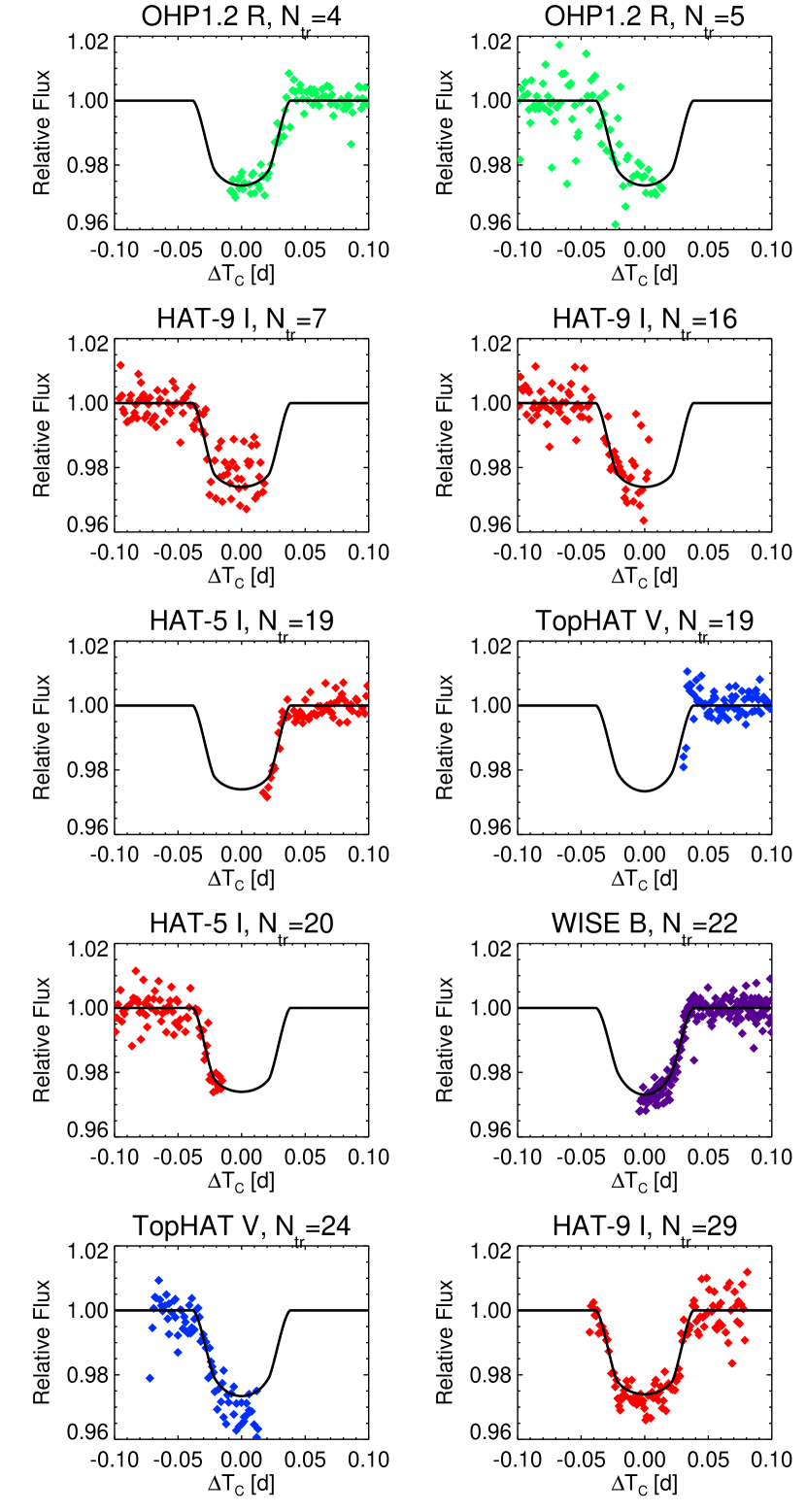
Figure 2.— The ten partial eclipses examined in this work, with best-fit transit curves over-plotted. The eclipses are listed sequentially by date, from top left to bottom right. These eclipses were not used in the fit for the planet radius, inclination, stellar mass, and stellar radius. The figure in the electronic edition is color-coded according to the bandpass used.

Table 5Best-Fit Transit Locations

Telescope	$N_{T}$	$T_{C}$	$\sigma_{\textrm{HJD}}$	(O-C)	$\frac{\textrm{(O-C)}}{\sigma_{\textrm{HJD}}}$
		(HJD, days)	(days)	(days)
OHP1.2	0	2453629.39073	$\pm 0.00059$	$-0.0035$	$-5.9$
OHP1.2	4	2453638.26885	$\pm 0.00067$	0.00035	0.53
OHP1.2	5	2453640.48706	$\pm 0.00174$	$-0.0000079$	$-0.0045$
FLWO1.2	6	2453642.70592	$\pm 0.00022$	0.00029	1.24
HAT-5	6	2453642.70641	$\pm 0.00092$	0.00077	0.84
HAT-6	6	2453642.70649	$\pm 0.00049$	0.00085	1.7
TopHAT	6	2453642.70536	$\pm 0.00048$	$-0.00028$	$-0.57$
HAT-9	7	2453644.92720	$\pm 0.00111$	0.0030	2.7
HAT-9	16	2453664.89287	$\pm 0.00108$	0.0015	1.4
HAT-5	19	2453671.54999	$\pm 0.00113$	0.0029	2.6
TopHAT	19	2453671.54849	$\pm 0.00096$	0.0014	1.5
HAT-5	20	2453673.76725	$\pm 0.00072$	0.0016	2.2
Wise	22	2453678.20080	$\pm 0.00050$	$-0.0020$	$-4.0$
TopHAT	24	2453682.63715	$\pm 0.00100$	$-0.0028$	$-2.8$
HAT-9	29	2453693.73327	$\pm 0.00090$	0.00045	0.51

Note. — These are the best-fit locations for the centers of the fifteen full and partial eclipses examined in this work. We also give the number of elapsed transits $N_{T}$ and O-C residuals for each eclipse.

The transit curves derived from the full-transits for each bandpass were used in turn to calculate the ephemerides of HD 189733 using all transits that have significant OOT and in-transit sections present (for reference, see Table 2). For each transit (full and partial), the center of transit $T_{C}$ was determined by $\chi^{2}$ minimization. Partial transits with the fitted curve overlaid are exhibited on Fig. 2. Errors were assigned to the $T_{C}$ values by perturbing $T_{C}$ so that $\chi^{2}$ increases by unity. The individual $T_{C}$ transit locations and their respective errors are listed in Table 5. The typical timing errors were formally of the order of 1 minute. This, however, does not take into account systematics in the shape of the light-curves. The errors in $T_{C}$ can be estimated from the simultaneous transit observations, for example the $N_{tr}=6$ event was observed by the FLWO1.2m, HAT-5, HAT-6 and TopHAT telescopes (Table 2) and the rms of $T_{C}$ around the median is $\sim 50$ seconds, which is in harmony from the above independent estimate of 1 minute. We applied an error weighted least square minimization on the $T_{C}=P\cdot N_{tr}+E$ equation, where the free parameters were the period $P$ and epoch $E$. The refined ephemeris values are listed in Table 4. They are consistent with both those derived by B05 and by Hébrard & Lecavelier Des Etangs (2006) using Hipparcos and OHP1.2 data, to within $1\sigma$ using our error bars.

We also examined the Observed minus Calculated (O-C) residuals, as their deviation can potentially reveal the presence of moons or additional planetary companions (Holman & Murray, 2005; Agol et al., 2005). The O-C values are listed in Table 4, and plotted in Fig. 3. Using the approximate formula from Holman & Murray (2005), as an example, a 0.15$M_{\rm J}$ perturbing planet on a circular orbit, at 2 times the distance of HD 189733b ($P\approx 6.3^{d}$) would cause variations in the transit timings of 2.5 minutes. The radial velocity semi-amplitude of HD 189733 as induced by this hypothetical planet would be 19m/s, which would be barely noticeable (at the $1\sigma$ level) from the discovery data having residuals of 15m/s and spanning only 30 days.

A few, seemingly significant outlier points on the O-C diagram are visible, but we believe that it would be premature to draw any conclusions, because: i) the error-bars do not reflect the effect of systematics, and for example the $T_{C}$ of the $N_{tr}=0$ OHP discovery data moved by $\sim 5$ minutes after re-calibration of that dataset, ii) all negative O-C outliers are B or V-band data, which is suggestive of an effect of remaining color-dependent systematics. The significance of a few outliers is further diminished by the short dataset we have; no periodicity can be claimed by observing 2 full and 9 partial transits altogether.

According to the theory, the nature of perturbations would be such that they appear as occasional, large outliers. Thus, the detection of potential perturbations also benefits from the study of numerous sequential transits, for example, the MOST mission with continuous coverage and uniform data would be suitable for such study (Walker et al., 2003). We also draw the attention to the importance of observing full transits, as they improve the $T_{C}$ center of transit by a significant factor, partly because of the presence of ingress and egress, and also due to a better treatment of the systematics.

If a planet is perturbed by another planet, the transit-time variations $\Delta t$ are proportional to the period $P$ of the perturbed planet (Holman & Murray, 2005). Although HD 189733b is a relatively short period ($2.21^{d}$) planet compared to e.g. HD 209458b ($3.5^{d}$), it is a promising target for detecting transit perturbations in the future, because the mass of the host star is low and $\Delta t\propto 1/M_{*}$, plus the deep transit of the bright source will result in very precise timing measurements. Observations spanning several months to many years may be needed to say anything definite about the presence or absence of a periodic perturbation.

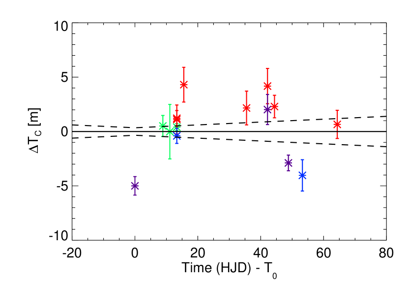
Figure 3.— The residuals calculated using the period and $T_{0}$ derived in this work. The dashed lines are calculated from the uncertainties in the measurements of P and $T_{0}$. The figure in the electronic edition is color-coded according to the bandpass used.

4. Conclusions

Our final values for the planet radius and orbital inclination were derived by fixing the stellar radius and mass to independently determined values from B05 and Masana et al. (2006). We analyzed the dataset in two ways: by $\chi^{2}$ minimization assuming independent errors, and also by assuming that photometric systematics were dominant in the error budget. Both methods yielded the same transit parameters within 1%: if we assume there is no additional unresolved close-in stellar companion to HD 189733 to make the transits shallower, then we find a planet radius of $1.154\pm 0.032R_{\rm J}$ and an orbital inclination of $85.79\pm 0.24\arcdeg$ (Table 4). The uncertainty in $R_{\rm P}$ is primarily due to the uncertainty in the value of the stellar radius.

Figure 4.— Mass-radius diagram depicting known transiting exoplanets, plus Saturn and Jupiter (for comparison). Both the discovery (B05, small filled square) and revised radius (large filled square) for HD 189733 is shown. Sources for the mass and radius values (in this order) are listed after the name of the planet; HD 209458b: Laughlin et al. (2005), Knutson et. al. 2006, in preparation, HD 189733: B05; this paper, OGLE 111b: Pont et al. (2004), OGLE 10b: Konacki et al. (2005), Santos et al. (2006), OGLE 132b: Moutou et al. (2004), OGLE 56b: Torres et al. (2004), OGLE 113b: Bouchy et al. (2004) TrES-1: Laughlin et al. (2005) HD 149026: Sato et al. (2005), Charbonneau et al. (2006).

We note that the TopHAT V-band full and partial transit data, as well as the Wise partial B-band data appear slightly deeper than the best fit to the analytic model. The precision of the dataset is not adequate to determine if this potential discrepancy is caused by a real physical effect (such as a second stellar companion) or to draw further conclusions.

When compared to the discovery data, the radius decreased by 10%, and HD 189733b is in the mass and radius range of “normal” exoplanets (Fig. 4). The revised radius estimate is consistent with structural models of hot Jupiters that include the effects of stellar insolation, and hence it does not require the presence of an additional energy source, as is the case for HD 209458b. On the mass–radius diagram HD 209458b remains an outlier with anomalously low density. We note that the parameters of OGLE-10b are still debated (Konacki et al., 2005; Holman et al., 2006; Santos et al., 2006), but according to the recent analysis of Santos et al. (2006), it also has anomalously low density. With its revised parameters, HD 189733b is quite similar to OGLE-TR-132b (Moutou et al., 2004). The smaller radius leads to a higher density of $\sim 1\rm g\,cm^{-3}$ as compared to the former $\sim 0.75\rm g\,cm^{-3}$. The smaller planetary radius increases the 16µm brightness temperature $T^{(16\mu)}=1117\pm 42\rm K$ of Deming et al. (2006) to $1279\pm 90$K, which is slightly larger than that of TrES-1 and HD 209458b.

We also derived new ephemerides, and investigated the outlier points in the O-C diagram. We have not found any compelling evidence for outliers that could be due to perturbations from a second planet in the system. We note however, that due to the proximity and brightness of the parent star, as well as the deep transit, the system is well suited for follow-on observations.

References

- Agol et al. (2005) Agol, E., Steffen, J., Sari, R., & Clarkson, W. 2005, MNRAS, 359, 567
- Cox (2000) A. N. Cox. 2000, Allen’s astrophysical quantities, 4th ed. Publisher: New York: AIP Press; Springer, 2000
- Bakos et al. (2002) Bakos, G. Á., Lázár, J., Papp, I., Sári, P., & Green, E. M. 2002, PASP, 114, 974
- Bakos et al. (2004) Bakos, G. Á, Noyes, R. W., Kovács, G., Stanek, K. Z., Sasselov, D. D., & Domsa, I. 2004, PASP, 116, 266
- Bakos et al. (2006) Bakos, G. Á. et al. , ApJ, In Press
- Baraffe et al. (1998) Baraffe, I., Chabrier, G., Allard, F., & Hauschildt, P. H. 1998, A&A, 337, 403
- Baraffe et al. (2005) Baraffe, I., Chabrier, G., Barman, T. S., Selsis, F., Allard, F., & Hauschildt, P. H. 2005,A&A, 436, L47
- Bessell et al. (1998) Bessell, M.S., Castelli, F., & Plez, B. 1998, A&A, 333, 231
- Bouchy et al. (2004) Bouchy, F., Pont, F., Santos, N. C., Melo, C., Mayor, M., Queloz, D., & Udry, S. 2004, A&A, 421, L13
- Bouchy et al. (2005) Bouchy, F., et al.2005, A&A, 444, L15
- Carpenter (2005) Carpenter, J. 2005, ApJ, 121, 2851
- Charbonneau et al. (2006) Charbonneau, D., et al. 2006, ApJ, 636, 445
- Claret (2000) Claret, A. 2000, A&A, 363, 1081
- Cutri et al. (2000) Cutri, R. M., et al. 2000, Explanatory Supplement to the 2MASS Second Incremental Data Release (Pasadena: Caltech)
- Cutri et al. (2003) Cutri, R. M., et al. 2003, VizieR Online Data Catalog, 2246,
- Deming et al. (2006) Deming, D., Harrington, J., Seager, S., Richardson, L. J. 2006, astro-ph/0602443
- Gilliland & Brown (1988) Gilliland, R. L., & Brown, T. M. 1988, PASP, 100, 754
- Girardi et al. (2002) Girardi, L. et al. 2002, A&A, 391, 195
- Hébrard & Lecavelier Des Etangs (2006) Hébrard, G., & Lecavelier Des Etangs, A.2006, A&A, 445, 341
- Holman & Murray (2005) Holman, M. J., & Murray, N. W.2005, Science, 307, 1288
- Holman et al. (2006) Holman, M. J., Winn, J. N., Stanek, K. Z., Torres, G., Sasselov, D. D., Allen, R. L., Fraser, W., astro-ph/0506569
- Kervella et al. (2004) Kervella, P., Thévenin, Di Folco, E., & Ségransan, D. 2004, A&A, 426, 297
- Konacki et al. (2004) Konacki, M., et al. 2004, ApJ, 609, L37
- Konacki et al. (2005) Konacki, M., Torres, G., Sasselov, D. D., & Jha, S. 2005, ApJ, 624, 372
- Landolt (1992) Landolt, A. U. 1992, AJ, 104, 340
- Laughlin et al. (2005) Laughlin, G. et al. 2005, ApJ, 621, 1072
- Mandel and Agol (2002) Mandel, K., & Agol, L. 2002, ApJ, 580, L171
- Masana et al. (2006) Masana, E., Jordi, C., Ribas, I. 2006, astro-ph/0601049
- Mason et al. (2001) Mason, B. D., Wycoff, G. L., Hartkopf, W. I., Douglass, G. G., & Worley, C. E. 2001, AJ, 122, 3466
- Moutou et al. (2004) Moutou, C., Pont, F., Bouchy, F., & Mayor, M. 2004, A&A, 424, L31
- Newberry (1991) Newberry, M. V. 1991, PASP, 103, 122
- Perryman et al. (1997) Perryman, M. A. C., et al. 1997, A&A, 323, L29
- Pont et al. (2004) Pont, F., Bouchy, F., Queloz, D., Santos, N. C., Melo, C., Mayor, M., & Udry, S. 2004, A&A, 426, L15
- Pont et al. (2005) Pont, F., Bouchy, F., Melo, C., Santos, N. C., Mayor, M., Queloz, D., & Udry, S. 2005, A&A, 438, 1123
- Pont (2005) Pont, F. 2005, astro-ph/0510846
- Press et al. (1992) Press, W. H., Teukolsky, S. A., Vetterling, W. T., & Flannery, B. P. 1992, Numerical Recipes (2d ed.; London: Cambridge Univ. Press
- Santos et al. (2006) Santos, N. C. 2006, astro-ph/0601024
- Sato et al. (2005) Sato, B., et al. 2005, ApJ, 633, 465
- Skrutskie et al. (2000) Skrutskie, M. F., et al. 2000, VizieR Online Data Catalog, 1, 2003
- Stetson (1987) Stetson, P. B. 1987, PASP, 99, 191
- Tody (1993) Tody, D. 1993, ASP Conf. Ser. 52: Astronomical Data Analysis Software and Systems II, 52, 173
- Tody (1986) Tody, D. 1986, Proc. SPIE, 627, 733
- Torres et al. (2004) Torres, G., Konacki, M., Sasselov, D. D., & Jha, S. 2004, ApJ, 609, 1071
- Udalski et al. (2002a) Udalski, A. et al. 2002a, Acta Astronomica, 52, 1
- Udalski et al. (2002b) Udalski, A. et al. 2002b, Acta Astronomica, 52, 115
- Udalski et al. (2002c) Udalski, A. et al. 2002c, Acta Astronomica, 52, 317
- Young (1967) Young, A. T. 1967, AJ, 72, 747
- Walker et al. (2003) Walker, G., et al.2003, PASP, 115, 1023