The non-linear behavior of the black hole system GRS 1915+105

Abstract

Using non-linear time series analysis, along with surrogate data analysis, it is shown that the various types of long term variability exhibited by the black hole system GRS 1915+105, can be explained in terms of a deterministic non-linear system with some inherent stochastic noise. Evidence is provided for a non-linear limit cycle origin of one of the low frequency QPO detected in the source, while some other types of variability could be due to an underlying low dimensional chaotic system. These results imply that the partial differential equations which govern the magneto-hydrodynamic flow of the inner accretion disk, can be approximated by a small number ( $\approx 3-5$) of non-linear but ordinary differential equations. While this analysis does not reveal the exact nature of these approximate equations, they may be obtained in the future, after results of magneto-hydrodynamic simulation of realistic accretion disks become available.

1. Introduction

Black hole X-ray binaries exhibit variability on a wide range of timescales ranging from months to milli-seconds. This variability is expected to provide important clues about the geometry and structure of these high energy sources. Moreover, a detailed study of the phenomena may eventually be used to test the relativistic nature of these sources and to understand the physics of the accretion process.

The standard first step to quantify variability is to compute the power spectrum which is the amplitude squared of the Fourier transform of the light curve. The power spectra is expected to give information about characteristic frequencies of the system which might show up either as spectral breaks or as near Gaussian peaks, i.e Quasi-Periodic Oscillations (QPO) (e.g. Belloni et al., 2001; Tomsick & Kaaret, 2001; Rodriguez et al., 2002). The shape of the power spectra, combined with the observed frequency dependent time lags between different energy bands, have put constraints on the radiative mechanism and geometry of the emitting region (e.g. Nowak et al., 1999; Misra, 2000; Cui, 1999; Poutanen & Fabian, 1999; Nobili et al., 2001).

The accretion disk which powers these sources maybe undergoing stochastic variations at different length and time scales. This is expected, especially since the viscosity mechanism which drives the accretion process is now believed to be caused by turbulence induced by magnetic instabilities. These structural variations may then manifest as variability in the observed intensity after being convolved with the main radiative process that cools the disk. Additionally, these local stochastic variations could couple resonantly with the global disk structure and produce coherent oscillations. In most analysis, it is implicitly assumed that response of the disk to these fluctuations, either by global resonance and/or radiative processes, is linear in nature. However, there is some evidence that the response of the disk may be non-linear. The ratio of the twin high frequency QPO observed in black hole and neutron star systems, can be explained in a model where the global disk resonates nonlinearly with the stochastic fluctuations (Abramowicz et al., 2003). More compelling model independent evidence has been given by Uttley et al. (2005) (see also Timmer et al. (2000) and Thiel et al. (2001)), who argue that the log-normal distribution of the fluxes and the linear relationship between RMS and flux imply that the response of the disk is non-linear. They show that an exponential response can explain these observations. Earlier Mineshige et al. (1994), had suggested that the behavior of the observed fluctuations could be because the accretion disk is in self-organized critical state. In all these models the temporal behavior of the system is driven by underlying stochastic variations. Moreover, they address the short ($<10$ sec) time-scale variability of the systems, although many systems also exhibit quite dramatic long time-scale variability.

Variability of a system may not necessarily be driven by an underlying stochastic variation. The system can show complicated temporal behavior if the governing differential equations are non-linear and have unstable steady state solutions. In other words, although these systems do not have an explicit time dependent term in the equations describing their structure, they exhibit sustained time variability. In fact, the standard accretion disk theory predicts that the disk is unstable when it is radiation pressure dominated and when the viscous stress scales with the total pressure. Numerical hydro-dynamic simulations reveal that under such circumstances, the disk would undergo large amplitude oscillations around the unstable solution (Chen & Taam, 1994). These variations occur on a viscous time-scale that may be as large as hundreds of seconds. Specific dynamic models for the temporal behavior of accretion disk, like the Dripping Handrail (Young & Scargle, 1996), have been proposed where the apparent random behavior is actually deterministic.

The Galactic micro quasar GRS 1915+105 is a highly variable black hole system. It shows a wide range of long term variability (Chen et al., 1997; Paul et al., 1997; Belloni et al., 1997a) which required Belloni et al. (2000) to classify the behavior in no less than twelve temporal classes. For some classes, low frequency oscillations are observed and the light curves resemble those from numerical simulations of unstable radiation pressure dominated disks based on the standard accretion disk theory. However, the viscosity prescription in the standard disk theory is ad hoc, and while it may represent approximately the time averages viscosity, it is not expected to reproduce the complex time-varying turbulent induced viscosity expected in an accretion disk. Moreover, there could be different types of instabilities in the disk which could give rise to strong variability. Nevertheless, the qualitative similarities between the results of the simulation and observations (Taam et al., 1997), suggests that the long term variability of this source is due to deterministic non-linear evolution of an unstable disk, rather than a manifestation of an underlying stochastic process.

It is important to determine in a more quantitative and general method, whether the long term variability is indeed due to deterministic non-linear behavior rather than having a stochastic origin. That would imply that the temporal behavior of the system can be described by a small number of non-linear ordinary differential equations. In other words, the complex non-linear partial differential equations that are known to govern the hydrodynamical flow, can be approximated by a set of ordinary differential equations and hence can be more easily studied and understood. Such an approximation can be obtained, for example, by studying the non-linear time evolution of a dominant linear mode. This technique which is briefly described in the next section, was used to derive the equations for the well known non-linear Lorenz system. A more physical method is to study the time evolution of spatially averaged quantities as in the one zone approximation by Paczynski (1983) for thermo-nuclear flashes on compact objects. While the rewards of obtaining such approximated equations are far-reaching, these methods are in general not straight forward and require good physical intuition, especially since it is not necessary that they can be obtained for all systems. Hence, evidence for the existence of such an approximation, would give the necessary impetus and direction to the study of these complex systems.

Non-linear time series analysis have been used earlier to analyze X-ray light curves of astrophysical sources. Lehto et al. (1993) used the correlation dimension technique to analyze EXOSAT light curves of several AGN, and found that one, NGC 4051, showed signs of low dimensional chaos. Such analysis have been undertaken on noise filtered Tenma satellite data of Cyg X-1 (Unno et al., 1990) and on EXOSAT data of Her X-1 (Voges et al., 1987; Norris & Matilsky, 1989) and ASCA data of AGN ARK 567 (Gliozzi et al., 2002). In an earlier work, we used a modification of this technique to study RXTE observations of GRS 1915+105 and found evidence that for four of the twelve temporal classes, the system was consistent with harboring a low-dimensional attractor (Misra et al., 2004).

However, a positive result for the correlation dimension analysis, although highly suggestive, is not conclusive evidence that the light curve of these systems is due to a low dimensional chaotic system. The results need to be counter checked using other non-linear techniques and compared with surrogate data analysis. Thus, in this work, we analyze the different temporal patterns exhibited by GRS 1915+105 using correlation dimension analysis and the singular value decomposition technique. For each analysis, we undertake surrogate data analysis as a counter check. To facilitate better physical understanding, we draw analogies between the results obtained for GRS 1915+105 and those for a well known deterministic non-linear system.

It should be emphasized that proving the presence of non-linear dynamics using a finite time series with mathematical certainty is in the very least difficult and perhaps even not a well defined problem. Our motivation here, is not to make model independent and quantitative non-linear diagnosis of the light curve, which as mentioned above is difficult and ambiguous. The goal here is to find out if there are features in the light curve which indicate (but may not necessarily rigorously prove) that the temporal behavior of the black hole system GRS 1915+105, can be described as a set of ordinary non-linear differential equations. Obtaining such equations from first principles would be a major break through in our understanding of accretion disks around black holes and thus any indication that such equations may exist would be useful in formulating them.

In the next section, the well known non-linear system, “Lorenz”, is introduced and some of the different types of non-linear behavior that the system can exhibit are described. In §3, some standard non-linear time series analysis is described and as an example applied to the Lorenz system. In §4, these techniques are applied to the observed light curves of GRS 1915+105 and in §5 the results are summarized and discussed.

2. The Lorenz System

The Lorenz model (Lorenz, 1963) was developed from the Navier-Stokes hydrodynamic equations for the Rayleigh-Bénard flow, which describes the two-dimensional convection of an incompressible fluid in a cell which has a higher temperature at bottom and a lower temperature at top. The essential idea is to choose a dominant linear mode that satisfies the boundary condition, and substitute this mode back into the hydrodynamic equations to obtain the temporal evolution of the mode as a set of ordinary non-linear differential equations. The choice of the dominant mode is rather arbitrary and hence makes this procedure possible only by physical intuition and/or prior knowledge of the solution from experiments or numerical simulations. In spite of the physical (and in particular) hydrodynamical origin of the Lorenz model, it is prudent to be careful about drawing analogies between it and other complex hydrodynamical flows like accretion. For this work, it is sufficient to state that the Lorenz model is a mathematical set of non-linear equations which have been derived from non-linear partial differential equations, using approximations which may or may not be valid. These equations turn out to be

$$\dot{X} = 10(X-Y)$$

$$\dot{Y} = RX-Y-XZ$$

$$\dot{Z} = (8/3)Z-XY$$ (1)

There are three fixed points, or steady state values, of the system: $(X_{o},Y_{o},Z_{o})=(0,0,0)$ and $(\pm\sqrt{[8/3][R-1]},\pm\sqrt{[8/3][R-1]},[R-1])$. $R$ is a control parameter whose value governs the system’s behavior which is obtained by solving numerically these differential equations. For $1<R<14$, the fixed point at the origin is unstable, while the other two are stable. The system evolves towards one of the stable fixed points depending on the initial conditions. The temporal behavior is transitory in nature. For $R>14$, all three fixed points are unstable. For large values of $R>100$, the trajectory along $X$ and $Y$ is a closed loop, called the limit cycle (Left panel of Figure 1). For any initial condition the system evolves towards the limit cycle. For intermediate values of $R$ the behavior of the system is more complex. The right panel of Figure 1 shows the trajectory of $X$ and $Y$ for $R=28$, where the behavior is termed chaotic, i.e. infinitesimally close trajectories diverge exponentially in time. Thus, the Lorenz system can exhibit different types of non-linear behavior.

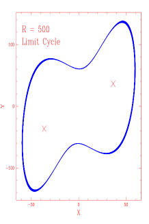
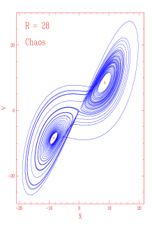
Figure 1.— The Dynamics of the Lorenz system. Left Panel is for $R=500$ showing a limit cycle while the right panel is for $R=28$, when the system exhibits chaos.

Often, in a natural system, only one of the several parameters can be detected and hence the complete dynamic information is not directly available. For example, if only the $X$ variable of the Lorenz system was known, then from the time series for $R=28$ (top panel of Figure 2) and the corresponding power spectrum (bottom panel of Figure 2), the rich complexity of the Lorenz system is not easily identifiable. However, as discussed in the next section, there are non linear techniques by which the complete (qualitative if not quantitative) dynamic nature of such systems can be reconstructed.

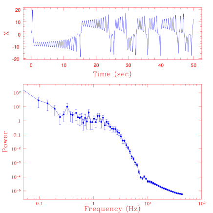
Figure 2.— Top panel: The time series $X(t)$ for the Lorenz system with $R=28$. Bottom Panel: The corresponding power spectrum.

3. Non-linear Time Series Analysis

One of the standard methods to reconstruct the dynamics of a non-linear system from a time series, is the Delay Embedding Technique (Grassberger & Procaccia, 1983). Since the dimension of the system ( i.e. the number of governing equations or variables) is not a priori known, one has to construct the dynamics for different dimensions. In this technique, vectors of length $N$ are created from the time series, $X(t)$, by using a delay time $\tau$, i.e.

$$\vec{v}_{1} = \;\;(X(1),X(2)...X(N))$$

$$\vec{v}_{2} = \;\;(X(1+\tau),X(2+\tau)...X(N+\tau))$$

$$...$$

$$\vec{v}_{M} = \;\;X(1+(M-1)\tau),...X(N+(M-1)\tau)$$ (2)

where $M$ is the chosen dimension. Typically, the delay time $\tau$ is suitably chosen such that the vectors are not correlated i.e. when the auto-correlation function of $X(t)$ approaches zero. For the Lorenz system, such a technique can effectively reconstruct the dynamics as shown in Figure 3, where the $X(t)$ is plotted versus $X(t+\tau)$. Note the similarity between Figures 3 and 1, with the identification of $X(t+\tau)$ with $Y$.

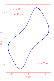
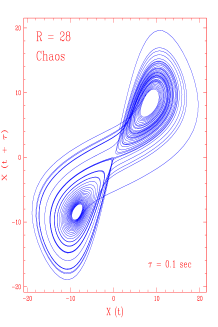
Figure 3.— The reconstructed dynamics of the Lorenz system using the delay embedding scheme. Left Panel is for $R=500$ while the right panel is for $R=28$.

One of the difficulties of this technique is the choice of the appropriate delay time, $\tau$, which in principle depends on the specific nature of the system. To avoid this ambiguity, a modified technique has been proposed by Broomhead & King (1986) where, a matrix constructed of vectors with unit delay time, is decomposed into eigenvectors which then represent the dynamics. Application of this Singular Value Decomposition (SVD) technique to the Lorenz system is shown in the top two panels of Figure 4 which is again qualitatively similar to Figure 1. To generate Figure 4, the time series, $X(t)$ has been converted to a uniform deviate, which is convenient when the analysis is undertaken on data obtained from natural systems (see next section).

To confirm that the dynamical picture obtained by the Delay Embedding technique is indeed due to an underlying deterministic non-linear system and not of stochastic origin, it is customary to compare the results obtained with those of surrogate data (Theiler et al., 1992). Here surrogate data are generated which have practically the same power spectrum and distribution as the original time series, but are of stochastic origin. The essential idea is to formulate a null hypothesis that the data has been created by a stationary linear stochastic process, and then to attempt to reject this hypothesis by comparing results for the data with appropriate realizations of surrogate data. Schreiber & Schmitz (1996) have proposed a scheme, known as Iterative Amplitude Adjusted Fourier Transform (IAAFT), which generates surrogate data that are more consistent in representing the null hypothesis (Kugiumtzis, 1999). In this work, the software which uses tha above technique to generate surrogates (http://www.mpipks-dresden.mpg.de/tisean/TISEAN_2.1/index.html) has been used. The bottom panel of Figure 4, shows the SVD decomposition for surrogate data of the Lorenz system. As expected, the dynamical phase picture is qualitatively different for the surrogate as compared to the original time series. It should be emphasized that a qualitative or quantitative difference between a particular kind of surrogate and original data, although highly suggestive, does not necessarily imply that the original time series has a non stochastic origin. Ideally, the null hypothesis should be tested using several different kinds of surrogate data, before a concrete conclusion can be reached.

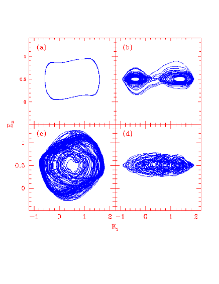
Figure 4.— Singular Value Decomposition (SVD) technique used to reconstruct the Lorenz system dynamics from $X(t)$. (a) Using real data for $R=500$, (b) using real data for $R=28$, (c) using surrogate data for $R=500$ and (d) Using surrogate data for $R=28$.

Data from a natural deterministic non-linear system may have contamination from stochastic noise, either inherently or due to the detection process. Such contamination generally makes it difficult to identify the non-linear behavior of the system. Apart from the level of contamination, the effect on the analysis also depends on the nature of the noise. At the same level of contamination (i.e. at the same percentage of noise addition) the effect of white noise ( i.e. when the power spectrum of the noise signal is a constant) is more than that of red noise ( i.e. when the power spectrum, $P(f)\propto f^{-2}$). This is illustrated in Figure 5, where SVD plots of the Lorenz system with 20% red and white noise addition are shown. While the effect of noise on the limit cycle is to broaden the original one dimensional curve, its effect on the complex chaotic behavior can be more pronounced. Note that a 20% white noise contamination does not allow the dynamics to be effectively reconstructed for the Lorenz system with $R=28$.

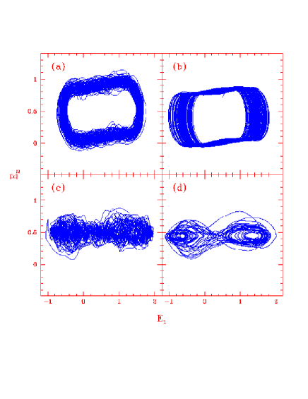
Figure 5.— Singular Value Decomposition (SVD) technique used to reconstruct the Lorenz system dynamics from $X(t)$ with noise contamination at 20% level. (a) Using data for $R=500$ with white noise, (b) using data for $R=500$ with red noise, (c) using data for $R=28$ with white noise and (d) using data for $R=28$ with red noise.

It is often desirable to have a quantitative measure apart from a qualitative picture of the reconstructed dynamics. Such a quantitative measure is the computation of the correlation dimension. Briefly, the computation procedure is to choose a large number of points in the reconstructed dynamics as centers. The correlation function is the number of points which are within a distance R from a center, averaged over all the centers, and may be formally written as

$$C_{M}(R)\equiv\lim_{N\rightarrow\infty}\lim_{N_{c}\rightarrow\infty}{1\over N(N_{c}-1)}\sum_{i}^{N}\sum_{j,j\neq i}^{N_{c}}\hbox{H}(R-|\vec{x}_{i}-\vec{x}_{j}|)$$ (3)

where $\vec{x}_{j}$ are the reconstructed vectors (Eqn 2), $N$ is the number of vectors, $N_{c}$ is the number of centers and H is the Heaviside step function. The fractional or correlation dimension $D_{2}(M)$ is defined as

$$D_{2}(M)\equiv\lim_{R\rightarrow 0}\frac{d\hbox{log}C_{M}(R)}{d\hbox{log}(R)}$$ (4)

and is essentially the scaling index of the variation of $C_{M}(R)$ with $R$. With these definitions, for a finite duration light curve, only an approximate value of $D_{2}(M)$ can be computed. Moreover for small values of $R$, $C_{M}(R)$ is of order unity and hence will not show the intrinsic scaling. Similarly, for large values of $R$, $C_{M}(R)$ will saturate to the total number of data points. Thus for a finite data set, an appropriate scaling region in $R$ needs to be chosen which does not suffer from the above edge effects, to obtain an approximate value of $D_{2}(M)$. Here we use the non-subjective algorithm proposed by Misra et al. (2004) which establishes a region in $R$ which suffers least from edge effect errors and computes $D_{2}(M)$ with an error estimation. A numerical code which implements this algorithm is available at http://www.iucaa.ernet.in/^∼rmisra/NLD.

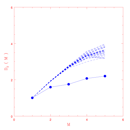
Figure 6.— $D_{2}(M)$ values (filled circles) for the Lorenz system exhibiting chaotic behavior ( $R=28$). The dashed lines represent $D_{2}(M)$ curves for thirty realizations of surrogate data. The $D_{2}(M)$ saturates to $D_{2}^{sat}\approx 2$ and is different from the curves for surrogate data.

For a chaotic system, $D_{2}(M)\approx$ constant $=D_{2}^{sat}$ for $M$ greater than a certain dimension $M_{cr}$. For the Lorenz system exhibiting chaotic behavior (for e.g. when $R=28$), Sprott & Rowlands (2001) have computed using a large number ($N>100000$) points that $D_{2}^{sat}=2.05\pm 0.1$ and $M_{cr}=3$. Figure 6 shows the $D_{2}(M)$ values for the Lorenz system (for $R=28$ using $5000$ points). As expected $D_{2}(M)$ saturates to $D_{2}^{sat}\approx 2$ for $M>M_{cr}\approx 3$. For pure uncorrelated stochastic white noise $D_{2}(M)=M$ for all $M$ and no such saturation exists. However, a saturated value of $D_{2}(M)$ does not necessarily imply that the time series is due to deterministic non-linear behavior. In fact, colored noise (for which the power spectrum $P(f)\propto f^{-\alpha}$) exhibits saturation which can be computed to be $D_{2}^{sat}=2/(\alpha-1)$ (Osborne & Provenzale, 1989). Thus it is necessary to compare $D_{2}(M)$ obtained from the time series with corresponding surrogate data. This is done in Figure 6, where as expected the $D_{2}(M)$ for the Lorenz system is significantly different from the values for the surrogate data. For a deterministic non-linear system the computed $D_{2}^{sat}$ is a quantitative measure of the dynamics and the critical dimension $M_{cr}$ is a measure of the number of equations ( for the Lorenz system $M_{cr}=3$) that are required to describe the behavior. Contamination by noise typically increases the computed $D_{2}(M)$ values and makes it more difficult to distinguish the time series behavior from surrogate data. This is demonstrated in Figure 7, where $D_{2}(M)$ values are plotted for the Lorenz system with different kinds and level of noise contamination.

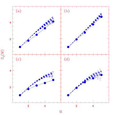
Figure 7.— $D_{2}(M)$ values for the Lorenz system and corresponding surrogate with different levels of white and red noise contamination. (a) 20% white noise, (b) 50% white noise, (c) 20% red noise and (d) 50% red noise.

4. The Black Hole system GRS 1915+105

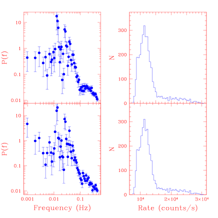
Figure 8.— Top: The power spectrum and the flux ( count rate) distribution for the X-ray light curve of GRS 1915+105 in the $\rho$ state. Bottom: The power spectrum and the flux ( count rate) distribution for corresponding surrogate data.

Based on RXTE observations, Belloni et al. (2001) classified the various temporal behavior of GRS 1915+105 into twelve classes. Here we take a representative data for each class and generate continuous light curves in the energy range $0-30$ keV binned at $1$ sec intervals. The details of the specific data used in the following analysis are tabulated in Misra et al. (2004). Figure 8 shows the power spectrum of the X-ray light curve of GRS 1915+105 when the source is in the $\rho$ state. The presence of a low frequency oscillation with several harmonics is revealed. The flux (or the count rate) distribution during this state has a non Gaussian shape. Although the presence of harmonics of the oscillation and the flux distribution, suggests that the system is non-linear (e.g. Uttley et al., 2005), they do not necessarily imply that this behavior is due to a deterministic non-linear system. The bottom panel of Figure 8 shows the power spectrum and flux distribution for corresponding surrogate data and these are practically indistinguishable from the real case. Thus non-linear time series analysis as described in the previous section is required to ascertain whether the temporal behavior is due to deterministic non-linear behavior.

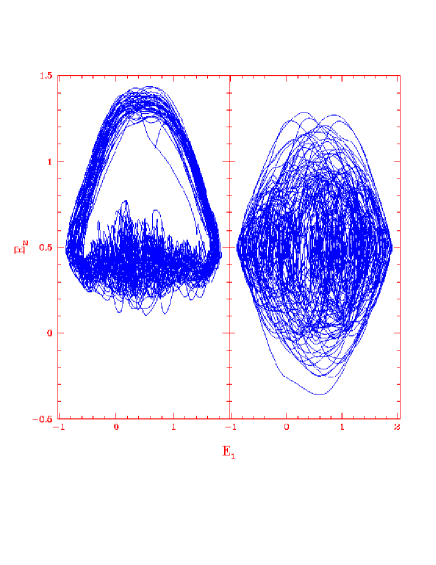
Figure 9.— Singular Value Decomposition (SVD) technique used to reconstruct the dynamics using the X-ray light curve for GRS 1915+105 in the $\rho$ state. Left Panel is for real data while the right panel is for a surrogate data.

The SVD reconstruction of the dynamics for the data is shown in Figure 9. The presence of a main cyclic feature is seen, which is similar to that of the Lorenz system with $R=500$ (Figure 4). This indicates that the observed oscillation is of a limit cycle origin. Note that the surrogate data which has the same power spectrum and distribution has a different SVD reconstruction (Figure 9).

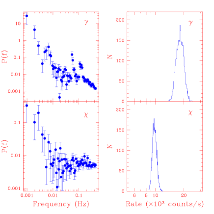
Figure 10.— The power spectrum and the flux (count rate) distribution for the X-ray light curve of GRS 1915+105 in the $\gamma$ and $\chi$ classes.

The power spectra and flux distribution for two other class of GRS 1915+105, $\gamma$ and $\chi$, are shown in Figure 10. A low frequency QPO with harmonics similar to that seen in the $\rho$ class is detected for the $\gamma$ class. During the $\chi$ class no such QPO is detected. However, for both these classes, the SVD reconstruction of the dynamics does not show any qualitative features (Figure 11). Such space filling SVD reconstructions are characteristics of systems with uncorrelated stochastic noise. In agreement with this, the $D_{2}(M)$ values are $\approx M$ and show no saturation, for these two states (Figure 11). Moreover, the $D_{2}(M)$ are consistent with those obtained from corresponding surrogate data. Data from the $\phi$ and $\delta$ classes show similar behavior and are not shown. These results imply that the variability of these classes are of stochastic nature, in contrast to that of the $\rho$ class. In particular, the observed low frequency QPO in the $\rho$ and $\chi$ class have a different origin.

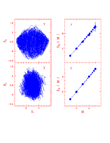
Figure 11.— Left Panels: Singular Value Decomposition (SVD) technique used to reconstruct the dynamics using the X-ray light curve for GRS 1915+105 in the $\gamma$ and $\chi$ classes. Right panels: $D_{2}(M)$ values for the $\gamma$ and $\chi$ classes compared with corresponding surrogates.

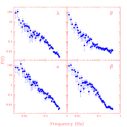
Figure 12.— The power spectra for the X-ray light curve of GRS 1915+105 in the $\lambda$, $\theta$, $\kappa$ and $\beta$ classes.

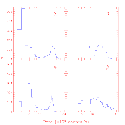
Figure 13.— The flux (count rate) distribution for the X-ray light curve of GRS 1915+105 in the $\lambda$, $\theta$, $\kappa$ and $\beta$ classes.

The behavior of the rest of the classes is more complex. For example, the power spectra for $\lambda$, $\theta$, $\kappa$ and $\beta$ class do not show any strong low frequency periodicity (Figure 12), while the flux distribution is typically non-Gaussian (Figure 13). The SVD reconstruction of these data (Figure 14) show structure which qualitatively maybe similar to that of a chaotic system with noise (Figure 5) and are somewhat different than the SVD reconstruction of the corresponding surrogate data (Figure 15). More evidence is provided by the $D_{2}(M)$ values for these data sets (Figure 16) which show saturation and are different from the values computed from corresponding surrogate data.

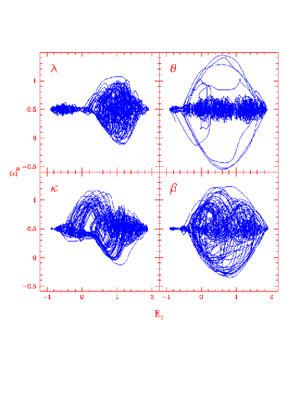
Figure 14.— Singular Value Decomposition (SVD) technique used to reconstruct the dynamics using the X-ray light curve for GRS 1915+105 in the $\lambda$, $\theta$, $\kappa$ and $\beta$ classes.

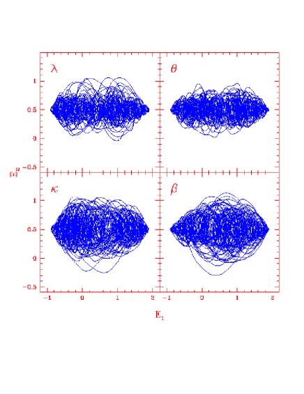
Figure 15.— Singular Value Decomposition (SVD) technique used to reconstruct the dynamics using surrogate data corresponding to the X-ray light curves for GRS 1915+105 in the $\lambda$, $\theta$, $\kappa$ and $\beta$ classes.

Figure 16.— $D_{2}(M)$ values for the $\lambda$, $\theta$, $\kappa$ and $\beta$ classes compared with corresponding surrogates.

5. Summary and Discussion

Using non-linear time series analysis techniques, evidence has been provided that the black hole system GRS 1915+105 exhibits stochastic variability when it is in $\chi$, $\gamma$, $\phi$ and $\delta$ classes. In the $\rho$ class, the low frequency QPO detected in the power spectrum can be attributed to a non-linear limit cycle behavior. For the other classes, the system shows behavior similar to a non-linear chaotic system with some inherent stochastic noise.

Before considering the implications, it is prudent to emphasize that the results presented here need to be confirmed by more comprehensive non-linear data analysis. Since the results are based on a null hypothesis test involving surrogate data, a more comprehensive test should take into account possible different kinds of surrogate data.

The saturation of $D_{2}(M)$ to $D_{2}^{sat}\approx 3-4$ (Figure 16) in analogy with that of the Lorenz system with noise (Figure 7), implies that the temporal behavior of the system is governed by 3-4 underlying global equations. On the other hand, it is believed that the temporal evolution of an accretion disk can be represented by local magneto-hydrodynamic equations which are non-linear differential equations in both time and disk radius. Thus, an encouraging aspect of the results obtained here is that these complicated magneto-hydrodynamic equations may be reducible to (or at least approximated by) a set of simple (although still non-linear) global equations, which are functions of global parameters like size of the disk, average density, pressure etc. Such a set of global equations, will provide a complete picture of the global properties of the inner accretion disk and in principle may enable the testing of general relativity in the strong field limit. However, obtaining these equations from the magneto-hydrodynamic equations directly is challenging. Perhaps spatial averaging of these equations to obtain a one (or two zone) models like as done by Paczynski (1983) may be the most promising option. Such approximations may be obtained with insights gained from the results of future sophisticated numerical magneto-hydrodynamic simulations of realistic accretion disks.

Non-linear time series analysis can also be used to compare results of numerical simulations with real data. If the simulation correctly encompasses the basic non-linear behavior of the system, the resultant simulated light curve should have similar $D_{2}(M)$ values and SVD reconstruction.

In analogy with the Lorenz system, the different temporal behavior (corresponding to the different classes) can be attributed to variation of a single control parameter, which for the Lorenz system is $R$ (Eqn 1). For GRS 1915+105, this controlling parameter could be the time averaged accretion rate, which is determined by the outer boundary condition. One of the key attributes of a deterministic non-linear system is that the time variability need not be due to a time varying parameter. For example, the equations defining the Lorenz system (Eqn 1) do not have an explicit time dependent term. For GRS 1915+105, it is possible that the different temporal classes arise from variations in the accretion rate, while the variability for a given class is due to an inherent non-linearity. Thus it is not necessary to postulate other varying parameters, apart from the accretion rate (like magnetic field etc) to explain the source’s complex variability. If this is true, then the average bolometric luminosity which should be proportional to the average accretion rate, should be different for each class. However, the bolometric luminosity can be estimated only by model dependent spectral fitting with the caveat that the time-averaged spectra may not be adequately represented by steady ones. Nevertheless, the results presented here provide the possibility of identifying a single control parameter which determines the temporal class exhibited by the system.

The temporal behavior of GRS 1915+105 on time-scales of hours and months is unique, but may be related to the state changes that occur for other black hole systems (like Cygnus X-1) on time-scales of months. This difference between GRS 1915+105 and the other black holes has led to the speculation that GRS 1915+105 has a rapidly spinning black hole. Identifying the governing non-linear equations for GRS 1915+105 will not only provide insight into the temporal variability of other black hole systems, but will perhaps give an explanation for its uniqueness.

References

- Abramowicz et al. (2003) Abramowicz, M. A., Bulik, T., Bursa, M., & Kluzniak, W., 2003, A&A, 404, L21.
- Belloni et al. (1997a) Belloni, T., Mendez, M., King, A. R., van der Klis, M., & van Paradijs, J., 1997a, ApJ, 479, L145.
- Belloni et al. (2000) Belloni, T., Klein-Wolt, M., Mendez, M., van der Klis, M., & van Paradijs, J., 2000, A&A, 355, 271.
- Belloni et al. (2001) Belloni, T., Mendez, M., & Sanchez-Fernandez, C., 2001, A&A, 372, 551.
- Broomhead & King (1986) Broomhead, D. S., & King, G. P., 1986, Physica D, 20, 217.
- Chen & Taam (1994) Chen, X., & Taam, R. E., 1994, ApJ, 431, 732.
- Chen et al. (1997) Chen, X., Swank, J. H., & Taam, R. E., 1997, ApJ, 477, L41.
- Cui (1999) Cui, W., 1999, ApJ, 524, 59.
- Gliozzi et al. (2002) Gliozzi, M., et al., 2002, A&A, 391, 875.
- Grassberger & Procaccia (1983) Grassberger, P. & Procaccia, I., 1983, Physica D, 9, 189.
- Kugiumtzis (1999) Kugiumtzis, D., 1999, Phys. Rev. E, 60, 2808.
- Lehto et al. (1993) Lehto, H. J., Czerny, B., & McHardy, I. M., 1993, MNRAS, 261, 125.
- Lorenz (1963) Lorenz, E., N., 1963, J. Atmos. Sci., 20, 130.
- Mineshige et al. (1994) Mineshige, S., Ouchi, N. B., & Nishimori, H., 2004, PASJ, 46, 97.
- Misra (2000) Misra, R., 2000, ApJ, 529, L95.
- Misra et al. (2004) Misra, R., Harikrishnan, K. P., Mukhopadhyay, B., Ambika, G., & Kembhavi, A. K., 2004, ApJ, 609, 313.
- Nobili et al. (2001) Nobili, L., Belloni, T., Turolla, R., & Zampieri, L., 2001, A&Asuppl. , 276 , 217.
- Norris & Matilsky (1989) Norris, J. P., & Matilsky, T. A., 1989, ApJ, 346, 912.
- Nowak et al. (1999) Nowak, M. A., Vaughan, B. A., Wilms, J., Dove, J. B. & Begelman, M. C., 1999, ApJ, 510, 874.
- Osborne & Provenzale (1989) Osborne, A., R., & Provenzale, A., 1989, Physica D., 35, 357.
- Paczynski (1983) Paczynski, B., 1983, ApJ, 264, 282.
- Paul et al. (1997) Paul, B., et al., 1997, A&A, 320, L37.
- Poutanen & Fabian (1999) Poutanen, J., & Fabian, A. C., 1999, MNRAS, 306, L31.
- Rodriguez et al. (2002) Rodriguez, J., Durouchoux, P., Mirabel, I. F., Ueda, Y., Tagger, M., & Yamaoka, K., 2002, A&A, 386, 271.
- Schreiber & Schmitz (1996) Schreiber, T & Schmitz, A., 1996, Phys. Rev. Lett., 77, 635.
- Sprott & Rowlands (2001) Sprott, J. C., & Rowlands, G., 2001, Int. J. Bif. Chaos, 11, 1865.
- Taam et al. (1997) Taam, R. E., Chen, X.,& Swank, J. H., 1997, ApJ, 485, L83.
- Theiler et al. (1992) Theiler, J., et al., 1992, Physica D, 58, 77.
- Thiel et al. (2001) Thiel, M. et al., 2001, A&Asuppl., 276, 187.
- Timmer et al. (2000) Timmer, J., et al., 2000, Phy. Rev. E., 61, 1342.
- Tomsick & Kaaret (2001) Tomsick, J. A., & Kaaret, P., 2001, ApJ, 548, 401
- Unno et al. (1990) Unno, W., et al., 1990, PASJ, 42, 269.
- Uttley et al. (2005) Uttley, P., McHardy, I. M., & Vaughan, S., MNRAS, in press (astro-ph:0502112)
- Voges et al. (1987) Voges, W., Atmanspacher, H., & Scheingraber, H., 1987, ApJ, 320, 794.
- Young & Scargle (1996) Young, K. & Scargle, J. D., 1996, ApJ, 468, 617.