Stellar remnants in galactic nuclei: mass segregation.

Abstract

The study of how stars distribute themselves around a massive black hole (MBH) in the center of a galaxy is an important prerequisite for the understanding of many galactic-center processes. These include the observed overabundance of point X-ray sources at the Galactic center, the prediction of rates and characteristics of tidal disruptions of extended stars by the MBH and of inspirals of compact stars into the MBH, the latter being events of high importance for the future space borne gravitational wave interferometer LISA. In relatively small galactic nuclei, hosting MBHs with masses in the range $10^{5}-10^{7}\,{\rm M}_{\odot}$, the single most important dynamical process is 2-body relaxation. It induces the formation of a steep density cusp around the MBH and strong mass segregation, as more massive stars lose energy to lighter ones and drift to the central regions. Using a spherical stellar dynamical Monte-Carlo code, we simulate the long-term relaxational evolution of galactic nucleus models with a spectrum of stellar masses. Our focus is the concentration of stellar black holes to the immediate vicinity of the MBH. We quantify this mass segregation for a variety of galactic nucleus models and discuss its astrophysical implications. Special attention is given to models developed to match the conditions in the Milky Way nucleus; we examine the presence of compact objects in connection to recent high-resolution X-ray observations.

1. Introduction

Massive black holes (MBHs), with masses ranging from a few $10^{4}\,{\rm M}_{\odot}$ to a few $10^{9}\,{\rm M}_{\odot}$ are probably present in the centers of most galaxies. The most compelling line of evidence is based on measurements of the kinematics of gas and stars in the central regions of nearby galaxies (e.g., Barth 2004; Kormendy 2004; Richstone 2004; Ferrarese & Ford 2005, for recent reviews). The inferred masses of the central dark objects correlate with different properties of the host galaxy, probably most tightly and most fundamentally with the overall velocity dispersion of the spheroidal stellar component of the galaxy ($M-\sigma$ relation, see Gebhardt et al. 2000; Ferrarese & Merritt 2000; Tremaine et al. 2002; Novak et al. 2006). The observational statistics are dominated by systems in which $M_{\bullet}>10^{7}\,{\rm M}_{\odot}$ because kinematic detection of such massive objects is easier to achieve. However, if the $M-\sigma$ relation extends to lower masses, a possibility supported by observations of low-luminosity active galactic nuclei (Greene & Ho 2004; Barth et al. 2005), and most correspondingly small spheroids harbor MBHs, the nuclear MBHs in the $10^{5}-10^{7}\,{\rm M}_{\odot}$ range, of special interest for the present work, may reach a density of order $10^{-2}\,{\rm Mpc}^{-3}$ in the local universe (Aller & Richstone 2002; Shankar et al. 2004).

Our own Milky Way (MW) is the galaxy for which we have the strongest observational evidence for the presence of a central MBH. Spectroscopic and astrometric measurements of the motion of stars in the vicinity of the radio source Sgr A^∗ indeed indicate that they are orbiting a dark mass concentration of some ${3-4}\times 10^{6}\,{\rm M}_{\odot}$ whose average density must exceed ${3}\times 10^{19}\,M_{\odot}\,\mathrm{pc}^{-3}$. This high density is incompatible with a stable cluster of any known less massive astronomical objects (Genzel et al. 2003; Schödel et al. 2003; Ghez et al. 2005), and therefore the presence of a central black hole of the above mass is well accepted. For a comprehensive review of the possible interactions between the Sgr A^∗ MBH and the surrounding stars and their observational consequences, see Alexander (2005).

Mass segregation is thought to bring thousands of stellar BHs in the innermost pc around Sgr A^∗ (Morris 1993; Miralda-Escudé & Gould 2000). This central overpopulation may have a variety of consequences. We note that the compact objects probably dominate the stellar mass density in a region ($R\lesssim 0.1\,$pc) in which the “S” stars are confined (Genzel et al. 2003; Schödel et al. 2003; Ghez et al. 2005). From infrared photometry and spectroscopy, these stars appear to be main sequence (MS) objects with masses of order $4-16\,{\rm M}_{\odot}$ and therefore younger than 100 Myr (Gezari et al. 2002; Ghez et al. 2003; Eisenhauer et al. 2005). This apparent youth in a environment where normal stellar formation is made impossible by the strong tidal forces is an unsolved enigma.

The compact stars may collide and merge with MS stars and giants, hence creating unusual objects, once suggested to be the S-stars themselves (Morris 1993), or increase the rotation rate of extended stars through multiple tidal interactions (Alexander & Kumar 2001). It has also been proposed that S-stars are young stars, formed at $\gtrsim 1$ pc from the MBH, whose orbital eccentricities were increased by some perturbation such as that of an (unseen) stellar cluster, and which were trapped on close orbits around Sgr A^∗ by exchanges with less massive compact remnants (Alexander & Livio 2004).

The presence of the stellar BHs around the MBH can in principle be revealed through different kinds of observations. If one of the objects acts as a secondary gravitational lens for a distant star lensed by the central MBH (Chanamé et al. 2001; Alexander & Loeb 2001; Alexander 2003). Unfortunately, according to these studies, the rate of such double lensing occurring at a detectable level is very low.

If the motions of the S-stars can be tracked with high enough a precision, an extended distribution of non-luminous matter around the Galactic MBH should signal itself through its effect on their orbits. In a slightly non-Keplerian potential, the orbits are affected by Newtonian retrograde precession (Rubilar & Eckart 2001; Weinberg et al. 2005). Present-day observations are insufficient to detect this effect (Mouawad et al. 2005), but Weinberg et al. (2005) have shown that future “extremely large telescopes” (ELTs) with diameters of 30 m or more will likely be able to measure the mass and shape of a dark density cusp of the form $\rho\propto R^{-\gamma}$, if it tallies at least $\sim 2000\,{\rm M}_{\odot}$ within $10^{-2}\,\mathrm{pc}$ of Sgr A^∗ and has $\gamma\leq 2$. This effect is only sensitive to the overall $\rho(R)$; it does not distinguish between a population of stellar BHs and another type of non-luminous component such as a cold dark matter, although the latter probably contributes much less than 10 % of the density inside the innermost pc of the Galaxy (e.g., Gnedin & Primack 2004; Bertone & Merritt 2005a, b). However, if a concentration of $\sim 10\,{\rm M}_{\odot}$ BHs is indeed present, ELT observations should allow us to witness 2-body relaxation at work by the detection of $\sim 3$ gravitational encounters per year between any of $\sim 100$ monitored S-stars and a stellar BH (Weinberg et al. 2005).

Radio pulsars on similar short-period orbits would allow the same kind of measurements with a very high accuracy as well as precise tests of the theory of general relativity (Cordes et al. 2004; Kramer et al. 2004; Pfahl & Loeb 2004). Based on the semi-analytical work of (Miralda-Escudé & Gould 2000), Chanamé & Gould (2002) have suggested that stellar BHs, by concentrating around Sgr A^∗ will push out lighter objects, possibly creating a central dip in their density profile and have pointed out that pulsars would be the ideal probes to detect this effect if the sky position of some 50 of them within a few arcsec of Sgr A^∗ can be obtained. Unfortunately, because of extreme dispersion suffered by radio signals traveling from the Galactic center, the detection of pulsars in this region will probably require future radio telescopes with high sensitivity at frequencies $\gtrsim 10\,$GHz, such as the SKA (Cordes & Lazio 1997; Cordes et al. 2004; Kramer et al. 2004).

Nevertheless, relatively direct evidence for the presence of an abundant population of stellar BHs around Sgr A^∗ may not need to await next-generation telescopes. Recently, observations with the Chandra X-ray satellite have revealed 7 transient sources within 23 pc of projected distance of Sgr A^∗ (Muno et al. 2005b); 4 of them have projected distances smaller than 1 pc, indicative of an overabundance in this central region by a factor $\sim 20$ when normalized to the total enclosed mass at 1 and 23 pc (Launhardt et al. 2002). These sources are believed to be X-ray binaries, i.e., compact objects accreting from a binary companion; however current observations do not shed light on whether these are neutron stars or black holes with low or high mass companions. However, for one case, there is strong evidence for a low-mass ($<1\,{\rm M}_{\odot}$) donor and some preference for a BH accretor (Bower et al. 2005; Muno et al. 2005a; Porquet et al. 2005).

In the present study we undertake a careful numerical model exploration of the distribution of compact objects in galactic centers. Our goal is to assess the importance and detectability of these various effects of mass segregation in the context of existing observations. These models are obtained by explicit integration of the long-term stellar dynamical evolution of spherical nucleus models with account for self-gravity, 2–body relaxation, interactions between stars and the MBH, and, in some cases, additional physics such as large-angle scatterings, collisions or stellar evolution. The models presented here constitute a noticeable improvement over the very few simple estimates of mass segregation available in the literature (Morris 1993; Miralda-Escudé & Gould 2000).

“Extreme-mass-ratio events” (EMREs) in galactic nuclei is our other key motivation. EMREs are events where a stellar object interacts strongly with an MBH. The best studied case so far (first considered by Hills (1975)) is that of an extended star (main sequence or giant) coming so close to the MBH that it is partially or totally disrupted by the intense tidal forces. The hydrodynamical and stellar dynamical aspects of such tidal disruptions have been the object of scores of articles (see references at
http://obswww.unige.ch/$\sim$freitag/MODEST_WG4/TidalDisrupt.html for the former aspect and Frank & Rees 1976; Rees 1988; Magorrian & Tremaine 1999; Syer & Ulmer 1999; Freitag & Benz 2002b; Wang & Merritt 2004, amongst others, for the latter). Although our models also include a simple treatment of tidal disruptions and yield rates for these events, we are more specifically interested in another class of EMRE, namely the coalescence between a compact star and the MBH. “Coalescences” as defined here include “plunges” when a star suddenly finds itself on a radial, relativistically unstable orbit and disappears through the MBH horizon at its next periapse passage, and “inspirals” (EMRIs) during which the orbit of the stellar object progressively shrinks by emission of gravitational waves (GWs) until it plunges.

EMRIs will be of prime interest for LISA (“Laser Interferometer Space Antenna”, see Danzmann 1996, 2000 and http://lisa.jpl.nasa.gov/), the future space borne mission to detect GWs with frequencies in the range $\sim 10^{-4}-0.1$ Hz. The waves emitted during the last year of inspiral, as the stellar object orbits in the deep gravitational field of the MBH, if detected and analyzed successfully, will inform us about the geometry of the space time in the immediate vicinity of the massive object, thus allowing to probe general relativity in the strong field regime, to establish the existence of MBHs and measure with high accuracy their masses and spins (Ryan 1995, 1997; Thorne 1998; Hughes 2003).

Predictions of EMRE rates and properties (especially the mass of stellar object and the orbital eccentricity when the signal starts contributing to the LISA stream) are important for the design and of LISA and the development of data analysis tools required to extract weak EMRE signals from a data stream containing noise and a large number of other astrophysical sources (Phinney 2002; Prince 2002; Gair et al. 2004). For the GW signal to be in the frequency range of optimal LISA sensitivity during the last year of inspiral (when wave amplitude and the interesting strong-field effects are the strongest), the MBH mass must be in the range $M_{\bullet}\simeq 10^{5}-10^{7}\,{\rm M}_{\odot}$. In what follows we argue that such MBHs are likely to inhabit stellar spheroids in which relaxation time is relatively short causing mass segregation close to the MBH. This is of great importance for EMREs as the inspiral a stellar BH, with a mass $\simeq 10\,{\rm M}_{\odot}$ can be detected in galaxies $\sim 10$ times more distant (and therefore $\sim 10^{3}$ more numerous) than that of a $\sim 1\,{\rm M}_{\odot}$ object.

Determining rates and characteristics of EMREs for LISA is beyond the scope of this paper. A few estimates for those exist in the literature, based on the same stellar dynamical code as used here (Freitag 2001, 2003) or on other semi-analytical or numerical methods (Hils & Bender 1995; Sigurdsson & Rees 1997; Miralda-Escudé & Gould 2000; Ivanov 2002; Hopman & Alexander 2005). The results from these studies are scattered over a disquieting large range, approximately from $5\times 10^{-9}\mathrm{yr}^{-1}$ (Hopman & Alexander 2005) to $10^{-6}\mathrm{yr}^{-1}$ (Freitag 2001), for EMRIs of stellar BHs in a MW-like nucleus (see Sigurdsson 2003 for a brief discussion of these various studies and EMRIs in general). This is witness, in part, to the lack of realistic agreed-on models for the structure of galactic nuclei, causing different authors to adopt different approximations and values to describe the stellar distribution around a MBH. With this study, we strive to improve this situation.

Another cause for the disagreement found among EMRI studies is the poor understanding of the mechanisms responsible for EMRIs. All studies have assumed unperturbed spherical galactic nuclei in dynamical equilibrium, in which case 2-body relaxation is certainly the main agent for bringing stars onto very elongated orbits which may result in EMRIs. At the same time, as already pointed out in the pioneering work of Hils & Bender (1995) and analyzed in detail by Hopman & Alexander (2005), encounters with other stars may cause an inspiralling star to plunge prematurely, before its orbital frequency has entered the LISA band. Although GWs emitted during the plunge itself will contain some high-frequency components, it is unlikely to be detectable by LISA as a resolved source because, typically, tens to hundreds of thousands of cycles are required to accumulate enough signal-to-noise ratio (Barack & Cutler 2004a, b; Gair & Wen 2005; Wen & Gair 2005). Hence, for LISA, the problem is not limited to the determination of the rate of coalescences, $\dot{N}_{\rm coal}$; one also needs to compute the fraction of those, $f_{\rm EMRI}\equiv\dot{N_{\rm EMRI}}/\dot{N}_{\rm coal}$, that are “clean” inspirals instead of plunges. However, here, we limit ourselves to $\dot{N}_{\rm coal}$, the quantity for which the type of simulations we carry out yield robust predictions. We think that a real trustworthy estimate of $f_{\rm EMRI}$ can only be arrived at through the use of novel methods, to be developed in the future (see § 5).

The rest of this paper is organized as follows. In § 2, a quick review of the relevant aspects of stellar dynamics in galactic nuclei and the previous relevant work is presented. In § 3, we describe the numerical method used in our simulations, as well as the physics and initial conditions implemented. Our main results from our $\simeq 80$ simulations are described in § 4 and we conclude in § 5 with a discussion of the astrophysical implications of our results and an outlook for future work.

2. Review of the Theory and Previous Studies

2.1. Collisional Dynamics in Galactic Nuclei

In stellar dynamics, the term “collisional” refers to all situations in which the discrete nature of stars, i.e. the fact that a stellar system is not composed of a continuous fluid but of individual objects, plays a role. In the context of galactic nuclei, these effects include 2-body relaxation, direct (hydrodynamical) collisions between stars and close, dissipative interactions between stars and a central MBH.

In this work, we restrict ourselves to the situation of isolated, spherical systems in dynamical equilibrium. These assumptions are made necessary by the numerical method we use (the Monte-Carlo code, see § 3) which is still, at the present day, the only stellar dynamical scheme able to treat the collisional evolution of systems consisting of more than one million stars with acceptable realism. They are also adopted in almost all other works on the subject because they introduce a well-defined theoretical framework, allowing in particular to make use of methods developed for the study of globular clusters. Here we use the term “cluster” for any collisional stellar system, including galactic nuclei. Collisional dynamics, generally with a focus on globular or smaller clusters is covered by several textbooks (Binney & Tremaine 1987; Spitzer 1987; Heggie & Hut 2003); therefore we only recall here the few concepts needed to understand the rest of the paper. More detailed explanations about collisional dynamics in the context of Monte-Carlo simulations can be found in our previous papers (Freitag & Benz 2001, 2002b; Freitag et al. 2006).

Barring the effects of mass loss due to stellar evolution, in a stationary smooth, spherical potential, stellar orbits would be energy- and angular-momentum-conserving rosettes of fixed shape and the cluster structure would show no secular evolution. But the potential is the sum of the contribution of a finite number of stars (and a MBH) and is affected by short-scale and short-time fluctuations which causes the orbital parameters to slowly change. In effect, stars are exchanging energy and angular momentum with one another and, to a very good approximation this “relaxation” can be idealized as due to the sum of a large number of uncorrelated 2-body encounters leading to small deflection angles. This is the base for the Chandrasekhar theory of relaxation (Chandrasekhar 1960) on which the Fokker-Planck equation and other approximate treatment of collisional dynamics are based (Binney & Tremaine 1987; Hénon 1973).

In this picture, one can define a local relaxation time

$$t_{\rm rlx}= \frac{\sqrt{2}\pi}{64}\frac{\sigma^{3}}{\ln\Lambda\,nG^{2}\langle m_{\ast}\rangle^{2}}={3.67}\times 10^{8}\,{\rm yr}\,\times$$

$$\left(\frac{\ln\Lambda}{10}\right)^{-1}\left(\frac{\sigma}{100\,\mathrm{km\,s}^{-1}}\right)^{3}\left(\frac{n}{10^{6}\,\mathrm{pc}^{-3}}\right)^{-1}\left(\frac{\langle m_{\ast}\rangle}{{\rm M}_{\odot}}\right)^{-2}$$

where $\ln\Lambda$ is the Coulomb logarithm, $\sigma$ is the 1D velocity dispersion, $n$ the number density of stars and $\langle m_{\ast}\rangle$ the average stellar mass. The slightly unusual numerical coefficient is devised such that a particle of mass $\langle m_{\ast}\rangle$ traveling for a time $\delta t$ through a field of particles of same mass at a relative velocity $v_{\rm rel}=\sqrt{2}\sigma$ would have its trajectory deflected by an angle $\delta\theta$, with $\langle\delta\theta^{2}\rangle=(\pi/2)^{2}\delta t/t_{\rm rlx}$.

The argument of the Coulomb logarithm is $\Lambda=b_{\rm max}/b_{0}$ where $b_{0}=G\langle m_{\ast}\rangle/\sigma^{2}$ is the typical impact parameter leading to a deflection angle of $\pi/2$ in gravitational encounters between stars. In a virialized, self-gravitating system, $b_{\rm max}$ is of order the half-mass radius $R_{\rm h}$ and $\Lambda=\gamma_{\rm c}N_{\ast}$ with $\gamma_{\rm c}\approx 0.01$ if stars have a mass spectrum (Freitag et al. 2006, and references therein). In the region where the gravitational force is dominated by the central object, one finds $\Lambda\approx M_{\bullet}/\langle m_{\ast}\rangle$ (e.g., Bahcall & Wolf 1976). In practice, this does not lead to an important difference, thanks to the damping effect of the logarithm. For instance, one finds $\ln(\gamma_{\rm c}N_{\ast})\simeq 15$ for $N_{\ast}={3}\times 10^{8}$ and $\ln(M_{\bullet}/\langle m_{\ast}\rangle)\simeq 11.5$ for $M_{\bullet}=10^{5}\,{\rm M}_{\odot}$ and $\langle m_{\ast}\rangle=1\,{\rm M}_{\odot}$. Therefore, in most studies, including the present one, a fixed value of $\Lambda$ ($=\gamma_{\rm c}N_{\ast}$) is adopted. Comparisons with direct $N-$body integrations, presented in § 4.1, as well as with a version of the Monte-Carlo code in which $\Lambda$ varies with the distance to the center, from $M_{\bullet}/\langle m_{\ast}\rangle$ to $\gamma_{\rm c}N_{\ast}$ (Freitag 2000), confirm the validity of this approximation. We set $\gamma_{\rm c}=0.01$.

The MBH dominates the gravitational force acting on stars within an “influence sphere” with a radius of order $GM_{\bullet}\sigma_{0}^{-2}$ where $\sigma_{0}$ is the stellar velocity dispersion at larger distances (a more practical definition is given in § 3.2 for the category of galactic nucleus models considered in our simulations). In this central region, the velocity dispersion is Keplerian, $\sigma(R)\simeq GM_{\bullet}/R$. If the stars are distributed according to a a power-law density profile, $n\propto R^{-\gamma}$, the relaxation time gets shorter closer to the MBH when $\gamma>1.5$ and longer if $\gamma<1.5$.

In what follows, we call “collision” the event in which two stars actually come so close to each other as to touch. Neglecting deformations due to mutual tidal interactions, a collision between stars of radii $r_{1}$ and $r_{2}$ corresponds to their centers coming within a distance $r_{1}+r_{2}$ of each other. The cross section for this process is

$$S_{\rm coll}^{(1,2)}=\pi(r_{1}+r_{2})^{2}\left[1+\frac{2G(m_{1}+m_{2})}{(r_{1}+r_{2})V_{\rm rel}^{2}}\right]$$ (2)

where $m_{1,2}$ are the stellar masses and $V_{\rm rel}$ their relative velocity at a large separation. If field-stars of type “2” have number density $n_{2}$, and all stars of this type have the same velocity, the average time for test-star “1” to collide with one of type “2” is

$$t_{\rm coll}^{(1,2)}=\left(n_{2}S_{\rm coll}^{(1,2)}V_{\rm rel}\right)^{-1}$$ (3)

To estimate the importance of collisions in the dynamics, we assume all stars have the same mass and radius, $m_{\ast}$, $r_{\ast}$ and their velocity distribution is Maxwellian with dispersion $\sigma$. The collision time is then (Binney & Tremaine 1987)

$$t_{\rm coll}= \left[16\sqrt{\pi}n\sigma r_{\ast}^{2}\left(1+\frac{Gm_{\ast}}{2\sigma^{2}r_{\ast}}\right)\right]^{-1}\simeq{8.9}\times 10^{10}\,{\rm yr}\,\times$$ (4)

$$\left(\frac{n}{10^{6}\,\mathrm{pc}^{-3}}\right)^{-1}\left(\frac{\sigma}{100\,\mathrm{km\,s}^{-1}}\right)\left(\frac{r_{\ast}}{{\rm R}_{\odot}}\right)^{-1}\left(\frac{m_{\ast}}{{\rm M}_{\odot}}\right).$$

The numerical relation is valid when the velocities are much smaller than the stellar escape velocity, $\sigma\ll V_{\ast}=(2Gm_{\ast}/r_{\ast})^{1/2}=617.5\,\mathrm{km\,s}^{-1}\,(m_{\ast}/{\rm M}_{\odot})^{1/2}(r_{\ast}/{\rm R}_{\odot})^{-1/2}$ so that the cross section is dominated by gravitational focusing. This ceases to be applicable at distances from the MBH smaller than

$$R_{\rm coll}=r_{\ast}\frac{M_{\bullet}}{m_{\ast}}\simeq{2.3}\times 10^{-2}\,\mathrm{pc}\left(\frac{M_{\bullet}}{10^{6}{\rm M}_{\odot}}\right)\left(\frac{m_{\ast}}{{\rm M}_{\odot}}\right)^{-1}.$$ (5)

For $R<R_{\rm coll}$, $\sigma>V_{\ast}$, so the collision time reduces to (note the different normalization for $n$ and $\sigma$)

$$t_{\rm coll}\simeq {6.7}\times 10^{10}\,{\rm yr}\,\times$$

$$\left(\frac{n}{10^{7}\,\mathrm{pc}^{-3}}\right)^{-1}\left(\frac{\sigma}{10^{3}\,\mathrm{km\,s}^{-1}}\right)^{-1}\left(\frac{r_{\ast}}{{\rm R}_{\odot}}\right)^{-2}.$$

The condition for the collision time to become shorter than the relaxation time is also $\sigma>V_{\ast}$, for $\ln\Lambda\approx 10-20$. Collisions at such velocities are unlikely to lead to mergers; a fly-by with partial mass loss is the most likely outcome (Freitag & Benz 2005). Only within $R_{\rm coll}$ can collisions noticeably affect the density profile (Frank & Rees 1976; Sigurdsson & Rees 1997). However, hydrodynamical simulations of collisions between MS stars show that complete stellar disruptions require $\sigma\gtrsim 5V_{\ast}$ and nearly head-on geometry (Benz & Hills 1987, 1992; Lai et al. 1993; Freitag & Benz 2002a, 2005). Disruptions are therefore rare and the effect of collisions on the stellar distribution is weak, even for $R<R_{\rm coll}$ (Freitag & Benz 2002b).

Gravitational encounters with an impact parameter smaller than a few $b_{0}$ lead to deflection angles that are relatively large and cannot be accounted for in the standard, “diffusive” theory of relaxation. Therefore in most approaches, both analytical and numerical, these large-angle scatterings have to be considered as a separate process. We call them “large-angle scatterings” and reserve the word “relaxation” to the effect of 2-body encounters with larger impact parameters. On average, a star will experience an encounter with impact parameter (with $f_{\rm LA}$ of order a few) over a timescale

$$t_{\rm LA}\simeq\left[\pi(f_{\rm LA}b_{0})^{2}n\sigma\right]^{-1}\approx\frac{\ln\Lambda}{f_{\rm LA}^{2}}t_{\rm rlx}.$$ (7)

The effects of large-angle scatterings on the overall evolution of a cluster are negligible in comparison with “diffusive” relaxation (Hénon 1975; Goodman 1983). However, unlike the latter process, they can produce velocity changes strong enough to eject stars from an isolated cluster (Hénon 1960, 1969; Goodman 1983) or, more importantly, from the “cusp” around the central BH (Lin & Tremaine 1980; Baumgardt et al. 2004a). Therefore they may be important for the dynamics of the innermost regions just where mass segregation is relevant too.

A central MBH represents a sink for the stellar system as it destroys, captures or –if it forms a very compact binary with another object– ejects stars that venture very close to it, i.e., within some distance $R_{\rm loss}$. In particular, tidal disruption, for a star of radius $r_{\ast}$ and mass $m_{\ast}$, occurs at $R_{\rm loss}=R_{\rm t.d.}\simeq 1.25\,r_{\ast}(M_{\bullet}/m_{\ast})^{1/3}$ (Freitag & Benz 2002b, and references therein). A quasi parabolic orbit whose Newtonian periapse distance would be smaller than $R_{\rm loss}=R_{\rm plunge}=8GM_{\bullet}c^{-2}$ actually plunges directly through the horizon (Zeldovich & Novikov 1999). Orbits with periapse distance $<R_{\rm loss}$, corresponding to angular momentum (per unit mass) $J<J_{\rm LC}\simeq\sqrt{2GM_{\bullet}R_{\rm loss}}$, form the “loss cone”. For a star with velocity $v$ at distance $R$ from the center, the loss cone has an aperture angle $\theta_{\rm LC}=J_{\rm LC}/(Rv)$.

If the star is removed from the cluster in a single close encounter with the MBH, a mature loss cone theory has been developed which predicts rates and orbital characteristics of such events (Frank & Rees 1976; Bahcall & Wolf 1977; Lightman & Shapiro 1977; Cohn & Kulsrud 1978; Amaro-Seoane et al. 2004). The notion of critical radius ($R_{\rm cr}$) is central in these cases; it is basically the semi-major axis of an orbit for which the relaxation processes cause a change of angular momentum per orbital time of order $J_{\rm LC}$. Inside $R_{\rm cr}$ loss cone orbits are nearly completely depleted (“empty loss cone” regime). On the scale of the loss cone, the change of orbital parameters due to relaxation can be treated as a diffusion process and a direct analogy with the heat equation can be used to obtain the average time for a star to be destroyed, $t_{\rm destr,e}\simeq\ln(\theta_{\rm LC}^{-2})t_{\rm rlx}$. At distances larger than $R_{\rm cr}$, relaxation is efficient enough to bring stars into and out of the loss cone over an orbital time $P_{\rm orb}$. The loss cone is therefore full and $t_{\rm destr,f}\simeq\theta_{\rm LC}^{-2}P_{\rm orb}$. The total rate of interactions with the MBH is given by $\Gamma=4\pi\int R^{2}nt_{\rm destr}^{-1}dR$. It peaks around $R_{\rm cr}$ for many density profiles $n(R)$.

In cases, such as non-destructive tidal interactions and GW emission, in which the star looses energy gradually and is only destroyed after a large number of periapse passages, the interplay between relaxation and dissipative processes is not directly amenable to the relatively simple loss cone formalism. The detailed analysis of such situations has only recently been pioneered (Alexander & Hopman 2003; Hopman & Alexander 2005).

In the sphere of influence of the MBH, orbits of bound stars are essentially ellipses precessing on a time scale of order $(M_{\bullet}/M_{\ast,orb})P_{\rm orb}\gg P_{\rm orb}$ where $M_{\bullet}$ is the mass of the central object, $M_{\ast,\rm orb}$ the mass in stars within the apocenter distance of the orbit and $P_{\rm orb}$ the orbital period. On shorter timescales, orbits exert torques on each other, thus introducing so-called “resonant relaxation” which affects the angular momentum on a time scale $t_{\rm res}\approx(M_{\bullet}/m_{\ast})P_{\rm orb}\approx\ln\Lambda^{-1}(M_{\bullet}/M_{\ast,orb})t_{\rm rlx}$ (Rauch & Tremaine 1996). Resonant relaxation is suppressed by relativistic precession for very close-by orbits satisfying $R_{\rm peri}/R_{\mathrm{S}}<M_{\bullet}/M_{\ast,orb}$ with $R_{\rm peri}$ the periapse distance and $R_{\mathrm{S}}=2GM_{\bullet}/c^{2}$ the Schwarzschild radius of the central BH. Although resonant relaxation may be much faster than “normal” relaxation in the sphere of influence of the MBH, it was shown to have only a moderate impact on the rate of tidal disruptions in galactic nuclei, because these events are dominated by stars with semi-major axis of order the critical radius (see § 3.2) and $M_{\bullet}/M_{\ast,orb}\ll 10$ (Rauch & Tremaine 1996; Rauch & Ingalls 1998). On the other hand, the effects on the coalescence of compact objects is likely to be weak due to relativistic precession. In any case, the study of this question requires a method that can account for non-local gravitational interactions between orbits (“2-orbit” effects) and is not undertaken here.

2.2. Single-Mass Clusters with a Central Object

The question of how relaxation will shape the distribution of a large number of point-like objects of the same mass orbiting a massive object has been addressed in the 70’s, shortly after the detection of X-ray sources in globular clusters triggered the hypothesis that there may be IMBHs at their center (Peebles 1972; Bahcall & Wolf 1976; Shapiro & Lightman 1976; Lightman & Shapiro 1977; Cohn & Kulsrud 1978). The approximate solution, first found by Bahcall & Wolf (1976) is this context through a Fokker-Planck-type treatment of the stellar dynamics, is the formation of a power-law density, $n(R)\propto R^{-7/4}$. In this simplified treatment, stars are only destroyed if they reach a very high binding energy (typically $E_{\rm loss}\approx GM_{\bullet}/R_{\rm t.d.}$ for tidal disruptions). As it neglects the disruption of stars on (very) elongated orbits ($J<J_{\rm LC}$), this idealized configuration corresponds to an isotropic distribution with a zero net diffusive flux of stars in $E$ space and a constant outward energy flux. More detailed Fokker-Planck treatment accounting for loss-cone effects and other realistic bounding conditions confirmed the Bahcall-Wolf cusp as a very good approximation (Bahcall & Wolf 1977; Lightman & Shapiro 1977; Cohn & Kulsrud 1978). It has since be found with other methods also based on the diffusive, local theory of relaxation: two types of Monte Carlo codes (Shapiro 1985 and references therein; Freitag & Benz 2002b) and a gas-dynamical approach (Amaro-Seoane et al. 2004). Very recently, the approximations involved in these computations have been vindicated by direct $N-$body simulations in which the formation of the $R^{-7/4}$ profile over a relaxation time was indeed witnessed (Baumgardt et al. 2004a; Preto et al. 2004).

Using a homological model for the evolution of a cluster, Shapiro (1977) showed how a central BH can power the expansion of the stellar system, by destroying stars that have diffused deep into the cusp. A central BH is therefore able to drive gravothermal expansion in a way similar to hardening binaries, but without leading to core oscillations (Heggie & Hut 2003). The central BH acts as a heat source for the whole cluster only if, on average, destroyed stars have negative orbital energies relative to the BH, a condition roughly equivalent to $R_{\rm cr}<R_{\rm infl}$ (Duncan & Shapiro 1983).

2.3. Multi-Mass Clusters with a Central Object

Surprisingly, the effects of relaxation in a multi-mass cluster containing a central massive object have been little studied. To our knowledge, the only in-depth theoretical study of mass segregation in the Keplerian potential of a MBH is the work of Bahcall & Wolf (1977). The long-term evolution of a few models of MBH-hosting galactic nuclei with a mass spectrum was followed numerically using a Fokker-Planck code by Murphy et al. (1991) and with the same Monte-Carlo code as the present study by Freitag & Benz (2002b) and Freitag (2003). However, in those studies, rich physics was included which complicates the interpretation of the results (collisions, stellar evolution,…) and their authors did not present detailed results concerning mass segregation. Also, with the exception of Freitag (2003), the initial conditions used were not tailored to represent any specific galactic nucleus. Recently, (Baumgardt et al. 2004b) carried out direct $N-$body simulations of multi-mass clusters with some ${1.6}\times 10^{4}$ to ${1.3}\times 10^{5}$ stars hosting a central IMBH and discussed how stars of different masses distribute themselves around the central object. This study offers the only direct characterization of mass segregation around a massive object. One should be cautious, however when trying to apply these $N-$body results to larger systems such as galactic nuclei because small$-N$ effects (large-angle scatterings, binary interactions, IMBH wandering,…) may play a significant role there (Lin & Tremaine 1980).

A first step towards the understanding of mass segregation in galactic nuclei is to consider the simpler problem of the evolution of one or a few massive “tracers” in a non-evolving stellar background. We undertake this step here for illustrative purposes. This is a useful idealization for the early dynamical evolution of the population of stellar BHs. Those are very rare objects so, until they have concentrated in the innermost regions, they will mostly interact with other stars and not with one another. We assume all stellar BHs have mass $m_{\rm BH}$ and all other stars have mass $m$ with $q=m_{\rm BH}/m\gg 1$; $q=30$ is a realistic value. The effects of 2-body relaxation on the orbit of a massive particle (“test particle”) in a field of much lighter field particles is embodied in the classical dynamical friction (DF) formula (see Binney & Tremaine 1987, § 7.1)

$$\vec{a}_{\rm DF}=-t_{\rm DF}^{-1}\,\vec{v}=-\frac{4\pi\ln\Lambda G^{2}nm(m+m_{\rm BH})}{v^{3}}\kappa(X)\,\vec{v}$$ (8)

with $\kappa(X)={\rm erf}(X)-2\pi^{-1/2}Xe^{-X^{2}}$ and $X=v/(\sqrt{2}\sigma)$. In this formula, $\vec{a}_{\rm DF}$ is the force per unit mass on the test particle due to DF, $\vec{v}$ its velocity, $n$ the density of field particles, and $\sigma$ the (1D) dispersion of their velocities, assumed to have a Maxwellian distribution. $t_{\rm DF}$ is of order the local relaxation time divided by $1+q$ so the massive particles should already experience significant mass segregation after a small fraction of the relaxation time.

For an object on a circular orbit of radius $R$, $v=v_{\rm c}\equiv\sqrt{GM_{\rm encl}(R)/R}$ where $M_{\rm encl}(R)$ is the total mass within $R$, and a differential equation for the evolution of $R$ is easily derived from ${a}_{\rm DF}R=d(Rv)/dt$,

$$\frac{dR}{dt}=-\left(\frac{2\pi GR^{2}n(R)m}{v_{\rm c}(R)^{2}}+0.5\right)^{-1}\frac{R}{t_{\rm DF}(R)}.$$ (9)

Although it can yield a qualitative understanding and a first approximation to the development of mass segregation, a treatment based on the use of Eq. 9 falls short of physical realism. First, relaxation reduces to dynamical friction only in the limit of very large mass ratio. In general, the direction of $\vec{v}$ (and not only its modulus) is also affected by 2-body encounters, causing the eccentricity of a circular orbit to drift away from zero. Second, if massive objects are numerous enough, they will eventually come to dominate the central region. There, they will push the lighter objects away by heating them and start interacting with each other in a way more similar to the single-mass situation. The dynamical friction picture does not provide a way to determine the quasi-stationary distribution the particles of different masses will adopt on the long term.

In another seminal paper, Bahcall & Wolf (1977) studied the possibility for a multimass system dominated by the potential of a central MBH to settle into a relaxational steady-state configuration (a cusp), provided stars lost to interactions with the MBH are replaced by stars coming from more distant regions. By solving the coupled Boltzmann equations for stars of various masses, they found that the stars of different masses, $m_{i}$, should approximately follow one-particle distribution functions that are power law of the binding energy, $f_{i}(\vec{x},\vec{v})=F_{i}(E)\propto E^{p_{i}}$, with indices scaling like

$$\frac{p_{i}}{m_{i}}=\frac{p_{j}}{m_{j}}.$$ (10)

These correspond to density profiles $n_{i}\propto R^{-\gamma}$ with $\gamma=\frac{3}{2}+p$. They found $p\simeq 0.30$ for the most massive objects, who dominate the central density, close to the value for a single-mass distribution, $p\simeq 0.25$. For much lighter objects in the innermost regions, $\gamma\simeq 1.5$ is expected (see also Merritt 2004).

It is interesting to note that the massive stars concentrate to the center because they lose energy to lighter ones during 2-body encounters. This tendency would yield statistical equipartition of kinetic energy if it wasn’t for the overall gravitational potential in which the heavy objects sink, thus increasing their velocities. In a cluster without a central black hole, equipartition can only be reached at the center and only if the massive particles are in small number or have a mass not much exceeding that of the lighter ones, so that they cannot form a self-gravitating system, with negative heat capacity, on their own (Spitzer 1969; Vishniac 1978; Inagaki & Saslaw 1985; Watters et al. 2000; Gürkan et al. 2004; Khalisi et al. 2005). For all realistic mass spectrum, mass segregation will trigger the core collapse of the sub-system of massive bodies, a process known as “Spitzer instability”.

Clearly, in a fixed Keplerian potential, massive stars can never reach equipartition with lighter ones; as they concentrate to the center, their velocity dispersion must increase and the thermal imbalance with the lighter objects is maintained. An accelerated, catastrophic collapse of the population of massive objects is prevented, however, by the heating effect of the central MBH which eventually compensates for the energy lost to the light stars. Hence, a cusp of massive objects is expected to form and maintain itself in thermal quasi equilibrium while it drives the expansion of the distribution of lighter objects.

Published simulations of multi-mass clusters with a central (I)MBH are few and far apart. The work of Murphy et al. (1991) stands out as a pioneering effort to follow the evolution of galactic nuclei taking into account relaxation, stellar evolution and collisions. These authors have published limited data from one run without stellar evolution or collisions. They report a good agreement with the prediction of Bahcall & Wolf (1977) relative to the cusp exponents for stars of different masses (Eq. 10). From their Figure 9, however, it seems that the region for which this applies encompasses of order $10^{4}\,{\rm M}_{\odot}$ only, at a time when, judging from their case 4C, the MBH has certainly grown past $10^{6}\,{\rm M}_{\odot}$.

To our knowledge, Baumgardt et al. (2004b) have presented the only direct $N-$body simulations of a multi-mass system with a central massive object. Although they observe that the most massive objects form a power-law cusp of exponent compatible with $\gamma=1.75$, the central profiles of the lighter species are found to be much shallower than predicted by Eq. 10, with $\gamma\simeq 0.75+m_{\ast}/(1.1\,{\rm M}_{\odot})$. However, in the light of our comment on Murphy et al. (1991) and of our simulations, this cannot be interpreted as a rebuttal of Bahcall & Wolf (1977) but more likely is an indication that the appropriate regime is only reached deep in the influence region, a region not probed by $N-$body simulations with $N_{\rm p}\lesssim 131\,000$.

3. Simulations: Method and Initial Conditions

3.1. The Monte-Carlo Code for Nucleus Dynamics

This work is based on simulations of the long-term stellar dynamical evolution of galactic nuclei performed with ME(SSY)$\ast\ast$2. This code is based on the Monte-Carlo algorithm first described and implemented by Hénon (Hénon 1971b, a, 1973, 1975). It has been described in detail by Freitag & Benz (2001, 2002b). Here, we succinctly remind the basics of the method and the included physics.

The Monte-Carlo method is based on the assumptions of spherical symmetry and dynamical equilibrium. The cluster is represented by a number (typically $N_{\rm p}=10^{5}-10^{7}$) of particles, each of which is a spherical shell. These shells constitute a sampling of 1-particle the distribution function in the phase and stellar-parameters spaces. In other words, a shell corresponds to stars with a given orbital energy $E$ and angular momentum (in modulus) $J$ and given stellar properties (mass, age, etc.). At any time a shell also has a given radius $R$. Each shell represents the same number of stars, $N_{\ast}/N_{\rm p}>1$ (for small systems, one may set $N_{\rm p}=N_{\ast}$ and $N_{\rm p}>N_{\ast}$ is formally possible).

Orbital motion is not followed as dynamical equilibrium is assumed (the system is phase-mixed); instead, the position of a particle on its orbit, i.e. its radius $R$, is selected with probability reflecting the time spent at each $R$ on the orbit specified by $E$ and $J$ in the potential of the other shells and the central object.

Gravitational relaxation is treated in the Chandrasekhar picture, similarly to what is done to derive the orbit-averaged Fokker-Planck equation (Binney & Tremaine 1987). It is assumed to reduce to the effect of a large number of uncorrelated, small-angle 2-body scatterings dominated by impact parameters $b_{0}\ll b\ll b_{\rm max}$ (the value of $b_{\rm max}$ is discussed in § 2.1). Consequently, relaxation is implemented as a series of velocity perturbations between neighboring particles. In ME(SSY)$\ast\ast$2, time steps $\delta t$ are a function of the radius $R$ and are set to be smaller or equal to a fraction $f_{\delta t}$ of the local $t_{\rm rlx}$. For the present work, we set $f_{\delta t}=0.04$ and checked that $f_{\delta t}=0.01$ does not lead to significantly different results.

Stellar collisions can also be treated by computing the collision time for a pair (Eq. 3) and comparing $\delta t/t_{\rm coll}$ to a uniform $[0,1[$ variate. For the simulations of the present work where collisions were included, interpolation from a large database of Smoothed Particle Hydrodynamics (SPH) simulations (Freitag & Benz 2005) was used to determine the outcome, as described in Freitag et al. (2006). The simulations of Freitag & Benz (2005) specifically probe the high-velocity regime found in the vicinity of MBHs.

An accurate treatment of the loss-cone process is not possible in the framework of the present version of ME(SSY)$\ast\ast$2 because it would require to endow particles in on near the loss cone (or on orbits eccentric enough to possibly lead to EMRIs) with time steps shorter than the timescale taken by relaxation to modify significantly the pericenter distance $t_{\rm r,p}\simeq(1-e)t_{\rm rlx}\ll t_{\rm rlx}$. $\delta t(R)$ must be an increasing function so that setting a short time step for some particle would, in practice, reduce the time steps of all particles with positions lying inside its apocenter. This difficulty is circumvented by an approximate treatment of the relaxation-induced random-walk of the direction of a particle’s velocity vector during a time step (Freitag & Benz 2002b).

A novelty introduced in a few runs presented here is the treatment of large-angle scatterings. They are treated in a way similar to collisions but with a cross-section

$$S_{\rm LA}^{(1,2)}=\pi(f_{\rm LA}b_{0}^{(1,2)})^{2}\mbox{\ \ with\ \ }b_{0}^{(1,2)}=\frac{G(m_{1}+m_{2})}{V_{\rm rel}^{2}}.$$ (11)

When a large-angle scattering is deemed to occur, the impact parameter $b$ is selected at random between 0 and $f_{\rm LA}b_{0}$ with probability density $dP/db\propto b$. The outcome, in the center-of-mass frame of the pair, is a deflection of the velocity vectors by an angle $2\arctan(b_{0}^{(1,2)}/b)$. When large-angle scatterings are included, the Coulomb logarithm is reduced to $\ln(\gamma_{\rm c}N_{\ast}/f_{\rm LA})$ to account for the fact that gravitational encounters with $b\lesssim f_{\rm LA}b_{0}$ are now treated separately.

3.2. Initial Nucleus Models

As is customary in cluster simulations, we use the “$N-$body” system of units (Hénon 1971a; Heggie & Mathieu 1986). Unlike the situations for which this system was first introduced, we deal here with stellar systems that are not strictly self-gravitating; instead their central regions are dominated by the potential of a massive, fixed object. Hence we define the unit system such that the constant of gravity is $G=1$, the total stellar mass is initially $M_{\rm cl}(0)=1$, and the total initial stellar gravitational energy (not accounting for the contribution of the MBH to the potential) is $-1/2$. We denote by $R_{\rm NB}$ the $N-$body length unit.

As a time unit, we use the “Fokker-Planck time” $T_{\rm FP}$ which is connected to the $N-$body time unit $T_{\rm NB}$ through $T_{\rm FP}=(N_{\ast}(0)/\ln\Lambda)T_{\rm NB}$ were $N_{\ast}(0)$ is the initial number of stars. We prefer to use $T_{\rm FP}$ rather than $T_{\rm NB}$ because the former is a relaxation time while the latter is a dynamical time. We consider systems in dynamical equilibrium whose evolution is secular, in most cases driven by $2-$body relaxation. For a large variety of cluster structures, $T_{\rm FP}\approx 10\,t_{\rm rh}$ where $t_{\rm rh}$ is the half-mass relaxation time (Spitzer 1987),

$$t_{\rm rh}=\frac{0.138N_{\ast}}{\ln\Lambda}\left(\frac{R_{\rm h}^{3}}{GM_{\rm cl}}\right)^{1/2}$$ (12)

with $R_{\rm h}$ the radius enclosing half of the stellar mass.

Figure 1.— Influence radius $R_{\rm infl}$ as a function of the parameters $\mu$ in eta-models. Each curve is for a value of $\eta$. The dots indicate the value of the break radius $R_{\rm b}$. This diagram allows to find the maximum $\mu$ value for which $R_{\rm infl}<R_{\rm b}$.

Figure 2.— Enclosed mass as function of radius for some of our models. The points in gray are observational constrains from the kinematics of stars and gas at the center of the MW. The point at the smallest distance corresponds to the simultaneous fit of the orbits of S-stars by Ghez et al. (2005). Other data points have been compiled by Schödel et al. (2003). The thin lines show the stellar contribution and thick lines include the central MBH with $M_{\bullet}={3.5}\times 10^{6}\,{\rm M}_{\odot}$. The solid line is our reference model. The short-dashed line represents a model with a total stellar mass two time smaller but same stellar density at small distances ($R\ll R_{\rm NB}$).

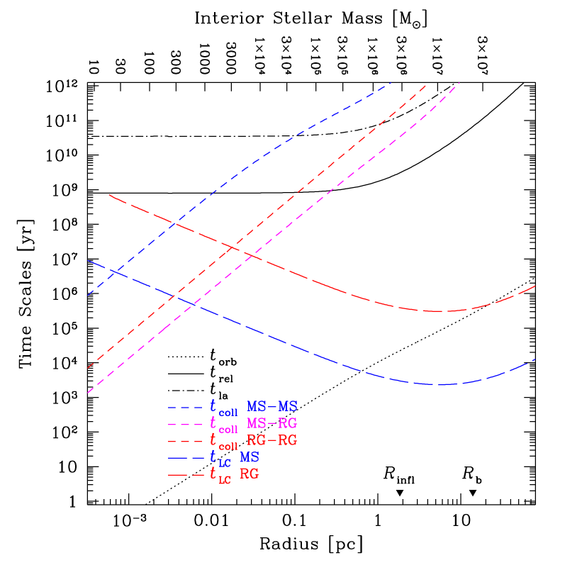
Figure 3.— Time scales in our reference model of the MW nucleus ($M_{\rm cl}={7}\times 10^{7}\,{\rm M}_{\odot}$, $\eta=1.5$, $R_{\rm NB}=28\,$pc). We plot the orbital time $t_{\rm orb}$ (assuming a circular orbit), the relaxation time $t_{\rm rlx}$, the time scale for large-angle deflections $t_{\rm la}$, collision times $t_{\rm coll}$ and the timescale for diffusion by 2-body relaxation over the loss cone for tidal disruption, $t_{\rm LC}=\theta_{\rm LC}^{2}t_{\rm rlx}$. For collisions we indicate the average time for a MS star to collide with another MS star or with a red giant (RG) and the average time for a RG to collide with another RG. We assume $M_{\rm MS}=M_{\rm RG}=1\,{\rm M}_{\odot}$, $R_{\rm MS}=1\,{\rm R}_{\odot}$, $R_{\rm RG}=50\,{\rm M}_{\odot}$, and 5 % of RGs. The radius where $t_{\rm orb}=t_{\rm LC}$ is the critical radius.

There are only few published models for (spherical) clusters in dynamical equilibrium and containing a massive central object. The best described and most convenient ones are the “eta-models” introduced by Dehnen (1993) and extended to systems with a central object by Tremaine et al. (1994). The density profile is

$$\rho(R)=\frac{\eta M_{\rm cl}}{4\pi R_{\rm b}^{3}}\left(\frac{R}{R_{\rm b}}\right)^{\eta-3}\left(1+\frac{R}{R_{\rm b}}\right)^{-\eta-1}.$$ (13)

The exponent $\eta$ can take any value between 0 and 5/2. At small radii, $\rho\propto R^{-\gamma}$ with $\gamma\equiv 3-\eta$ while at large distances, density falls off like $R^{-4}$. The break radius can easily be expressed in terms of other important length scales,

$$R_{\rm b}=(2\eta-1)^{-1}R_{\rm NB}=(2^{1/\eta}-1)R_{\rm h}.$$ (14)

The fraction of the stellar mass enclosed by $R_{\rm b}$ is $2^{-\eta}$. The central MBH defines a second dimensionless parameter $\mu\equiv M_{\bullet}/M_{\rm cl}$.

At short distances from it, the MBH dominates the dynamics and therefore $\sigma^{2}(R)\approx\sigma^{2}_{\rm MBH}(R)=(4-\eta)^{-1}GM_{\bullet}/R$. We define the influence radius $R_{\rm infl}$ implicitly through $\sigma^{2}(R_{\rm infl})=2\sigma^{2}_{\rm MBH}(R_{\rm infl})$. Figure 1 shows how $R_{\rm infl}$ depends on $\mu$ for various values of $\eta$. In the present study, we use eta-models as a way to carry out simulations with a power-law density cusp of controlled exponent $\gamma$ as initial conditions. We view the steeper density decrease at large radii, $R>R_{\rm b}$, as a cut-off to avoid wasting computer memory and CPU time by putting a large number of particles at distances that should not be influenced by the presence of the MBH through relaxation effects. In other words, the value of $R_{\rm b}$ should be irrelevant as long as it is large enough to encompass the region within which the collisional physics takes place. It is therefore important to have $R_{\rm b}>R_{\rm infl}$ and, from Figure 1, we see that this will be the case for $\eta=1-2.25$ provided that $\mu\leq 0.05$. For $\eta\leq 1.5$, $\mu\leq 0.1$ should be sufficient.

Another important radius is the critical radius for tidal disruptions, $R_{\rm cr,td}$ (Frank & Rees 1976; Lightman & Shapiro 1977; Magorrian & Tremaine 1999; Syer & Ulmer 1999; Amaro-Seoane et al. 2004). It is defined as the position in the cluster where the diffusion angle caused by relaxation per orbital time equals the opening angle of the loss cone, for a typical MS star,

$$\left(\frac{\pi}{2}\right)^{2}\frac{P_{\rm orb}}{t_{\rm rlx}}=\theta_{\rm LC}^{2}.$$ (15)

A local, typical value of $\theta_{\rm LC}$ can be obtained by computing it for a star whose velocity would be equal to the (3D) velocity dispersion, i.e., solving Eq. 23 of Freitag & Benz (2002b) with $v^{2}=3\sigma^{2}(R)$.

The rate of tidal disruptions is dominated by the contribution of stars with apocenter distances of order of the minimum between $R_{\rm infl}$ and $R_{\rm cr,td}$. For all models considered in this study, $R_{\rm cr,td}<R_{\rm infl}<R_{\rm b}$ (see Figure 3) so the loss-cone effects should be little affected by the existence of a steeper density decrease beyond $R_{\rm b}$.

For the present study we construct most models so that they best approximate the conditions in the MW nucleus. In Figure 2, we plot the enclosed mass as a function of radius for some of our initial models and compare with observational data (Schödel et al. 2003; Ghez et al. 2005). Our reference cluster model is described by $M_{\bullet}={3.5}\times 10^{6}\,{\rm M}_{\odot}$, $M_{\rm cl}={7}\times 10^{7}\,{\rm M}_{\odot}$ (hence $\mu=0.05$), $\eta=1.5$ and $R_{\rm NB}=28\,$pc. This model has a central density cusp with $\gamma=1.5$, a value consistent with the stellar counts at the galactic center (Alexander 1999; Genzel et al. 2003). However, a detailed modeling of the Galactic center is not our goal. This would in particular require ad hoc assumptions regarding the history and locations of star formation to account for a population with a variety of ages (Figer et al. 2004). This variety could be the result of the intermittent formation, at a few pc from the center, of small clusters that then spiral in and deposit their stars in the nucleus (see, e.g., Maillard et al. 2004; Paumard et al. 2004; Lu et al. 2005 for observations and Kim & Morris 2003; Portegies Zwart et al. 2003; Kim et al. 2004; Gürkan & Rasio 2005 for simulations).

Separate from the MW-like models, we explore the effects of mass segregation in idealized galactic nucleus models with a variety of structural parameters. We consider nuclei with $M_{\bullet}$ in the range $10^{5}-10^{7}\,{\rm M}_{\odot}$. To decrease the dimensionality of the parameter space, we assume the $M-\sigma$ relation (Merritt & Ferrarese 2001; Tremaine et al. 2002; Barth et al. 2005) to hold perfectly,

$$M_{\bullet}\simeq M_{100}\left(\frac{\sigma}{100\,\mathrm{km\,s}^{-1}}\right)^{\beta}.$$ (16)

Tremaine et al. (2002) find $\beta=4.0\pm 0.3$ and $M_{100}={8.3^{+5.5}_{-3.3}}\times 10^{6}\,{\rm M}_{\odot}$. With a velocity dispersion of $\sigma\simeq 100\,\mathrm{km\,s}^{-1}$, the MW harbors an under-massive MBH. We note, however, that the velocity dispersion of the MW central region, as defined for use in Eq. 16, is dominated by stars located at a few hundreds pc from the center (Tremaine et al. 2002, and references therein), a region we do not attempt to model. The MW nucleus is the only one whose structure is relatively well constrained by observations at the scales of interest here ($R<10\,$pc). Hence, for simplicity we adopt the MW nucleus as typical. A model for a nucleus with an MBH of mass $M_{\bullet}$ is obtained from a MW model of same $\eta$ and $\mu$ by simple length (and mass) rescaling. As $R\propto M\sigma^{-2}$ and using $\beta=4$ we obtain:

$$R_{\rm NB}=\left.R_{\rm NB}\right|_{\rm MW}\left(\frac{M_{\bullet}}{{3.5}\times 10^{6}\,{\rm M}_{\odot}}\right)^{1/2}$$ (17)

where $\left.R_{\rm NB}\right|_{\rm MW}$ is the $N-$body radius of the MW model. Neglecting the dependence of the Coulomb logarithm on $N_{\ast}$, the relaxation time of the model scales like $t_{\rm rlx}=\left.t_{\rm rlx}\right|_{\rm MW}({M_{\bullet}}/{{3.5}\times 10^{6}\,{\rm M}_{\odot}})^{5/4}$. It follows that $t_{\rm rlx}(R_{\rm infl})$ exceeds $\sim 10$ Gyr for $M_{\bullet}\gtrsim 10^{7}\,{\rm M}_{\odot}$ and we expect only minor relaxation effects in such massive nuclei. The lowest MBH mass we consider, $10^{5}\,{\rm M}_{\odot}$, corresponds to that of the smallest MBH detected with some confidence in a galactic center so far (Barth et al. 2004, 2005). Even smaller systems, such as the nuclei of dwarf galaxies or globular clusters may host intermediate mass black holes (IMBHs) with $M_{\bullet}<10^{5}\,{\rm M}_{\odot}$. We do not address the evolution of low-mass objects here because their central dynamics may be significantly influenced by small-$N_{\ast}$ effects not included in ME(SSY)$\ast\ast$2. Recently, the very significant increase of computational power offered by special-purpose GRAPE hardware (Makino et al. 2003), combined with a variety of mathematical and numerical techniques to speed up computations (Aarseth 2003) have made it possible to follow the relaxation evolution of clusters with a central massive object and up to ${2.5}\times 10^{5}$ stars by “direct” $N-$body integrations (Baumgardt et al. 2004a, b, 2005; Preto et al. 2004). However, because of the steep dependence of the CPU time on the number of particles imposed by direct force computations in the $N-$body algorithm (approximately $T_{\rm cpu}\propto N_{\rm p}^{3}$ per relaxation time), systems containing $\sim 10^{6}$ stars or more can only be studied with more approximate methods such as MC codes.

The range $M_{\bullet}=10^{5}-10^{7}\,{\rm M}_{\odot}$ also corresponds to the MBH around which an EMRI has the best chance to be detected by LISA. The orbital period of a test particle on the innermost stable circular orbit around a non-rotating BH of mass $M_{\bullet}$ is

$$f_{\rm ISCO}\simeq\frac{c^{3}}{2\pi 6^{3/2}GM_{\bullet}}={2.2}\times 10^{-3}\,{\rm Hz}\left(\frac{M_{\bullet}}{10^{6}\,{\rm M}_{\odot}}\right)^{-1}.$$ (18)

Consequently, inspirals into MBH more massive than $\sim 10^{7}\,{\rm M}_{\odot}$ produce signals with frequency too low for LISA to detect, while the final inspiral into an MBH with $M_{\bullet}\lesssim 10^{5}\,{\rm M}_{\odot}$ occurs at periods higher than the time taken by light to travel along LISA arms, which strongly reduces sensitivity at those frequencies (Larson et al. 2000). In principle EMRIs into such lower-mass MBH could be caught at an earlier phase in their orbital evolution but the emitted waves have much lower amplitude then, thus severely limiting the detection range (Will 2004). Furthermore, the analysis of Hopman & Alexander (2005) indicates that most stellar objects closely bound to an IMBH will be scattered on to a direct plunge orbit before they enter the LISA band. These authors predict that successful (i.e. gradual) LISA inspirals around IMBH have to start at very high eccentricities and small semi-major axis and should last only $\sim 1$ year before coalescence.

In this study, we concern ourselves with the idealized situation of an isolated, gas-free galactic nucleus. In particular, we do not consider the effects of interactions with other galaxies, such as mergers with other nuclei or gas inflow. Similarly, we neglect the possibility of smaller stellar clusters spiraling down to the galactic center or non-spherical mass distributions. Finally, we assume that all stars have formed in a single burst with no further star formation. For the models in which stellar evolution or collisions are included, the gas lost by stars is considered instantaneously lost from the system, with, in some cases, a fraction being accreted by the central MBH.

Some of these simplifications, most noticeably that of spherical symmetry and absence of gas, are required by the numerical methods used. Others are made in order to reduce the complexity of the problem and the dimensionality of the parameter-space, hence allowing a better understanding of the systems under study.

Most of our simplifying assumptions favor mass segregation of stellar BHs, our primary object of study. For instance, it seems likely that a merger between nuclei induces violent relaxation, thus erasing –at least partially– any previous mass segregation. If both nuclei contain a MBH, the binary MBH will eject stars from the central regions and strongly decrease the density there, thus lengthening relaxation time (e.g., Milosavljević & Merritt 2001; Makino & Funato 2004). Also, if stars are formed over an extended period of time instead of all being born at some “initial” time, stellar BHs will, on average, have less time to experience mass segregation.

Cosmological simulations indicate that most normal galaxies have not suffered a major merger for several Gyrs. In particular, some 5-7 Gyr are probably required for a disk to (re)form after a merger (Governato et al. 1994; Abadi et al. 2003). Therefore our simulations can be considered to cover the evolution of a galactic nucleus since it experienced its last major merger. We will focus our analysis on the structure of the nucleus after 5 and 10 Gyr of simulated evolution; 5 Gyr is a reasonable value for the period of time during which a nucleus in the present-day universe may have evolved without strong interactions; 10 Gyr is an upper limit that enables us to see what the maximum effects of relaxation are likely to be. Mergers probably lead to important gas inflow into the central regions, triggering stellar formation and accretion onto the MBH, in a complex interplay (e.g., Springel et al. 2005). In such episodes the MBH may grow substantially on time scales shorter than the relaxation time, but still significantly longer than stellar orbital periods. The stellar nucleus then contracts adiabatically in response to the deepening of the MBH potential (Young 1980; Quinlan et al. 1995; Freitag & Benz 2002b). To investigate the impact of such episodes on the structure of the nucleus several Gyrs later, and contrast it with our standard models where the mass of the MBH increases only little during the course of the simulation (by tidally disrupting and capturing stars), we computed a few models in which a central BH of small mass ($\mu(t=0)=10^{-5}$) grows rapidly by accreting some fraction of the gas released due to stellar evolution.

3.3. Stellar Population and Evolution

Except for a few test-case models presented in § 4.1, we use the “Kroupa” initial mass function (IMF) for all our models (Kroupa et al. 1993; Kroupa 2001a, b). It is a broken power-law, $dN_{\ast}/dm_{\ast}\propto m_{\ast}^{-\alpha}$, with $\alpha=0.3$, $1.3$ and $2.3$ in the ranges $m_{\ast}/{\rm M}_{\odot}\in[0.01,0.08[$, $[0.08,0.5[$ and $[0.5,120]$, respectively. We generally consider the range $0.2-120\,{\rm M}_{\odot}$ for stellar masses on the MS.

In most simulations, we do not include stellar evolution but start with a stellar population in which all stars already have an age of 10 Gyr. This is of course not a physically consistent treatment but we choose it for the sake of simplicity. For comparison purposes, in a few simulations, stellar evolution is included and those simulations are started with zero-age MS stars. The main impact of stellar evolution is to induce significant mass loss in the first $\sim 10^{8}$ years. As we will see, the nucleus experiences strong expansion if this gas is expelled from it. To produce such a model for a nucleus with specific current properties (as those of the MW), we have to find, by trial-and-error, initial cluster structural parameters leading, after $5-10$ Gyr, to a nucleus model fitting the observations (in our case, the enclosed mass as function of radius).

We use a simple stellar evolution prescription according to which stars keep a fixed mass and radius while on the MS and instantaneously turn into compact remnants (CRs) at the end of their MS lifetime, $t_{\rm MS}(m_{\ast})$. Data for $t_{\rm MS}(m_{\ast})$ were provided by K. Belczynski (Hurley et al. 2000; Belczynski et al. 2002). As for the relation between the stellar mass on the MS and the nature and mass of the CR, we consider three models, presented in Table 1. In the first one, dubbed “fiducial” (F), we assume all white dwarfs (WDs), neutron stars (NSs) and stellar BHs have a mass of $0.6$, $1.4$ and $10\,{\rm M}_{\odot}$ respectively. The two other models make use of the prescriptions developed by Belczynski et al. (2002), assuming either solar ($Z=0.02$, model “BS”) or metal-poor ($Z=10^{-4}$, model BP) chemical composition. These prescriptions represent our current understanding (although incomplete) of massive-star core collapse and possible fallback onto the nascent compact remnant. The quantitative aspects are consistent with the hydrodynamic calculations presented in Fryer (1999) and the resulting relations between MS and CR masses are shown in Figure 1 of Belczynski et al. (2002). When stellar evolution is included, we impose that the time step is smaller than a factor $f_{\rm SE}$ times the MS life time $t_{\rm MS}$ for all stars still on the MS. We have set $f_{\rm SE}=0.1$ after have checked that results are essentially the same as with $f_{\rm SE}=0.025$.

To explore the effect of supernova kicks in some simulations with stellar evolution, we give NSs and BHs a velocity kick at birth. Although the mechanism responsible for such “natal kicks” is still not understood, they are required to explain the high spacial velocities of observed field pulsars (Hobbs et al. 2005, and references therein) as well as other observed characteristics of neutron star binaries (e.g., Willems et al. 2004; Thorsett et al. 2005, and references therein).

There are also observations and interpretation analyses suggesting that some BHs receive a kick at birth (Mirabel et al. 2001, 2002; Gualandris et al. 2005a; Willems et al. 2005). It is generally accepted that a supernova explosion is required to provide the natal kick. Consequently, it is likely that only BHs formed through the fallback mechanism, with a progenitor less massive than $m_{\rm FB}\approx 42\,{\rm M}_{\odot}$ receive kicks (Fryer & Kalogera 2001; Heger et al. 2003). In the MC simulations with natal kicks, we base our prescription on the results of Hobbs et al. (2005). The kick velocity is picked from a single Maxwellian distribution with a one-dimensional dispersion of $\sigma_{\rm NK}=265(1.4\,{\rm M}_{\odot}/m)\,\mathrm{km\,s}^{-1}$ where $m$ is the mass of the NS or BH. BHs resulting from the evolution of a MS star more massive than $42\,{\rm M}_{\odot}$ are not given any kick.

4. Results of Simulations

Our simulations fall into two categories. First are a few cases with a single-mass or a two-component stellar population. They are used to test the MC algorithm by comparison with analytical or $N-$body results. The second category consists of more than 80 galactic nucleus models with more realistic choices of parameters and stellar populations. In what follows we describe the results of some representative runs and explain how the important outcomes are affected by the initial conditions and physics.

4.1. Test Models

Figure 4.— Evolution of the density profile for a single-mass cluster with $\eta=2.25$ and $\mu=M_{\bullet}/M_{\rm cl}=0.05$ simulated with 4 million particles. Note the establishment of a $\rho\propto R^{-1.75}$ cusp and the expansion of the cluster, driven by diffusion of stars towards the MBH.

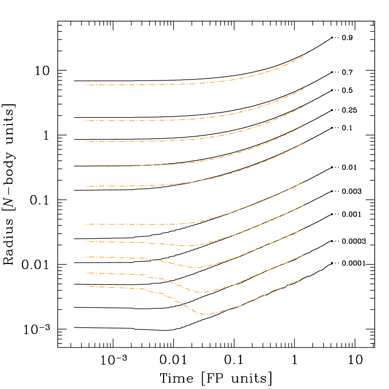
Figure 5.— Comparative evolution of single-mass models with different initial central density profiles. We plot the Lagrange radii, i.e. the radius of spheres enclosing the indicated fraction of the total stellar mass. Models with $\eta=1.5$ (solid lines) and $\eta=2.25$ (dash-dot) are compared. Both runs have $\mu=0.05$ and $N_{\rm p}={4}\times 10^{6}$. At late times, the two cases have converged to the same structure and evolution.

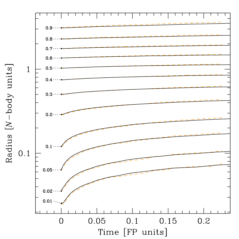
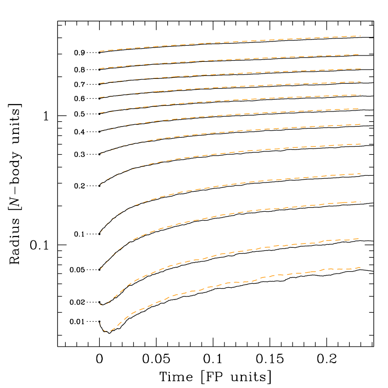
Figure 6.— Comparison of the Lagrange radii evolution between $N-$body results from Baumgardt et al. (2004a) and our ME(SSY)$\ast\ast$2 simulations of single-mass cluster models. From top to bottom, the panels correspond to models 1, 2 and 4 in Table 1 of Baumgardt et al. (2004a). The MC results are plotted with solid lines, the $N-$body results with dashed lines. We present MC results obtained with $N_{\rm p}=N_{\ast}=80\,000$ for case 1 and 4 (top and bottom) and $N_{\rm p}=5\,N_{\ast}=320\,000$ for case 2. A run with $N_{\rm p}=N_{\ast}=80\,000$ gives very similar (but noisier) results. The $N-$body time unit is converted into FP unit assuming $\gamma_{\rm c}=0.11$. The curves have been smoothed with a running averaging procedure using a Gaussian Kernel.

Since ME(SSY)$\ast\ast$2 was originally developed and tested (Freitag & Benz 2001, 2002b), the code has gone through many small revisions. Furthermore, at that time, only few direct $N-$body simulations had been published with high enough resolution to yield test cases to which the results of the more approximate MC code could be usefully compared. The advent and spectacular increase of computing speed of GRAPE boards now permits more comparisons, although restrictions in the applicability of comparisons still exist. We have recently carried out new tests for the core-collapse evolution of clusters with a variety of stellar mass functions but no central object (Freitag et al. 2006). Here, we investigate models with a central MBH. We compare MC results with simple semi analytical predictions as well as published and original $N-$body simulations, presented here for the first time.

The development of a $\rho\propto R^{-1.75}$ density cusp in a single-mass cluster hosting a central MBH has been a well-accepted theoretical prediction for nearly 30 years (Bahcall & Wolf 1976), but has only recently been verified by direct $N-$body simulations (Preto et al. 2004; Baumgardt et al. 2004a). In Figure 4 we show how such a profile forms in one of our single-mass MC simulations of a cluster model with $\eta=2.25$, $\mu=0.05$ and $N_{\rm p}={4}\times 10^{6}$. It is evident that at late times, the evolution is an approximately self-similar expansion of the cluster, driven by destruction of stars by the MBH (whose mass was kept constant in this simulation). Models with different initial $\eta$ values converge to the same structure and evolution after $t\approx(0.05-0.1)\,T_{\rm FP}$, as illustrated in Figure 5. To measure the speed at which the central regions evolve, the relaxation time at the influence radius, $t_{\rm rlx}(R_{\rm infl})$ (using Eq. 2.1), is a more relevant timescale than $T_{\rm FP}$; we find $t_{\rm rlx}(R_{\rm infl})={2.2}\times 10^{-3}\,T_{\rm FP}$ for $\mu=0.05$, $\eta=1.5$ and $t_{\rm rlx}(R_{\rm infl})={4.9}\times 10^{-3}\,T_{\rm FP}$ for $\eta=2.25$. Hence, the full development of a Bahcall-Wolf cusp requires of order $10\,t_{\rm rlx}(R_{\rm infl})$ in a single-mass cluster.

With an $N-$body code, Baumgardt et al. (2004a) have computed the evolution of single-mass $W_{0}=10$ King models (Binney & Tremaine 1987; Heggie & Hut 2003) with a central BH of $\mu$ in the range $0.0026-0.1$ (the stellar velocities were modified to ensure approximate dynamical equilibrium). The central BH was allowed to grow in mass by disrupting stars at $R_{\rm t.d.}=(10^{-9}-10^{-7})R_{\rm NB}$ and fully accreting their mass. As Figure 6 clearly indicates, we can reproduce the evolution of such systems in a satisfactory manner using ME(SSY)$\ast\ast$2. We have also checked that our results are insensitive to the particle number (as long as it is large enough) by repeating a few models with $N_{\rm p}=5N_{\ast}$ instead of $N_{\rm p}=N_{\ast}$. On the other hand, we have found the MC results to be more sensitive on the time step parameter than one might hope. For these single-mass models, $f_{\rm\delta t}=0.005-0.01$ gives the best results (see Freitag & Benz 2001 for an explanation of how the time steps are determined in ME(SSY)$\ast\ast$2; in rough terms $f_{\rm\delta t}$ is a prescribed upper bound on $\delta t(R)/t_{\rm rlx}(R)$). With larger values, the deflection angles in “super-encounters” become too large, leading to too little relaxation (and hence evolution) per unit of simulated physical time.

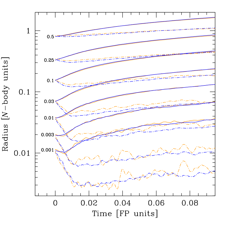
Figure 7.— Comparison between our Nbody4 and ME(SSY)$\ast\ast$2 simulations of a 2-component cluster model. The evolution of Lagrange radii for the indicated mass fractions of each component is plotted. The initial structure is an $\eta-$model with $\eta=2$ and $\mu=0.1$. The population consists of light stars with $m_{\rm light}=1\,{\rm M}_{\odot}$, shown with solid lines, and of 5 % (in number) of heavy objects with $m_{\rm heavy}=10\,{\rm M}_{\odot}$, shown with dash-dotted lines. For these runs both types are treated as MS stars, subject to tidal disruption by the central BH. The physical scales are set by $R_{\rm NB}=1\,\mathrm{pc}$ and $N_{\ast}=64\,000$. The gray (orange) curves show the results of the $N-$body simulation, realized with $N_{\rm p}=64\,000$. The black curves are for the MC run which used $N_{\rm p}=640\,000$. The $N-$body time unit is converted into FP unit assuming $\gamma_{\rm c}=0.02$. The Lagrange radii for the $N-$body run are determined, at each snapshot, through a procedure of “orbital oversampling” in which the position of each particle on its orbit is sampled many times, with probability density $dP/dR\propto v_{r}^{-1}(R)$, assuming a spherically symmetric potential centered on the IMBH. This way, one can follow a fractional mass as low as 0.001 which represents only 3.2 particles for the heavy stars.

Figure 8.— Comparison of the density profiles between our Nbody4 and ME(SSY)$\ast\ast$2 simulations of a 2-component cluster model. Thick solid and dash-dotted lines show the mass density for light stars (“MS”) and massive ones (“BH”), respectively; the thin lines are the total densities. The $N-$body and MC results are shown in gray and black, respectively. We also add straight lines representing power laws with $\gamma=1.75$ and $\gamma=1.5$.

The next step is to consider 2-component models in which a small fraction $f_{\rm heavy}$ of the stars are significantly more massive than the rest with $q=m_{\rm heavy}/m_{\rm light}\geq 10$. However, there are no published results of this type using N-body simulations that can provide a well-controlled test case. For this reason we have undertaken our own $N-$body simulations using Nbody4, a code developed and made freely available by Sverre Aarseth. Modifications were made to the code to include tidal disruptions and BH mergers. Over the years, Aarseth’s Nbody family of codes have become central workhorses in a great number of stellar dynamical projects. They are described in detail in Aarseth (1999, 2003). Nbody4 can exploit a GRAPE board to accelerate the computation by a very large factor (Makino et al. 2003), which proved essential to obtain the results presented here.

To represent stellar BHs in a population of age 5–10 Gyr $q\simeq 20-40$ and $f_{\rm heavy}\simeq{(1-3)}\times 10^{-3}$ would be adequate but such small fractions cannot be adopted usefully in $N-$body simulations with $N_{\rm p}\lesssim{1.3}\times 10^{5}$, the highest number of particles that can be used on the micro-GRAPE hardware at our disposal. To have a reasonably large number of heavy particles, we have chosen $f_{\rm heavy}=0.05$ and $q=10$ for a simulation with $N_{\rm p}=64\,000$. The initial structure of the cluster is an $\eta-$model with $\eta=2$ and $\mu=0.1$. For simplicity, we have assumed that all stars have a MS size and are tidally disrupted if they come within $R_{\rm t.d.}$ of the IMBH, itself treated as a massive particle (rather than an external potential). When a star is tidally disrupted its whole mass is given to the IMBH. The size is set to $R_{\rm NB}=1\,\mathrm{pc}$. MC models were run with $N_{\rm p}=N_{\ast}$ (“64k”), $N_{\rm p}=5N_{\ast}$ (“320k”) and $N_{\rm p}=10\,N_{\ast}$ (“640k”) for higher resolution and to permit a better determination of the local density, particularly near the cluster center, as needed by the MC algorithm for robust results. Actually, the results turn out to depend very little on $N_{\rm p}$..

Figure 7 offers a global view on how the spatial distributions of light and heavy particles evolve with time in the $N-$body and MC simulations. For the $N-$body simulation, the center of the system, from which distances are measured, was defined to be the (instantaneous) position of the IMBH. As the natural time scale is dynamical for the $N-$body code ($T_{\rm NB}$) but relaxational for the MC algorithm ($T_{\rm FP}$), one needs to specify $\gamma_{\rm c}$ to compare the results in the same time units. We find the best agreement with $\gamma_{\rm c}=0.01-0.02$, as was the case for the (I)MBH-less multi-mass systems simulated by Freitag et al. (2006). For the light particles, the concordance between the methods is excellent. The heavy particles, on the other hand, show some discrepancy. The MC code produces mass segregation at a rate almost equal to that seen in the N-body runs. The heavy objects appear to concentrate slightly more at the center before the whole cluster starts expanding slowly.

The nature of the difference between the results from the two codes is seen more clearly in Figure 8 where a snapshot of the central density profiles at nearly the same time is shown. The MC run shows a Bahcall-Wolf cusp of BHs that extends all the way down to the resolution limit. In contrast, the $N-$body profile appears to flatten slightly inside $R\approx 0.01\,R_{\rm NB}$. Given that the region with this flattened profile involves only $5-10$ BH particles at a time in the $N-$body simulation, this mismatch could be deemed of little significance, if it were not consistently present in most snapshots. We have redone the MC simulations with or without large-angle scatterings or tidal disruptions of the MS stars and found that the results are not altered: in all cases, the BHs develop a slightly more pronounced innermost density peak than in the $N-$body run. The fact that in the MC simulation the central BH is assumed to be fixed in position may be the cause of the difference; this is supported by the amplitude of the IMBH wandering in the $N-$body run, $\sim 0.01\,R_{\rm NB}$ (comparable to the spatial extent of the flattened profile). If this is the case, the effect should be less important in galactic nuclei, as far as the distribution of stars around the MBH is concerned because the wandering –essentially the manifestation of energy equipartition– decreases with decreasing mass ratio $m_{\ast}/M_{\bullet}$ (Laun & Merritt 2004, and references therein). In our $N-$body simulation, this ratio is is $\sim 10^{-4}$ and $\sim 10^{-3}$ for light and heavy stars respectively. In a galactic nucleus with a $10^{6}\,{\rm M}_{\odot}$ MBH, the ratio is $10^{-5}$ at most.

Last we examine the density profiles shown in Figure 8. Specifically those obtained with the MC code (less affected by small-number effects) clearly indicate that the light objects follow a profile compatible with $\gamma=1.5$ only at distances smaller than $R_{1.5}\approx 0.01\,R_{\rm NB}$, whereas the radius encompassing a mass of stars equivalent to $M_{\bullet}$ (an approximation to $R_{\rm infl}$) is of order $0.2-0.3\,R_{\rm NB}$. Only within $R_{1.5}$ is the number space density of stars dominated by BHs. Between $R_{0.5}$ and $R_{\rm infl}$ is a transition region in which $\gamma<1.5$ for the light objects even though $\gamma\simeq 1.75$ for the heavy ones. Similar findings were obtained by Baumgardt et al. (2004b). Although these results do not invalidate the prediction from the Fokker-Planck treatment that light objects should form a cusp with $\gamma=1.5$ close to the central (I)MBH (Bahcall & Wolf 1977; Gnedin & Primack 2004), they indicate that, unless the fractional number of massive objects is unrealistically high (as is the case in the test-computation presented by Murphy et al. 1991 in their Figure 9), this regime may only be attained in a very small central volume and therefore will be of relatively little relevance to real systems.

4.2. Realistic Models

4.2.1 Sgr A^∗-type models

Figure 9.— Evolution of Lagrange radii for a “standard” MW nucleus model GN25. We plot the evolution of the radii of spheres that enclose the indicated fractions of the mass of various stellar species. Solid lines are for MS stars, short-dashed lines for white dwarfs, long-dashed lines for neutron stars and dash-dotted lines for stellar BHs.

Figure 10.— Evolution of the density profiles for a “standard” MW nucleus model GN25 (same model as Figure 9). On the last panel, we indicate the power-laws that appear consistent (visually) with the central density profiles of the MS stars and stellar BHs. The BH exponent, $\gamma\simeq 1.8$ is very close to $\gamma=1.75$ predicted by Bahcall & Wolf (1976, 1977) but the lighter objects form a cusp shallower than $\gamma=1.5$ (see discussion in text).

Figure 11.— Evolution of the profiles of enclosed mass for GN25. The solid lines are the results of the MC simulation. For reference, he dashed lines show $\eta=1.5$ profiles adjusted on the total mass and half-mass radius of each component. The top thin line is the total mass, including the central MBH; it is compared to the observational constrains for the MW center (see Figure 2).

Figure 12.— Evolution of Lagrange radii for a nucleus model without stellar BHs (GN49).

Figure 13.— Differential mass segregation amongst MS stars. For model GN44, in which the IMF extends down to $0.01\,{\rm M}_{\odot}$ (instead of being truncated at $0.08\,{\rm M}_{\odot}$), we plot the evolution of Lagrange radii for MS stars in three different mass bins. The lightest objects expand only slightly more than the most massive ones. For each bin, we indicate the average mass $\langle m_{\ast}\rangle$ and mass fraction $\rm f_{\rm m}$.

Figure 14.— Comparison of the evolution of two nucleus models with similar initial conditions but different values of $\eta$: $\eta=2.25$ (GN20; top panel) and $\eta=1.5$ (GN17; bottom panel). Note that the conversion factors between $N-$body and FP units (for length and time, respectively) and physical ones are different in each case.

Next we consider models specifically intended to represent galactic nuclei. The parameters describing the initial conditions for these simulations are listed in Table 2.

Let us first consider in some detail the evolution of our “standard model”, run GN25 with $\eta=1.5$ and $\mu=0.05$. These parameters are adapted to fit the observed enclosed mass profile of the MW center (Schödel et al. 2003; Ghez et al. 2005). The physics implemented in this model is limited to 2-body relaxation, tidal disruptions of stars by the central MBH (which accretes 50 % of the stellar mass) and direct plunges through the horizon. We use stellar population F. This is one of the highest resolution models with $N_{\rm p}={8}\times 10^{6}$ and each particle representing $26.65$ stars (note that the MC code does not require a particle to stand for an integer number of stars).

The overall evolution of the nucleus structure is depicted in three different (but essentially equivalent) ways in Figures 9, 10 and 11. In Figure 9 we present a general overview by showing how the Lagrange radii of the various stellar types evolve with time. The development of mass segregation is clearly apparent. Qualitatively, the region of influence of the MBH corresponds to the extent of the MS Lagrange radius for a fractional mass equal to the value of $\mu=M_{\bullet}/M_{\rm cl}$, i.e. 0.05. Deep in this region, the evolution is approximately homologous. The stellar BHs concentrate in the center over a timescale $\sim{(1-2)}\times 10^{-3}\,T_{\rm FP}\approx 4-8\,$Gyr. At the same time, the other stars slightly expand out of the center but the total density profile stays nearly constant.

During this first phase, the BHs come to dominate the central mass density by forming a cusp around the MBH. This can be seen in Figure 10. We note that, at late times, the cusp exponent becomes compatible with $\gamma=1.75$, but the lighter objects form a profile with $\gamma<1.5$, flatter than the Bahcall & Wolf (1977) exponent. However, it must be stressed that, for this model, the stellar BHs never contribute more than $\sim 15$ % of the number density in any region. Therefore they do not become a strictly dominant species, in the sense that they still experience most of their interactions with lighter objects. This is different from the situation studied by Bahcall & Wolf (1977), who only considered larger values for the number fraction $f_{\rm heavy}$ of massive objects (their smaller value being $f_{\rm heavy}=1/16$ while we have $f_{\rm heavy}=f_{\rm BH}\simeq 0.002$) and smaller mass ratios $q=m_{\rm heavy}/m_{\rm light}$ (they have $q\leq 10$ while we have $q\approx 20-30$). Because our particle number is not large enough to treat the system on a star-by-star basis, it is still possible that, in a real MW-like nucleus, there would be a region very close to the central MBH in which the stellar BHs are numerically dominant and a clean Bahcall & Wolf (1977) cusp could form. Our results strongly suggest that the radius of this region is at least 100 times smaller than $R_{\rm infl}$.

All other stellar species react to the segregation of the stellar BHs by expanding away from the center. This evolution is very similar for all objects of mass significantly lower than that of the BHs, with the NSs showing slightly less expansion than the MS and WD stars. However, to the resolution limit of our simulations, the density profiles show no conspicuous central depletion, such as a flattening or even a dip (as suggested by Chanamé & Gould 2002 for pulsars around Sgr A^∗). Such a density decrease is apparent only in comparison with the initial conditions. It is very unlikely that this density decrease can be revealed by observations in the Galactic center as a tell-tale indication of the presence of a cusp of stellar BHs. Also, MS stars of different masses react essentially the same way, as can be seen in Figure 13, and end up having the same density profiles.

The fact that the stellar BH population is the main driving cause for the evolution of the central parts of our nucleus models becomes clear by running a simulation without any BHs (see Figure 12). The most obvious difference is that the overall evolution, now driven by the mass segregation of NSs, is of order $5-10$ times slower, reflecting a correspondingly longer dynamical-friction time scale. The NSs are fully segregated only after of order 30–40 Gyr. Consequently, even a clear-cut observation that old visible stars form a $\gamma\lesssim 1.5$ at the center of the MW could not be interpreted as (indirect) evidence for the existence of a population of invisible BHs following a steeper profile: if BHs are not present, the system evolves too slowly to reach a relaxed state over 5–10 Gyr and the observed distribution may still reflect some “initial conditions” impose, for example, by a merger with another nucleus or by a large starburst due to massive gas inflow.

We note that the choice of $\eta=1.5$ as initial condition is rather arbitrary. It is mostly motivated by the observational constrains on the present-day stellar distribution around Sgr A^∗. We have considered models with $\eta$ in the range $1.2$ ($\gamma=1.8$) to $2.25$ ($\gamma=0.75$) to assess the importance of the initial density profile on the late-time structure and evolution of our models. In Figure 14, we compare the evolution of two models that share the same physics and most initial conditions, including the total mass, the mass of the MBH, the stellar population and (approximately) the enclosed stellar mass within 1 pc, but different central profiles, namely $\eta=2.25$, corresponding to a shallow cusp, and our usual $\eta=1.5$. The $\eta=2.25$ model shows more evolution in the first $6-8$ Gyr as it “catches up” with the $\eta=1.5$ case. After $t\sim 8$ Gyr, however, both nuclei have similar structures. In both cases, the BHs dominate the mass density inside $R\simeq 0.3\,\mathrm{pc}$ (where their density is $\simeq{2}\times 10^{5}M_{\odot}\,\mathrm{pc}^{-3}$) at $t\simeq 10$ Gyr. At that time, the BHs and MS stars form cusps with $\gamma=1.7-1.8$ and $\gamma=1.3-1.4$, respectively (for $R\lesssim 0.15\,\mathrm{pc}$) for both simulations. In other terms, in the region of influence of the MBH, a period of time of order $t_{\rm rlx}(R_{\rm infl})$ (which translates into $7-10$ Gyr for our MW-like models) seems enough to erase the details of the “initial conditions”.

Figure 15.— Number of stars of different types within $0.1$, $0.3$ and $1\,\mathrm{pc}$ from the center for model GN25. Solid lines indicate MS stars, short dashes WDs, long dashes NSs and dash-dotted lines stellar BHs. The dotted lines are the result of the application of the analytical formula for dynamical friction (equations 8 and 9) for the BHs, assuming a static background defined by the $\eta$-model and average stellar mass of the initial conditions. BHs that would have reached $R=0$ by dynamical friction are considered accreted by the MBH and not counted.

The initial conditions of model GN25 were chosen to be compatible with the overall mass distribution in the Sgr A^∗ cluster, as constrained by observations (see Figure 2). In Figure 11 we see that, despite mass segregation and the slight expansion of the lighter stars, the enclosed mass profile is still an acceptable fit to the Sgr A^∗ data after 10 Gyr of evolution. This is primarily because the evolution amounts mostly to redistributing the various stellar types while keeping the total density nearly constant. It is evident that the observations of the current mass profile do not provide a strong constraint on initial nucleus properties, as long as they match the stellar mass enclosed within $R\simeq 2-3\,$pc. For the chosen initial conditions, the overall expansion of the cluster occurs on a time scale longer than the Hubble time but, as we will see, smaller nuclei expand significantly over a few Gyrs, owing to their shorter relaxation time (see Figure 20).

In Figure 15 we present the number of stars of various types within distances of 0.01, 0.1 and 1 pc of the MBH, as a function of time. It is again evident that it takes $3-5\,$Gyr for the stellar BHs to concentrate in the inner pc. For a variety of $\eta$ values and stellar populations, we find that between 20 000 and 30 000 of them populate this region after 5 Gyr. Without mass segregation their number would be of order 4-5 times lower. These numbers bracket the estimate of 25 000 obtained by Miralda-Escudé & Gould (2000). Similarly, for a stellar population similar to our case S, Morris (1993) found that some ${3.6}\times 10^{4}$ BHs would dominate the stellar mass density in the inner $0.8\,\mathrm{pc}$ (see line 4 of his Table 1). This agreement could be taken as proof that the dynamical friction formula, used by Morris (1993) and Miralda-Escudé & Gould (2000), captures the process of mass segregation quite accurately. However we think that this agreement is actually rather fortuitous. In Figure 15 we plot the predictions of the dynamical friction formalism, assuming circular orbits and a static background corresponding to the initial stellar distribution. BHs that reach $R=0$ are assumed to merge with the MBH and are not counted. Applied to our initial nucleus model, this computation overestimates the speed and magnitude of mass segregation. In particular, it leads to too many BHs being accreted by the MBH and, consequently they lead to a fast decline in the number of BHs populating in the central region after $t\simeq 2\,$Gyr. For instance, from this simple treatment, one would expect only of order 7000 of them to inhabit the inner pc at $t=10\,$Gyr. As expected, this formalism also fails to reproduce the structure of the central BH concentration by allowing BHs to sink in all the way down to $R\approx 0$ and not taking into account their mutual interactions. Clearly, once the BHs dominate the mass density in some region, they start exchanging energy with each other at an important rate, a process which cannot lead to an overall contraction. Finally, based on the simple dynamical friction argument, one would erroneously expect all stars significantly more massive than the average, including the NSs, to segregate to smaller radii; this is clearly not seen in the numerical simulations. We note that using the local, self-consistent velocity distribution for an $\eta-$model instead of relying on a Maxwellian approximation to compute the dynamical friction coefficient makes a negligible difference.

Figure 16.— Evolution of a model with stellar evolution and growth of the central MBH from a seed (GN78). The top panel shows the total number of stellar remnants in the nucleus. The total number of stars is ${2.13}\times 10^{8}$. In the bottom panel, we show the evolution of the Lagrange radii for the various stellar species. A Lagrange sphere is specified by a fraction of the instantaneous total mass of stars of the corresponding species. The MBH grows from a seed of $\sim 1000\,{\rm M}_{\odot}$ to ${3.95}\times 10^{6}\,{\rm M}_{\odot}$ at $t=10\,$Gyr. Most of this increase comes from the accretion of a fraction $0.0653$ of the gas emitted by stellar evolution.

Figure 17.— Number of stars of different types within $0.1$, $0.3$ and $1\,\mathrm{pc}$ from the center for model GN78.

So far we have focused on our standard Sgr A^∗ model. Except for mass segregation, its initial conditions were set to reflect the state of the MW nucleus at the present epoch in the sense that the enclosed mass profile (interior to $\sim 3-5$ pc) matches the observational constrains and that the stellar population has a uniform age of 10 Gyr. Further stellar evolution was not included. Such a model, chosen for its simplicity, is obviously not very realistic, not even entirely self-consistent. In particular, during the $\sim 10$ Gyr over which we allow dynamical evolution to proceed, the evolution of stars with ZAMS mass above $\sim 1\,{\rm M}_{\odot}$ should be accounted for in principle. Also, the MBH may have significantly grown during such a long period. By considering a very different model, GN78, tuned to yield a Sgr A^∗-like enclosed mass profile after 10 Gyr of evolution, we show that the conclusions about the mass-segregation (and rates of interactions between stellar objects and the MBH, see next subsection) are largely insensitive to our assumptions about the past history of the nucleus, within the framework of the assumptions common to both models (spherically symmetry, evolution in isolation, etc.). This conclusion also applies to the other, less radical, variations of the Sgr A^∗ model that we have considered but do not discuss in detail. To help identify models that are applicable to the Sgr A^∗ cluster, in Table 3, we indicate the enclosed stellar mass $M_{\rm encl}(R)$ for $R=1$ and 3 pc after 5 and 10 Gyr of evolution. Observations indicate that, for Sgr A^∗, $M_{\rm encl}(1\,\mathrm{pc})\simeq{0.5-1}\times 10^{6}\,{\rm M}_{\odot}$ and $M_{\rm encl}(3\,\mathrm{pc})\simeq{0.5-1}\times 10^{7}\,{\rm M}_{\odot}$ (see Fig. 2). We note, that, because the density of $\eta-$models decreases steeply for $R\geq R_{\rm b}$ and we cannot afford large values of $R_{\rm b}$, lest the central resolution become insufficient, it is difficult to put enough mass within 3 pc of the center.

Model GN78 is started as a cluster with $\eta=3$, i.e., no initial central density cusp, containing a “seed” BH at its center, $M_{\bullet}(0)=10^{-5}M_{\rm cl}(0)$ (because $\gamma=0$ but the velocity dispersion is isotropic, the few particles initially in the influence region are not in exact dynamical equilibrium). All stars are on the ZAMS at $t=0$; as the simulation proceeds, they are turned into remnants at the end of their MS lifetime, according to prescription F of Table 1. Natal kicks are imparted to NSs and stellar BHs. We set $N_{\ast}={2.13}\times 10^{8}$, $M_{\rm cl}(0)={1.24}\times 10^{8}\,{\rm M}_{\odot}$ and make the ad hoc assumption that $6.53$ % of the gas emitted by stellar evolution is instantaneously accreted my the MBH, in order to get, at $t=10\,Gyr$, $M_{\bullet}\simeq{3.5}\times 10^{6}\,{\rm M}_{\odot}$ and $M_{\bullet}/M_{\rm cl}\simeq 0.05$, similar to the parameters of most other models. As tidal disruptions and coalescence also contribute to the growth of the MBH, we obtain $M_{\bullet}={3.95}\times 10^{6}\,{\rm M}_{\odot}$ at $t=10\,$Gyr. Because the central parts of the cluster strongly contract in the initial phase (see below), we had to simulate clusters with different initial sizes to find a value that yield a good fit to the observed enclosed mass profile, namely $R_{\rm NB}(0)=16.2\,$pc.

We show the evolution of the structure of this model in Fig. 16 and plot in Fig. 17 the number of stars in the vicinity of the MBH. Nearly 90 % of neutron stars receive natal kicks strong enough to escape from the nucleus. A strong and relatively fast contraction of the inner regions starts at $t\simeq 3$ Myr, which goes on, although at a much reduced rate until $t\simeq 100$ Myr. This reflects the adiabatic contraction of the stellar orbits, nearly unaffected by relaxation on such a short timescale, in response to the growth of the MBH as it accretes the gas shed by massive stars turning into BHs and NSs. At $t\simeq 10\,$Myr the MS stars have formed inside $R=0.1\,$pc a profile compatible with the cusp $\rho\propto R^{-2}$ predicted by the theory for an initial distribution with $\eta=3$ (Quinlan et al. 1995; Freitag & Benz 2002b). The later evolution of the nucleus is again dominated by relaxation. The system of BHs reaches its highest concentration after some 2 Gyr. After that time the structure and evolution are essentially the same as that of the standard model.

Our assumption about the fraction of the mass lost in stellar winds accreted by the MBH is ad-hoc. At early times it leads to highly super-Eddington growth (see bottom panel of Fig. 18). It would be more physical to assume that the gas accumulates at the center until the Eddington-fed MBH can accommodate it but this would only introduce negligible changes in the results as long as this central gas reservoir is seen as a point mass by the stellar system (Freitag & Benz 2002b). In any case, the fate of the interstellar gas in a galactic nucleus is a complex issue (David et al. 1987a, b; Coker & Melia 1997, 1999; Williams et al. 1999; Cuadra et al. 2005), well beyond the scope of this study. Because the MBH acquires the bulk of its mass on a timescale much shorter than the relaxation time but significantly longer than the orbital time of the stars affected by its growth, the results of our model apply to any situation of MBH growth respecting this hierarchy of timescales, such as gas infall triggered by a galactic merger (e.g., Barnes & Hernquist 1991, 1996).

Figure 18.— Rate of accretion onto the MBH from various channels. The top panel is for our standard model GN25. The middle panel is for simulations that include stellar collisions, GN45 and GN46. The lower (thick) curve for the contribution of collisions corresponds to run GN45 in which the collisions between MS stars and compact objects were neglected; the upper (thin) curve is for run GN46 during which we assumed that such collisions always lead to complete destruction of the MS star. 100 % of the gas emitted in collisions is accreted by the MBH. The lower panel is for simulation GN78 which started with a seed BH ($M_{\bullet}\simeq 1000\,{\rm M}_{\odot}$) and stars on the ZAMS. Simple stellar evolution is included with a fixed fraction of the gas emitted when a MS star turns into a remnant being accreted by the MBH (see text). For this run, the Eddington accretion rate (with 10 % conversion factor) is also plotted but the growth of the MBH was not limited by it.

Figure 19.— Event rates for the same simulations as in Fig. 18.

To conclude the presentation of Sgr A^∗-type models, we take a look at the results for the rates of disruptive events. In Fig. 18, we plot the accretion rates onto the MBH, for our standard, high-resolution model (GN25), for two lower-resolution models that include stellar collisions (GN45 and GN46) and for our “alternative” Sgr A^∗ run with stellar evolution and progressive MBH growth (GN78). We plot the contributions of tidal disruptions (half of the mass of the star is accreted), coalescences, collisions (100 % of the gas liberated is accreted) and stellar evolution (for GN78). The mass lost in collisions between MS stars is determined from our SPH results (Freitag & Benz 2005; Freitag et al. 2006; see § 3.1). As for collisions between a MS star and a compact remnant, we considered two extreme assumptions: either we neglected them altogether (but counted their number), as in GN45, or the MS star was considered to be entirely destroyed in the process and the CR was left unaffected, as in GN46 (in another run, we assumed half of the mass of the MS star was accreted onto the CR).

In Fig. 19, we show the number rate of tidal disruptions, coalescences and collisions for the same simulations. Irrespective of the details of the models, we find that around $t=10$ Gyr, the tidal disruption rate is $|{dN}/{dt}|_{\rm td}\simeq{3-4}\times 10^{-5}\,\mathrm{yr}^{-1}$, in good agreement with previous estimates for nuclei of similar structure (Rees 1988; Magorrian & Tremaine 1999; Syer & Ulmer 1999). Coalescences are less frequent by some 20-30 % but dominate the mass accretion rate owing to the important contribution of stellar BHs. In the models without stellar evolution, mass segregation is responsible for the significant increase in the coalescence rate taking place between $t\simeq 2\,$Gyr and $t\simeq 6\,$Gyr. The decline in the rates at later times is the consequence of the overall expansion of the nucleus. The contribution of collisions to the growth of the MBH never exceeds $10^{-6}\,{\rm M}_{\odot}\mathrm{yr}^{-1}$. At $t=10\,$Gyr, it is around ${5}\times 10^{-7}\,{\rm M}_{\odot}\mathrm{yr}^{-1}$ if CR-MS collisions are neglected and some 4 times higher if these events are disruptive. As we will see in § 4.2.3, collisions have also only little influence on the structure of the galactic nucleus, as far as it can be resolved by our simulations.

4.2.2 Models for Nuclei of Different Masses

Figure 20.— Evolution of Lagrange radii for a small galactic nucleus. The initial conditions for this model (GN55) are $\eta=1.5$, $\mu=0.05$, a stellar population of type F, $M_{\bullet}=10^{5}\,{\rm M}_{\odot}$ and $R_{\rm NB}=4.73\,\mathrm{pc}$.

Figure 21.— Evolution of galactic nuclei of different sizes. The left panels are for models with $\eta=1.5$, the right ones for $\eta=2.0$. For all models, $\mu\equiv M_{\bullet}(0)/M_{\rm cl}(0)=0.05$. We consider MBH masses ranging from $10^{4}$ and $10^{7}\,{\rm M}_{\odot}$ and scale the initial size of the cluster according to Eq. 17, i.e., $R_{\rm NB}\propto\sqrt{M_{\bullet}}$. In the top panels, we show the evolution of the Lagrange radii of fractional masses 0.1 and 0.003 for MS stars (solid lines) and stellar BHs (dot-dash). The triangles on the lower x-axis indicate 10 Gyr for the models in which this corresponds to less than 0.1 in Fokker-Planck time units. In the bottom panels, we plot the accretion rate onto the MBH. Solid lines indicate the contribution of coalescences and the dot-dashed lines that of tidal disruptions (with 50 % of the mass of each disrupted star beeing accreted).
The models with $M_{\bullet}=10^{4}\,{\rm M}_{\odot}$ (${3.5}\times 10^{4}\,{\rm M}_{\odot}$) is made up of only $N_{\rm p}=N_{\ast}={6.1}\times 10^{5}$ (${2.13}\times 10^{6}$) particles and the 0.003 Lagrange radius for BHs is determined with 3 (10) particles only, hence the large-amplitude oscillations. We used ${4}\times 10^{6}$ ($<N_{\ast}$) particles for all other simulations plotted here.

Figure 22.— Comparison between the rates of energy production due to tidal disruptions and coalescences with the MBH for nucleus models with $\eta=2.0$. The data is for same models as in the right panels of Fig. 21. The units for the energy production rate is the $N-$body energy unit per Fokker-Planck time, i.e., $GM_{\rm cl}^{2}R_{\rm NB}^{-1}T_{\rm FP}^{-1}$. The oscillations in the curves are essentially numerical noise. The different models show very similar energy production rates in the expansion phase.

We now explore how nuclei less or more massive than our standard Sgr A^∗ case evolve. We recall that, for a given $\eta$ value, we restrict ourselves to a one-parameter family of models by keeping $\mu\equiv M_{\bullet}/M_{\rm cl}$ fixed and imposing $R_{\rm NB}\propto\sqrt{M_{\bullet}}$, a scaling is inspired by the $M-\sigma$ relation (see § 3.2). Hence, the model is specified by $\eta$ and $M_{\bullet}(0)$. We have considered $M_{\bullet}(0)$ values ranging from $10^{4}$ to $10^{7}\,{\rm M}_{\odot}$ and two values of $\eta$: 1.5 and 2.0.

We show the evolution of the model with $M_{\bullet}(0)=10^{5}\,{\rm M}_{\odot}$ and $\eta=1.5$ (model GN55) in Fig. 20. The most obvious feature is a faster evolution, when measured in years, than the Sgr A^∗ nucleus, which simply reflects a shorter relaxation time. This results in significant expansion of the cluster central parts over a Hubble time. For instance, the half-mass radius which showed hardly any change in the Sgr A^∗ case, expands by a factor of about 2. In the models with $M_{\bullet}(0)=10^{4}\,{\rm M}_{\odot}$, the whole cluster is expanding at $t=10\,$Gyr, with the half-mass radius of the $\eta=1.5$ model increasing form 1.3 to 15.3 pc. The expansion proceeds like $R(t)\propto t^{\beta}$ with $\beta\simeq 2/3$ at large radii, as predicted for the self-similar expansion powered by a central energy source (Hénon 1965; Shapiro 1977; McMillan et al. 1981; Goodman 1984; Amaro-Seoane et al. 2004). The central parts appear to expand slower with $\beta\simeq 1/2$, a relation not yet explicitly reported in the literature, to the best of our knowledge, but consistent with the results of recent single-mass simulations with the gas-dynamical model of cluster dynamics (Amaro-Seoane et al. 2004) and Nbody4 (Baumgardt et al. 2004a). Our experimentations with the gas model indicate that this is a loss-cone effect and that the transition from $\beta\simeq 1/2$ to $2/3$ occurs around the critical radius. When tidal disruptions through loss-cone diffusion are prevented (i.e., stars are destroyed only when their energy becomes smaller than $-GM_{\bullet}/R_{\rm t.d.}$), the whole cluster expands like $R(t)\propto t^{2/3}$.

A straightforward consequence of this strong expansion of small nuclei is that one would have to start with initial conditions much more compact to recover our assumed $R_{\rm NB}\propto M_{\bullet}^{1/2}$ relation between different nuclei in the present-day universe. However, this relation results from a naive application of the $M-\sigma$ relation. Observationally, $\sigma$ is a luminosity-weighted value integrated over the light-of-sight and averaged over an aperture covering a region much larger than the one dynamically influenced by the MBH or by relaxation (Tremaine et al. 2002). In fact, in no other case than the Milky Way is the region affected by relaxation actually resolved by observations (Merritt 2005). Furthermore, the $M-\sigma$ relation for $M_{\bullet}\lesssim 10^{7}\,M_{\bullet}$ is poorly constrained anyway. In future studies of the evolution of small galactic nuclei, a larger variety of models should considered by allowing initial stellar clusters more and less dense than in our single-parameter families.

In Fig. 21 we make a direct comparison between the models of different masses. We plot the evolution of the 0.3 and 10 % Lagrange radii for MS stars and stellars BHs and accretion rates onto the central MBH (through tidal disruptions and coalescences). As we have seen, the distributions of WDs and NSs evolve similarly as that of the MS stars; they are only slightly more concentrated towards the center. For these plots, we have used “natural” units to stress the similarities between the various models. Time is expressed in $T_{\rm FP}$, radius in $R_{\rm NB}$ and mass in $M_{\rm cl}(0)$. From the Lagrange radii evolution, one sees that models of different masses show a very similar structure at the same value of $t/T_{\rm FP}$, which reflects the fact that evolution is driven by relaxation. Significant differences are only visible at small radii. They are the consequences of the “central boundary conditions” imposed by tidal disruptions and coalescences. Unlike relaxation, these processes introduce physical length scales in the system: $R_{\rm t.d.}$ and $R_{\mathrm{S}}$. The structure can only be independent of the size and mass of the model at distances larger than the corresponding critical radii.

For the $\eta=1.5$ series, the 0.3 % radius of the BHs contracts slightly faster at early times for more massive, larger nuclei with $M_{\bullet}\leq{3.5}\times 10^{6}\,{\rm M}_{\odot}$. This seems to be the consequence of a bigger growth of the central MBH in the early evolution phase during which the stellar BHs segregate to the center ($t\lesssim{(1-3)}\times 10^{-3}\,T_{\rm FP}$). In natural units, when the mass of the system is increased, the dynamical time at a given radius decreases. For a fixed aperture of the loss cone, this would yield a higher accretion rate in the full-loss-cone regime (at large radii) and a larger critical radius while the empty loss-cone rate is unchanged. In fact, as we use a $R\propto M^{1/2}$ scaling, the size of the loss cone, at a fixed $R/R_{\rm NB}$ value, varies approximately like $\theta_{\rm LC}^{2}\propto M_{\bullet}^{-1/6}$ for tidal disruptions ($R_{\rm t.d.}\propto M_{\bullet}^{1/3}$) and like $\theta_{\rm LC}^{2}\propto M_{\bullet}^{1/2}$ for coalescences ($R_{\rm plunge}\propto M_{\bullet}$). All this indicates that the coalescence rate should increase with $M_{\bullet}$ in our families of models, as indeed is the case. The situation for tidal disruptions is more complicated, also because, as $M_{\bullet}$ increases, a larger and larger fraction of MS stars are compact enough to withstand tidal forces down to the last stable orbit around the MBH. For instance, with $M_{\bullet}=10^{7}\,{\rm M}_{\odot}$, only MS stars more massive than $\approx 0.6\,{\rm M}_{\odot}$ can be tidally disrupted on non-plunge orbits, i.e., have $R_{\rm t.d.}>R_{\rm plunge}$.

The “segregation phase” ends earlier and the concentration of stellar BHs is less pronounced in the massive nuclei. This is likely a result of the larger critical radius which yields an approximately equal energy production rate (in “natural” units such as $N-$body energy unit per $T_{\rm FP}$) for a lower stellar density in the inner regions. At the same time a larger critical radius explains the larger accretion rate, as stars are absorbed by the MBH when they are on wider orbits. To drift from large distances to these orbits the accreted stars have to dissipate less orbital energy and contribute less heating towards the stellar system. In Fig. 22, we verify that the energy production rate through tidal disruptions and coalescences with the MBH is indeed nearly the same for the different models with $\eta=2.0$ during the expansion phase. As first realized by Hénon (1975), during the gravothermal expansion of a cluster the conditions in the central regions where energy is produced are indirectly controlled by the large-scale structure. The latter determines how much energy is transported outwards by 2-body relaxation to drive the expansion; this “luminosity” has to be balanced by central energy production through disruptions and coalescences, in way similar to hardening of binaries which powers the post-collapse expansion of globular clusters (Shapiro 1977; Inagaki & Lynden-Bell 1983; Heggie 1984; Heggie & Hut 2003, amongst others).

4.2.3 Role of large-angle scatterings and collisions

Figure 23.— Cumulative number of events in simulation GN54. In the top panel, we show the numbers of tidal disruptions of MS stars and coalescences (i.e., plunges through the horizon of the MBH) for all stellar species. On the bottom panel, we plot the numbers of ejections from the nucleus, due to large-angle scatterings. Note that the number of ejections is always significantly smaller than that of coalescences with the MBH.

The discussion of direct collisions and large angle scatterings in galactic nuclei would warrant another, specific paper. Here we only consider the overall effects of these “strong encounters” between stars on the structure and evolution of galactic nuclei.

In a few of our models, large-angle scatterings where introduced to test whether a significant number of stellar objects are ejected from the cusp through this mechanism. In Fig. 23, we compare the number of ejections to that of coalescences and tidal disruptions. For all stellar types, the number of ejections turn out to be smaller by a factor of a few. In particular, stellar BHs are nearly 10 times more likely to merge with the MBH than to be ejected. Lin & Tremaine (1980) argued that it was some 30-70 % as likely for a cusp star to be ejected from the cluster as to be absorbed by the MBH. Our results do not confirm this estimate but the nuclei we consider are very different from the globular cluster model adopted by Lin & Tremaine, in which the cusp is embedded in a large constant-density stellar core. These authors also argue that the probability of ejection from the core (as opposed to from the cluster) is $3-10$ times that of absorption, so there is a possibility that large-angle scatterings would reduce the rate of coalescences and/or disruptions significantly even though they do not lead to numerous ejections. For our Sgr A^∗-type model, we find the number of BH-MBH coalescences to be reduced by some $35-40$ % by the effects of large-angle scatterings. Other numbers of events are much less affected. We find no appreciable influence on the density profiles around the MBH at $t\approx 10$ Gyr.

Collisions between stars are also found to have very little, if any, impact on our results concerning mass segregation and rates of coalescence and tidal disruptions. In most runs with collisions, we only considered collisions between MS stars. Encounters featuring one or two COs were counted but the mass or trajectories of the stars were left unchanged. For a Sgr A^∗-type model, we find of order ${6}\times 10^{4}$ MS-MS collisions in 10 Gyr (the number of collisions between particles in the simulation is smaller by a factor $N_{\ast}/N_{\rm p}=53.3$). The numbers of MS-WD, MS-NS and MS-BH for the same period are about ${3}\times 10^{5}$, ${2}\times 10^{5}$ and ${2-4}\times 10^{4}$ respectively. Not surprisingly, collisions between compact stars are extremely rare and their number is therefore very uncertain given the resolution of our simulations. We find a number of WD-NS and WD-BH events of the order of 100-1000 (corresponding to only a few particle-particle encounters) and no collisions between 2 compact stars.

Despite the high velocities reached in the central regions (the median value of the relative velocity at ”infinity” for colliding stars is about $500\,\mathrm{km\,s}^{-1}$), these encounters are not highly disruptive. Collisions very rarely result in mergers but the complete destruction of a MS star requires of order 20-30 collisions if encounters with CRs are neglected; on average only about 4 % of the stellar mass is lost when two MS stars collide (see also Freitag et al. 2004). We are not able to detect any significant effect of collisions on the central density profile of MS stars, down to a few $10^{-3}\,\mathrm{pc}$ of the MBH, even when we assume that collisions with a CR result in the complete disruption of the MS star. This is somewhat surprising in view of estimates of the collision time such as done in Fig. 3, which suggest that inside $\sim 0.01\,\mathrm{pc}$ of the MBH, a MS star should suffer from $\sim 10$ collisions in 10 Gyr. Strong central collisional depletion has been found by Murphy et al. (1991) in their Fokker-Planck simulations but the nucleus models for which this effect was reported were much more collisional by construction than those used here. To determine whether collisions can have an observable effect on the stellar distribution at the Galactic center, simulations with a much higher resolution are probably required.

5. Summary and Outlook

5.1. Summary of simulations and results

In this paper we report on our stellar dynamical simulations of multi-mass models of galactic nuclei. Our main goal was to investigate how stellar objects of different masses distribute themselves around a central massive black hole (MBH), in response to relaxation, a process known as mass segregation.

This work is based on the use of a Monte-Carlo code which allows to follow the secular evolution of spherical stellar cluster in dynamical equilibrium over Gyrs. We performed about 90 different simulations, to investigate the effects of various physical ingredients, assumptions about their treatment, of the initial nucleus structure and to perform some limited parameter-space exploration. For most models, ${4}\times 10^{6}$ particles where used, requiring a few days of computing time on a single-CPU PC. A few cases were computed with $10^{6}$ or ${8}\times 10^{6}$ particles to establish that our results are not strongly affected by the limitations in numerical resolution. The latter number is close to the maximum number of particles that can fit in the memory of standard 32-bit Linux PC.

All runs included the effects of the gravity of a central MBH, of the self gravity of the stars, of 2-body relaxation, treated in the Chandrasekhar (diffusive) approximation, and of the tidal disruption of MS stars at the Roche limit around the MBH as well as direct coalescence with the MBH for stars too compact to be tidally disrupted. In most cases, stellar evolution was not included explicitly; instead the stellar population consists, from the beginning of the simulation of a mixture of MS and compact remnants corresponding to a single star formation episode that took place 10 Gyr ago. In a few models, explicit stellar evolution was included with all stars starting on the MS and turning into compact remnants (CRs) at the end of their MS life time. For simplicity, giants were not considered because, as far as mass segregation is concerned, only the mass of the star matters and the evolution of the stellar distribution, being a relaxational process requires timescales much longer than the duration of the giant phase. Stellar collisions and large-angle gravitational deflections (not accounted for in the diffusive treatment of relaxation) were considered in a small number of models. We made no attempt to determine whether a given star-MBH coalescence would occur as a gradual inspiral or a direct plunge through the horizon of the MBH. This question, of central importance for future low-frequency gravitational wave detectors such as LISA or BBO, has to be addressed in future work with more appropriate numerical methods.

All our runs are started as $\eta$-models. They have a central power-law density cusp, $\rho\propto R^{\eta-3}$ and steeper “cut-off” at large radii, $\rho\propto R^{-4}$. In most cases, we used parameters (mass of the MBH, stellar density around it, etc.) corresponding to the stellar cluster around Sgr A^∗ at the center of our Galaxy. We did not try to reproduce the very peculiar spatial and age distribution of the bright IR stars observed within 1 pc of Sgr A^∗. In this work, we adopt the position that these stars, useful as they are as probes of the gravitational potential, are not representative of the overall stellar population at the Galactic center, assumed to be much older and therefore amenable to our treatment. The usefulness of this assumption is that it defines a well-posed problem which consists an interesting limiting case. Clearly other situations have to be considered in future studies. For instance, an exciting scenario, in sharp opposition to our simplifying assumptions, is that the Sgr A^∗ cluster and its central MBH have been formed progressively by the infall of rich stellar clusters, some of them containing intermediate-mass black holes (Hansen & Milosavljević 2003; Kim et al. 2004; Gürkan & Rasio 2005). In this picture, which attempts to explain the existence of the very young, unrelaxed stellar populations and assumes the present epoch is not a special one, a stellar cluster should inspiral into the Galactic center every few Myr (but see Nayakshin & Sunyaev 2005 for arguments opposing this view and suggesting the young massive stars have formed in situ in an accretion disk). Such infalls would build up a mixed-age stellar population and reshuffle the orbits of stars already present in the nucleus quite significantly, and therefore yield a different mass-segregation structure.

Based on our “standard” Sgr A^∗ models and a somewhat naive application of the $M-\sigma$ relation, we have considered two families of galactic nucleus models of different masses, for $M_{\bullet}$ in the range $10^{4}-10^{7}\,{\rm M}_{\odot}$. One family has $\eta=2.0$, the other $\eta=1.5$. The interval in $M_{\bullet}$ was chosen mostly to cover the values that should yield gravitational wave signals in LISA band when a compact star inspiral into the MBH. We embarked in the present study as a first step towards more robust determinations of the rate and characteristic of such extreme-mass ratio inspirals (EMRIs). This range of models also covers systems that are both large enough (in terms of the number of stars) to be amenable to treatment with the Monte-Carlo method and small enough for relaxational effects to play a significant role over some 10 Gyr.

To ensure that the Monte-Carlo code, based as it is on a number of simplifying assumptions, yield correct results, we performed a number of comparisons with simulations performed with highly accurate (but much more computationally demanding) direct-summation Nbody4 code. In particular, we performed a new Nbody4 simulation of a two-component model with a central massive object using 64 000 particles. On the GRAPE hardware at disposal not more than $\sim 10^{4}$ particles can be used; hence it is not yet possible to simulate a system with a realistic mass function using direct $N-$body but this 2-component toy model demonstrated for the first time in a direct fashion that the MC code treats mass segregation around a MBH very satisfactorily.

For the Sgr A^∗ models, our main results are the following. In all cases, the stellar BHs, being the most massive objects (with a fixed mass of $10\,{\rm M}_{\odot}$ or a range of masses, depending on the model), segregate to the central regions. This segregation takes about 5 Gyr to complete. The nucleus then enters a second evolutionary phase which is characterized by the overall expansion of the central regions, powered by the accretion of stellar mass (of very negative energy) onto the MBH. Although all species participate in the expansion, mass segregation continues in a relative fashion, as the system of BHs expands slower than the other components. The structure of the nucleus at distances from the center larger than a few pc is left unaffected by relaxation over a Hubble time.

BHs dominate the mass density within $\sim 0.2\,\mathrm{pc}$ of the MBH but we do not find them to be more numerous than MS stars in any region we can resolve (down to a few mpc, at $t=10\,$Gyr). Estimating the exponent for the density cusp the BHs form, $\rho\propto R^{-\gamma}$, is difficult because of numerical noise, but, in most cases, $\gamma$ is compatible with the Bahcall-Wolf value $\gamma=1.75$. In contrast, the less massive objects, such as MS stars, form a cusp with $\gamma$ generally in the range $1.3-1.4$ which is significantly lower than the value of $1.5$ predicted by Bahcall & Wolf (1977). This is also found in the 2-component $N-$body simulation. After 5-10 Gyr of evolution, we find of order ${2-3}\times 10^{3}$, ${6-8}\times 10^{3}$ and ${2}\times 10^{4}$ stellar BHs within 0.1, 0.3 and 1 pc of the center, respectively. About $10^{4}$ BHs coalesce with the MBH during a Hubble time. Using the formalism of the dynamical friction for objects on circular orbits in a fixed stellar background is an easy alternative for estimating the concentration of massive objects in the central regions. However, for stellar BHs, although this approach offers a qualitatively correct picture, it overpredicts the effectiveness of mass segregation. In the case of a model with $\eta=1.5$ (whose relaxation time does not increase towards the center), this yields too large a number of BHs accreted by the MBH and too few being present within the inner 1 pc after some 10 Gyr.

All types of objects lighter than the BHs, including the NSs, are pushed away from the central regions. Using the observed distribution of these object to infer the presence of segregated BHs does not seem to be possible though because, in the absence of BHs, it would take the NSs more than 10 Gyr to form a Bahcall-Cusp of their own, even they would not receive any natal kick.

These results are not significantly affected by stellar collisions, large-angle scatterings, the initial $\eta$ value. We also considered three different prescriptions for the masses (and types) of compact remnants and found no strong variations in the simulation outcomes. Most interestingly, an alternative model in which stellar evolution was included and the central MBH was grown from an IMBH seed (by accretion of an ad hoc fraction of the mass lost by stars when they turn into COs) yields basically the same structure of mass segregation (and same rates of coalescences end tidal disruptions) at $t\simeq 10\,$Gyr. These findings suggest that our main results are not very sensitive to the special “initial conditions” used, as long as they are fine-tuned to produce at $t=10\,Gyr$ a given MBH mass and stellar mass within $\sim 1\,\mathrm{pc}$ of the MBH. However, it would be instructive to consider a larger variety of models in future work, including some with extended period of stellar formation. Our present assumption of a single burst of stellar formation maximizes the number fraction of stellar BHs and the time available for mass segregation.

When large-angle scatterings (not accounted for in the standard diffusive treatment of relaxation) are explicitly included (essentially as a special case of collisions), they are found to have only little impact on the rate of tidal disruptions or coalescences with the MBH. A stellar BH is about 10 times more likely to by swallowed by the MBH than to be ejected from the nucleus. In contrast with this, in their multi-mass $N-$body simulations, Baumgardt et al. (2004b) find that all stellar BHs except one are ejected from the cluster and ascribe this result to strong interactions with objects (generally another stellar BH) deeply bound to the IMBH. These interactions are likely to be “resonant”, i.e., the three objects (including the IMBH) form a strongly interacting, chaotic configuration for many orbital time until one of the lighter objects is ejected (Baumgardt, personal communication; see e.g., Hut 1993). In principle, this mechanism can be included into the MC code by extending the loss-cone treatment used for tidal disruptions and coalescences to interactions with the binary consisting of the MBH and the most bound stellar object and resorting to explicit integration of 3-body motion when a close interaction between the binary and a third object is deemed to occur.

However this process is probably of little importance in galactic nuclei as a rough analysis suggests. Let’s write $\Sigma_{\rm ej}$ and $\Sigma_{\rm pl}$ to denote the cross sections for strong interaction with the innermost stellar object (followed by ejection from the nucleus) and for direct plunge through the horizon of the MBH, respectively. Then assuming that the scaling laws for three-body interactions established by Heggie et al. (1996) apply all the way to mass ratios as extreme as considered here, we estimate $\Sigma_{\rm ej}/\Sigma_{\rm pl}\approx(a/R_{\mathrm{S}})(m/M_{\bullet})$ where $a$ is the semimajor axis of the stellar object deeply bound to the MBH, $R_{\mathrm{S}}$ is the Schwarzschild radius of the MBH and $m$ is typical mass of stellar objects. Now, for the interaction to be resonant, the inner binary has to be well separated from the other objects in the cusp, $a<R_{1\ast}$ where $R_{1\ast}$ is the radius containing (on average) one stellar object. Assuming a power-law density cusp $n\propto R^{-\gamma}$ inside the influence radius $R_{\rm infl}$ of the MBH, one finds $R_{1\ast}\approx R_{\rm infl}(m/M_{\bullet})^{1/(3-\gamma)}$. Therefore if the stellar velocity dispersion outside $R_{\rm infl}$ is $\sigma$, one finds $\Sigma_{\rm ej}/\Sigma_{\rm pl}\approx(c/\sigma)^{2}(m/M_{\bullet})^{(4-\gamma)/(3-\gamma)}$. For a $\sigma=20\,\mathrm{km\,s}^{-1}$ globular cluster containing an $10^{3}\,{\rm M}_{\odot}$ IMBH with $\gamma=1.5$, this ratio is of order $10^{5}$. But this is reduced to $10^{-2}$ for a galactic nucleus with $M_{\bullet}=10^{6}\,{\rm M}_{\odot}$ and $\sigma=200\,\mathrm{km\,s}^{-1}$.

Figure 24.— Comparison between the distribution of transient X-ray sources found by Muno et al. (2005b) at the Galactic center and the results of one of our simulations (GN25, at $t=9.19\,$Gyr). The observational data are represented by diamonds connected by dotted lines. The smooth curves, one for each stellar species are the simulation data. Plotted is the number of sources whose sky position projects within a given distance of the center of the nucleus. This number is normalized to 1 at $R_{\rm norm}=23\,\mathrm{pc}$. A distance to the Galactic center of 8 kpc has been assumed. The 7 seven transients are more concentrated around Sgr A^∗ than any stellar component in the simulation. See text for an assessment of the statistical significance of this result.

5.2. Astrophysical applications, including future work

Although we have not attempted a realistic modeling of the Galactic center, it is tempting to apply our results to one specific observation of the Sgr A^∗ region. Using the Chandra X-ray space-born observatory, Muno et al. (2005b) have detected 7 transient sources which appear to be much more concentrated around Sgr A^∗ than the overall stellar population. Here we examine whether this may be a direct consequence of mass segregation, if these sources are all stellar BHs accreting from a lower-mass companion. We make the strong assumption that these binaries are not formed or affected by interactions with other stars such as 3-body binary formation, partner exchange, ionization, etc. Instead we consider they just react to 2-body relaxation as point objects with a total mass approximated by the mass of the stellar BH.

In Fig. 24 we perform a graphical comparison between the observed distribution of X-ray transients and the distribution of the various species, most importantly the BHs, in our high-resolution simulation GN25 at $t=9.29\,$Gyr. Clearly, the transients are more centrally concentrated than the BHs in the simulation but given the small number of observed sources the plot itself is not sufficient to rule out our naive model for their distribution. If we pick up at random 7 sources with projected distance from the center smaller or equal to 23 pc following our “theoretical” BH profile, we find that their distribution is at least as concentrated as the observed one (in the sense of the Kolmogorov-Smirnov test) in some 15 % of the cases. It is therefore at this point not possible to exclude that the transients owe their peaked profile purely to mass segregation but this seems somewhat unlikely.

As pointed out by Muno et al. (2005b), the rate of binary interactions should also increase steeply towards the center and this probably combines with mass segregation to produce the observed distribution. In comparison with the situation in a globular cluster with a well-defined core velocity distribution, the problem of binary dynamics in the vicinity of a MBH is complicated by the fact that there is no clear-cut definition of the hard-soft transition. The Keplerian velocity dispersion increases virtually without bound when one approaches the center. This may affect a binary on an orbit of relatively large semimajor axis $a$ around the MBH because 2-body relaxation will cause the orbit to reach down to a value $R_{\rm peri}=(1-e)a\ll a$ over a timescale of order $t_{\rm rlx}\ln(1/(1-e))$ (e.g., Frank & Rees 1976). Therefore, a binary may be disrupted even if it is hard relative to the local velocity dispersion at the position where it spends most of its time, i.e., at distances of order $a$ from the MBH.

The most extreme type of dynamical interaction a binary can experience is the tidal separation of its members if its orbit brings it within $\sim a_{\rm bin}(M_{\bullet}/m_{\rm bin})^{1/3}$ of the MBH. Here $a_{\rm bin}$ is the semimajor axis of the binary itself and $m_{\rm bin}$ its mass. This process is of great interest by itself both as a way to create “hypervelocity stars” and to deposit a star on a tight orbit around the MBH (Hills 1988; Yu & Tremaine 2003; Gualandris et al. 2005b; Miller et al. 2005; Pfahl 2005).

Given a model of the stellar distribution, one could estimate an average lifetime for a binary of known properties and semimajor axis (assumed fixed), accounting for the low$-R_{\rm peri}$ excursions caused by relaxation. However the complex question of binary dynamics in a galactic center would be better treated through self-consistent stellar dynamical simulations of the sort presented here but including binary processes. Hénon-style Monte-Carlo code are particularly well suited for following the evolution of large systems with a significant fraction of binaries whose interaction can be computed accurately by direct $3-$ and $4-$body integration, as has already been realized in the context of young and globular clusters (Giersz & Spurzem 2003; Fregeau et al. 2005; Gürkan et al. 2005).

Concerning the prediction of EMRI rates and properties, the determination of how 2-body relaxation shapes the stellar distribution around the MBH is only a first –crucial– step. A robust estimate of the fraction of stars that eventually inspiral into LISA band, rather than plunge directly through the horizon while still on a wide orbit will probably require the development of a specific code. For stars on very eccentric orbits, one needs to follow the combined effects of GW emission and relaxation on a timescale significantly shorter than allowed by the present ME(SSY)$\ast\ast$2 code where the time steps are a function of the distance from the center and cannot depend explicitly on orbital parameters, lest conservation of energy become impossible.

The work of Hopman & Alexander (2005) (itself inspired by Hils & Bender 1995) indicates a promising avenue. The vast majority of EMRIs enter the GW regime when their orbit is confined deep inside the region of influence of the MBH. Hence one could develop a code specialized in the dynamics of stars on quasi-Keplerian orbits around an MBH. Hopman & Alexander have followed the secular change of eccentricity and semimajor axis of individual stars assuming a fixed given stellar background to determine the diffusion coefficients for 2-body relaxation. A powerful development of their method would be to evolve the stellar distribution self-consistently using a treatment of relaxation borrowed from the Hénon Monte-Carlo approach. One would use individual time steps to better follow the evolution of stars on high-eccentricity orbits until their fate (inspiral, plunge or, possibly ejection) makes no more doubt. A Monte-Carlo code could easily cope with the $10^{6}-10^{7}$ stars within the influence radius on a star-by-star basis.

Recently Hopman & Alexander (2006) have considered, for the first time in the study of EMRIs, the role of “resonant relaxation”, i.e., of the random changes in eccentricity and orientation of the orbital planes due to the non-vanishing but fluctuating torque exerted on an orbit by the other orbits, each considered as an elliptical mass wire (Rauch & Tremaine 1996). These authors find that resonant relaxation can increase the EMRI rate by of order a factor 10, an exciting result which is calling for confirmation by other computation techniques. Unfortunately, although strictly also a 2-body effect, resonant relaxation is unlikely to be amenable to the type of local 2-body interactions at the core of the Hénon Monte-Carlo method.

Table 1Prescriptions for the Compact Remnants

	White Dwarfs					Neutron Stars					Black Holes				All
Prescription	$m^{\rm MS}_{max}$	$m$	$\langle m\rangle$	$f$		$m^{\rm MS}_{max}$	$m$	$\langle m\rangle$	$f$		$m$	$\langle m\rangle$	$f$		$\langle m\rangle$
F: Fiducial	8.0	0.6	0.6	0.110		22.0	1.4	1.4	${4.8}\times 10^{-3}$		10	10	${1.6}\times 10^{-3}$		0.328
BS: Belczynski $Z=0.02$	8.0	0.52–1.44	0.66	0.087		22.0	1.30–2.91	1.55	${4.6}\times 10^{-3}$		2.98–11.26	7.36	${1.7}\times 10^{-3}$		0.339
BP: Belczynski $Z=10^{-4}$	6.43	0.57–1.43	0.77	0.108		22.0	1.30–3.03	1.51	${6.3}\times 10^{-3}$		3.23–27.02	15.02	${2.1}\times 10^{-3}$		0.364

Note. — $m^{\rm MS}_{max}$ is the maximum MS mass leading to the formation of a compact remnant (CR) of the given type, $m$ indicates the mass range of the CRs; $\langle m\rangle$ and $f$ are the average mass and number fraction of in the stellar population, for a Kroupa IMF spanning $0.2-120\,{\rm M}_{\odot}$ at an age of 10 Gyr. Masses are in units of ${\rm M}_{\odot}$. $Z$ is the metallicity. The last column indicates the average mass of the stellar population (including MS stars) at 10 Gyr.

Table 2Properties of Simulated Nuclei

Name	Structure		Stellar	$M_{\bullet}(0)$	$N_{\ast}(0)$	$N_{\rm p}$	$R_{\rm NB}(0)$	Physics(b)	Comments
	$\eta$	$\mu$	pop.(a)	($10^{6}\,{\rm M}_{\odot}$)	($10^{8}$)	($10^{6}$)	(pc)
GN01	1.5	0.05	F	3.5	0.01	1	10.0	TC	$f_{\delta t}=0.01$
GN02	1.5	0.05	F	3.5	0.01	1	10.0	TC
GN03	1.5	0.05	F	3.5	2.132	1	10.0	TC	$f_{\delta t}=0.01$
GN04	1.5	0.05	F	3.5	2.132	1	10.0	TC
GN05	1.5	0.05	F	3.5	2.132	4	10.0	TC
GN06	1.5	0.05	F	3.5	2.132	1	28.0	TC	$f_{\delta t}=0.01$
GN07	1.5	0.05	F	3.5	2.132	1	28.0	TC
GN08	1.5	0.05	F	3.5	2.132	4	28.0	TC
GN10	1.5	0.05	F	3.5	2.132	1	28.0	TC, LA	$f_{\delta t}=0.01$, $f_{\rm la}=2$
GN11	1.5	0.05	F	3.5	2.132	1	28.0	TC, LA	$f_{\delta t}=0.01$, $f_{\rm la}=4$
GN12	1.5	0.05	F	3.5	2.132	1	22.22	TC	$f_{\delta t}=0.01$
GN13	1.8	0.05	F	3.5	2.132	4	22.1	TC	$f_{\delta t}=0.01$
GN14	1.5	0.025	F	3.5	4.264	1	28.0	TC	$f_{\delta t}=0.01$
GN15	1.5	0.05	F*	3.5	2.132	1	28.0	TC	$f_{\delta t}=0.01$, no BHs
GN17	1.5	0.05	F	3.5	2.132	4	28.0	TC	As GN08, other random seq.
GN18	1.2	0.05	F	3.5	2.132	4	25.2	TC
GN19	2.0	0.05	F	3.5	2.132	4	21.0	TC
GN20	2.25	0.05	F	3.5	2.132	4	19.25	TC
GN21	1.5	0.05	BS	3.5	2.132	4	28.0	TC
GN22	1.5	0.05	N	3.5	2.132	4	13.0	TC
GN23	1.5	0.05	BP	3.5	2.132	4	28.0	TC
GN25	1.5	0.05	F	3.5	2.132	8	28.0	TC
GN26	1.5	0.1	F	7.0	2.132	4	17.64	TC	Central dens. $2\times$ stand.
GN29	1.5	0.05	F	3.5	2.132	4	28.0	TC
GN30	1.5	0.1	F	3.5	1.066	4	17.64	TC	Central dens. $=$ stand.
GN33	1.5	0.05	BS	3.5	2.132	4	28.0	TC
GN34	1.5	0.1	F	3.5	1.066	4	17.64	TC	Central dens. $=$ stand.
GN36	1.3	0.03	F	2.6	2.640	6	35.2	TC	Similar to Freitag (2003)
GN44	1.5	0.05	F*	3.5	3.156	8	28.0	TC	IMF down to $0.01\,{\rm M}_{\odot}$
GN45	1.5	0.05	F	3.5	2.132	4	28.0	TC, C
GN46	1.5	0.05	F	3.5	2.132	4	28.0	TC, C	Disruptive CO-MS coll.
GN48	1.5	0.0283	F	3.5	2.132	4	28.0	TC, SE	$f_{\rm SE}=0.025$, $\mu\simeq 0.05$ at 10 Gyr
GN49	1.5	0.05	F*	3.5	2.132	1	28.0	TC	no BHs
GN50	1.5	0.0283	F	3.5	2.132	4	20.0	TC, SE	$f_{\rm SE}=0.025$
GN53	1.5	0.05	F	3.5	2.132	4	28.0	TC, LA	$f_{\rm la}=4$
GN54	1.5	0.05	F	3.5	2.132	4	28.0	TC, LA	$f_{\rm la}=8$
GN55	1.5	0.05	F	0.1	0.0609	4	4.732	TC, C
GN56	1.5	0.05	F	0.35	0.2132	4	8.854	TC, C
GN57	1.5	0.05	F	1.0	0.6090	4	14.97	TC, C
GN58	1.5	0.05	F	3.5	2.132	4	28.0	TC, C
GN59	1.5	0.05	F	10.0	6.090	4	47.33	TC, C
GN60	1.5	0.05	F	3.5	2.132	4	28	TC, SE(NK)	$f_{\rm SE}=0.025$, SE but old population
GN62	2.0	0.05	F	0.1	0.0609	4	3.550	TC, C
GN63	2.0	0.05	F	0.35	0.2132	4	6.641	TC, C
GN64	2.0	0.05	F	1.0	0.6090	4	11.23	TC, C
GN65	2.0	0.05	F	3.5	2.132	4	21.0	TC, C
GN66	2.0	0.05	F	10.0	6.090	4	35.50	TC, C
GN67	1.5	0.0283	Fu	3.5	2.132	4	28.0	TC, SE(NK)	$f_{\rm SE}=0.025$
GN68	1.5	0.0566	Fu	3.5	1.066	1	17.64	TC, SE
GN69	1.5	0.0566	Fu	3.5	1.066	1	17.64	TC, SE(NK)
GN70	1.5	0.05	F	3.5	2.132	4	28.0	TC, C	50 % MS mass accreted onto BH in MS-BH collisions
GN74	1.5	0.0566	BSu	3.5	1.066	1	17.64	TC, SE
GN75	1.5	0.0566	BSu	3.5	1.066	1	17.64	TC, SE(NK)
GN76	3.0	$10^{-5}$	Fu	$\sim 0$	2.132	4	32.4	TC, SE(NK)	, 6.53 % mass from SE accreted by MBH
GN77	1.5	0.0566	BSu	3.5	1.066	1	10.0	TC, SE(NK)
GN78	3.0	$10^{-5}$	Fu	$\sim 0$	2.132	4	16.2	TC, SE(NK)	, 6.53 % mass from SE accreted by MBH
GN79	1.5	0.0566	BSu	3.5	1.066	1	7.0	TC, SE(NK)
GN80	1.5	0.1	BS	3.5	1.066	1	17.64	TC
GN81	1.5	0.045	BSu	3.5	1.066	1	8.0	TC, SE(NK)
GN82	1.5	0.045	BSu	3.5	1.066	1	5.0	TC, SE(NK)
GN83	1.5	0.05	F	0.035	0.02133	2.133	2.8	TC, C
GN84	2.0	0.05	F	0.035	0.02133	2.133	2.1	TC, C
GN85	1.5	0.05	F	0.01	0.006094	0.6094	1.50	TC, C
GN86	2.0	0.05	F	0.01	0.006094	0.6094	1.12	TC, C
GN87	1.5	0.045	BSu	3.5	1.066	4	8.0	TC, SE(NK)
GN88	2.0	0.05	F	0.035	0.02133	2.133	0.5	TC, C
GN90	1.5	0.1	F*	3.5	1.066	4	15.0	TC, C, SE	Initial age of stellar pop. 5 Gyr

Note. — $N_{\ast}(0)$ is the initial number of stars (in $10^{8}$). $N_{\rm p}$ is the number of particles (in $10^{6}$, generally $N_{\rm p}\ll N_{\ast}$). $R_{\rm NB}$ is the $N-body$ length scale. If not indicated otherwise, the time step parameter is $f_{\delta t}=0.04$ and the Coulomb logarithm is $\ln\Lambda=\ln\gamma_{\rm c}N_{\ast}$ with $\gamma_{\rm c}=0.01$. 50 % of the mass of tidally disrupted stars is accreted onto the MBH.
^(a) F: “Fiducial”; BS: from Belczynski, solar metallicity; BP: from Belczynski, metal-poor (see text and Table 1). An “u” indicates an unevolved IMF. An “*” indicates a pecularity explained in the “Comments” column.
^(b) C: collisions; LA: large-angle scatterings; SE: stellar evolution (NK: natal kicks); TC: tidal disruptions and coalescences with MBH

Table 3Stellar Mass Enclosed by $R=1$ pc and $R=3$ pc at 5 and 10 Gyr

Name		Time	$M_{\rm encl}(1\,{\rm pc})$	$M_{\rm encl}(3\,{\rm pc})$		Time	$M_{\rm encl}(1\,{\rm pc})$	$M_{\rm encl}(3\,{\rm pc})$
		(Gyr)	($10^{6}\,{\rm M}_{\odot}$)	($10^{6}\,{\rm M}_{\odot}$)		(Gyr)	($10^{6}\,{\rm M}_{\odot}$)	($10^{6}\,{\rm M}_{\odot}$)
GN04		4.97	2.82	13.00		10.00	2.04	11.00
GN06		5.03	0.71	4.40		10.02	0.31	3.58
GN07		5.16	0.86	4.61		10.03	0.54	4.04
GN08		5.01	0.83	4.55		9.98	0.45	3.85
GN10		4.94	0.83	4.56		10.04	0.41	3.76
GN11		5.02	0.76	4.50		10.02	0.42	3.86
GN12		5.01	0.97	5.59		9.98	0.46	4.59
GN13		5.04	0.73	5.25		9.99	0.34	4.31
GN14		5.00	0.85	8.39		10.05	0.015	6.93
GN15		6.43	1.21	5.24		7.67	1.18	5.15
GN17		5.09	0.98	4.51		9.78	0.77	3.89
GN18		5.04	1.25	5.45		10.03	0.95	4.61
GN19		5.04	1.12	5.80		10.04	0.87	4.91
GN20		4.95	1.16	6.28		10.08	0.92	5.33
GN21		4.91	1.04	4.65		10.01	0.82	4.06
GN22		4.88	2.70	11.00		9.94	2.11	9.38
GN25		5.05	0.97	4.49		10.04	0.75	3.82
GN26		4.90	2.05	8.14		9.97	1.64	7.14
GN29		5.03	0.99	4.51		9.89	0.80	3.91
GN30		5.09	0.93	3.86		10.14	0.71	3.26
GN33		4.93	1.05	4.67		10.21	0.83	4.07
GN34		4.96	0.95	3.89		9.96	0.74	3.32
GN36		4.85	0.87	4.30		9.99	0.67	3.57
GN44		5.01	0.98	4.54		10.03	0.76	3.89
GN45		5.29	1.04	4.62		10.03	0.82	4.06
GN46		5.11	1.05	4.65		9.69	0.85	4.11
GN48		4.94	0.72	2.98		10.11	0.54	2.43
GN49		6.43	1.19	5.00		7.67	1.16	4.89
GN50		5.04	0.92	4.14		10.11	0.71	3.37
GN53		4.87	1.04	4.67		10.12	0.81	3.97
GN54		5.07	0.98	4.54		9.90	0.76	3.87
GN55		4.98	0.065	0.38		10.01	0.041	0.25
GN56		5.00	0.19	1.07		10.07	0.14	0.78
GN57		5.00	0.44	2.24		10.04	0.33	1.78
GN58		5.00	1.05	4.58		9.98	0.83	3.95
GN59		5.03	1.64	7.30		10.58	1.56	6.88
GN60		4.98	1.06	4.67		9.82	0.93	4.18
GN62		5.01	0.079	0.46		9.98	0.048	0.29
GN63		5.01	0.25	1.39		9.95	0.17	1.01
GN64		4.98	0.54	2.95		10.04	0.40	2.30
GN65		4.96	1.16	5.85		10.06	0.96	5.02
GN66		5.14	1.30	8.06		9.91	1.38	7.88
GN67		4.93	0.64	2.22		10.01	0.51	1.90
GN68		5.06	0.74	2.81		9.87	0.57	2.32
GN69		4.95	0.72	2.74		10.02	0.55	2.27
GN70		5.09	1.06	4.68		9.71	0.85	4.10
GN74		5.09	0.80	3.01		9.90	0.63	2.54
GN75		5.02	0.77	2.94		10.16	0.59	2.44
GN76		4.87	0.53	2.23		10.22	0.44	1.96
GN77		5.01	1.20	4.83		10.09	0.91	3.96
GN78		4.90	0.99	5.01		9.99	0.79	4.14
GN79		4.93	1.62	6.51		10.04	1.17	5.20
GN80		4.81	1.01	4.01		10.07	0.79	3.48
GN81		4.99	1.25	5.49		10.00	0.94	4.41
GN82		5.01	3.69	17.00		10.05	2.68	13
GN84		5.01	0.025	0.15		10.02	0.015	0.087
GN85		4.99	0.0055	0.033		10.02	0.0031	0.018
GN86		5.00	0.0061	0.036		10.03	0.0032	0.019
GN87		5.01	1.23	5.42		10.01	0.90	4.31
GN88		5.00	0.0075	0.042		9.98	0.0037	0.022
GN90		5.00	2.36	9.19		10.00	1.86	7.91

References

- Aarseth (1999) Aarseth, S. J. 1999, PASP, 111, 1333
- Aarseth (2003) —. 2003, Gravitational N-body Simulations. Tools and Algorithms. (Cambridge University Press)
- Abadi et al. (2003) Abadi, M. G., Navarro, J. F., Steinmetz, M., & Eke, V. R. 2003, ApJ, 591, 499
- Alexander (1999) Alexander, T. 1999, ApJ, 527, 835
- Alexander (2003) —. 2003, Stars and singularities: stellar phenomena near a massive black hole (The Galactic Black Hole), 246–275
- Alexander (2005) —. 2005, Physics Reports, 419, 65
- Alexander & Hopman (2003) Alexander, T. & Hopman, C. 2003, ApJ Lett., 590, L29
- Alexander & Kumar (2001) Alexander, T. & Kumar, P. 2001, ApJ, 549, 948
- Alexander & Livio (2004) Alexander, T. & Livio, M. 2004, ApJ Lett., 606, L21
- Alexander & Loeb (2001) Alexander, T. & Loeb, A. 2001, ApJ, 551, 223
- Aller & Richstone (2002) Aller, M. C. & Richstone, D. 2002, AJ, 124, 3035
- Amaro-Seoane et al. (2004) Amaro-Seoane, P., Freitag, M., & Spurzem, R. 2004, MNRAS, 352, 655
- Bahcall & Wolf (1976) Bahcall, J. N. & Wolf, R. A. 1976, ApJ, 209, 214
- Bahcall & Wolf (1977) —. 1977, ApJ, 216, 883
- Barack & Cutler (2004a) Barack, L. & Cutler, C. 2004a, Phys. Rev. D, 70, 122002
- Barack & Cutler (2004b) —. 2004b, Phys. Rev. D, 69, 082005
- Barnes & Hernquist (1996) Barnes, J. E. & Hernquist, L. 1996, ApJ, 471, 115
- Barnes & Hernquist (1991) Barnes, J. E. & Hernquist, L. E. 1991, ApJ Lett., 370, L65
- Barth (2004) Barth, A. J. 2004, in Coevolution of Black Holes and Galaxies, from the Carnegie Observatories Centennial Symposia., ed. L. Ho (Cambridge University Press), 21
- Barth et al. (2005) Barth, A. J., Greene, J. E., & Ho, L. C. 2005, ApJ Lett., 619, L151
- Barth et al. (2004) Barth, A. J., Ho, L. C., Rutledge, R. E., & Sargent, W. L. W. 2004, ApJ, 607, 90
- Baumgardt et al. (2004a) Baumgardt, H., Makino, J., & Ebisuzaki, T. 2004a, ApJ, 613, 1133
- Baumgardt et al. (2004b) —. 2004b, ApJ, 613, 1143
- Baumgardt et al. (2005) Baumgardt, H., Makino, J., & Hut, P. 2005, ApJ, 620, 238
- Belczynski et al. (2002) Belczynski, K., Kalogera, V., & Bulik, T. 2002, ApJ, 572, 407
- Benz & Hills (1987) Benz, W. & Hills, J. G. 1987, ApJ, 323, 614
- Benz & Hills (1992) —. 1992, ApJ, 389, 546
- Bertone & Merritt (2005a) Bertone, G. & Merritt, D. 2005a, Modern Physics Letters A, 20, 1021
- Bertone & Merritt (2005b) —. 2005b, Time-Dependent Models for Dark Matter at the Galactic Center, preprint, astro-ph/0501555
- Binney & Tremaine (1987) Binney, J. & Tremaine, S. 1987, Galactic Dynamics (Princeton University Press)
- Bower et al. (2005) Bower, G. C., Roberts, D. A., Yusef-Zadeh, F., Backer, D. C., Cotton, W. D., Goss, W. M., Lang, C. C., & Lithwick, Y. 2005, ApJ, 633, 218
- Chanamé & Gould (2002) Chanamé, J. & Gould, A. 2002, ApJ, 571, 320
- Chanamé et al. (2001) Chanamé, J., Gould, A., & Miralda-Escudé, J. 2001, ApJ, 563, 793
- Chandrasekhar (1960) Chandrasekhar, S. 1960, Principles of stellar dynamics (New York: Dover, 1960, Enlarged ed.)
- Cohn & Kulsrud (1978) Cohn, H. & Kulsrud, R. M. 1978, ApJ, 226, 1087
- Coker & Melia (1997) Coker, R. F. & Melia, F. 1997, ApJ Lett., 488, L149
- Coker & Melia (1999) Coker, R. F. & Melia, F. 1999, in ASP Conf. Ser. 186: The Central Parsecs of the Galaxy, ed. H. Falcke, A. Cotera, W. J. Duschl, F. Melia, & M. Rieke, 214
- Cordes et al. (2004) Cordes, J. M., Kramer, M., Lazio, T. J. W., Stappers, B. W., Backer, D. C., & Johnston, S. 2004, New Astronomy Review, 48, 1413
- Cordes & Lazio (1997) Cordes, J. M. & Lazio, T. J. W. 1997, ApJ, 475, 557
- Cuadra et al. (2005) Cuadra, J., Nayakshin, S., Springel, V., & Di Matteo, T. 2005, MNRAS, 360, L55
- Danzmann (1996) Danzmann, K. 1996, Classical Quantum Gravity, 13, A247
- Danzmann (2000) —. 2000, Advances in Space Research, 25, 1129
- David et al. (1987a) David, L. P., Durisen, R. H., & Cohn, H. N. 1987a, ApJ, 313, 556
- David et al. (1987b) —. 1987b, ApJ, 316, 505
- Dehnen (1993) Dehnen, W. 1993, MNRAS, 265, 250
- Duncan & Shapiro (1983) Duncan, M. J. & Shapiro, S. L. 1983, ApJ, 268, 565
- Eisenhauer et al. (2005) Eisenhauer, F., Genzel, R., Alexander, T., Abuter, R., Paumard, T., Ott, T., Gilbert, A., Gillessen, S., Horrobin, M., Trippe, S., Bonnet, H., Dumas, C., Hubin, N., Kaufer, A., Kissler-Patig, M., Monnet, G., Ströbele, S., Szeifert, T., Eckart, A., Schödel, R., & Zucker, S. 2005, ApJ, 628, 246
- Ferrarese & Ford (2005) Ferrarese, L. & Ford, H. 2005, Space Science Reviews, 116, 523
- Ferrarese & Merritt (2000) Ferrarese, L. & Merritt, D. 2000, ApJ Lett., 539, L9
- Figer et al. (2004) Figer, D. F., Rich, R. M., Kim, S. S., Morris, M., & Serabyn, E. 2004, ApJ, 601, 319
- Frank & Rees (1976) Frank, J. & Rees, M. J. 1976, MNRAS, 176, 633
- Fregeau et al. (2005) Fregeau, J. M., Gürkan, M. A., & Rasio, F. A. 2005, Star Cluster Evolution with Primordial Binaries, submitted to ApJ, preprint astro-ph/0512032
- Freitag (2000) Freitag, M. 2000, PhD thesis, Université de Genève
- Freitag (2001) —. 2001, Classical and Quantum Gravity, 18, 4033
- Freitag (2003) —. 2003, ApJ Lett., 583, L21
- Freitag & Benz (2001) Freitag, M. & Benz, W. 2001, A&A, 375, 711
- Freitag & Benz (2002a) Freitag, M. & Benz, W. 2002a, in ASP Conf. Ser. 263: Stellar collisions & mergers and their consequences., ed. M. Shara, 261–278
- Freitag & Benz (2002b) —. 2002b, A&A, 394, 345
- Freitag & Benz (2005) —. 2005, MNRAS, 358, 1133
- Freitag et al. (2004) Freitag, M., Gürkan, M. A., & Rasio, F. A. 2004, Collisions Between Single Stars in Dense Clusters: Runaway Formation of a Massive Object, To appear in St-Louis, N. and Moffat, A., eds., Massive Stars in Interacting Binaries, astro-ph/0410327
- Freitag et al. (2006) Freitag, M., Rasio, F. A., & Baumgardt, H. 2006, Runaway collisions in young star clusters. I. Methods and tests, MNRAS in press, astro-ph/0503129
- Fryer (1999) Fryer, C. L. 1999, ApJ, 522, 413
- Fryer & Kalogera (2001) Fryer, C. L. & Kalogera, V. 2001, ApJ, 554, 548
- Gair & Wen (2005) Gair, J. & Wen, L. 2005, Classical and Quantum Gravity, 22, 1359
- Gair et al. (2004) Gair, J. R., Barack, L., Creighton, T., Cutler, C., Larson, S. L., Phinney, E. S., & Vallisneri, M. 2004, Classical and Quantum Gravity, 21, 1595, gr-qc/0405137
- Gebhardt et al. (2000) Gebhardt, K., Bender, R., Bower, G., Dressler, A., Faber, S. M., Filippenko, A. V., Green, R., Grillmair, C., Ho, L. C., Kormendy, J., Lauer, T. R., Magorrian, J., Pinkney, J., Richstone, D., & Tremaine, S. 2000, ApJ Lett., 539, L13
- Genzel et al. (2003) Genzel, R., Schödel, R., Ott, T., Eisenhauer, F., Hofmann, R., Lehnert, M., Eckart, A., Alexander, T., Sternberg, A., Lenzen, R., Clénet, Y., Lacombe, F., Rouan, D., Renzini, A., & Tacconi-Garman, L. E. 2003, ApJ, 594, 812
- Gezari et al. (2002) Gezari, S., Ghez, A. M., Becklin, E. E., Larkin, J., McLean, I. S., & Morris, M. 2002, ApJ, 576, 790
- Ghez et al. (2003) Ghez, A. M., Duchêne, G., Matthews, K., Hornstein, S. D., Tanner, A., Larkin, J., Morris, M., Becklin, E. E., Salim, S., Kremenek, T., Thompson, D., Soifer, B. T., Neugebauer, G., & McLean, I. 2003, ApJ Lett., 586, L127
- Ghez et al. (2005) Ghez, A. M., Salim, S., Hornstein, S. D., Tanner, A., Lu, J. R., Morris, M., Becklin, E. E., & Duchêne, G. 2005, ApJ, 620, 744
- Giersz & Spurzem (2003) Giersz, M. & Spurzem, R. 2003, MNRAS, 343, 781
- Gnedin & Primack (2004) Gnedin, O. Y. & Primack, J. R. 2004, Physical Review Letters, 93, 061302
- Goodman (1983) Goodman, J. 1983, ApJ, 270, 700
- Goodman (1984) —. 1984, ApJ, 280, 298
- Governato et al. (1994) Governato, F., Colpi, M., & Maraschi, L. 1994, MNRAS, 271, 317
- Greene & Ho (2004) Greene, J. E. & Ho, L. C. 2004, ApJ, 610, 722
- Gualandris et al. (2005a) Gualandris, A., Colpi, M., Portegies Zwart, S., & Possenti, A. 2005a, ApJ, 618, 845
- Gualandris et al. (2005b) Gualandris, A., Portegies Zwart, S., & Sipior, M. S. 2005b, MNRAS, 363, 223
- Gürkan et al. (2005) Gürkan, M. A., Fregeau, J. M., & Rasio, F. A. 2005, Massive Black Hole Binaries from Collisional Runaways, ApJ. Lett. in press, preprint astro-ph/0512642
- Gürkan et al. (2004) Gürkan, M. A., Freitag, M., & Rasio, F. A. 2004, ApJ, 604
- Gürkan & Rasio (2005) Gürkan, M. A. & Rasio, F. A. 2005, ApJ, 628, 236
- Hénon (1965) Hénon, M. 1965, Annales d’Astrophysique, 28, 62
- Hansen & Milosavljević (2003) Hansen, B. M. S. & Milosavljević, M. 2003, ApJ Lett., 593, L77
- Heger et al. (2003) Heger, A., Fryer, C. L., Woosley, S. E., Langer, N., & Hartmann, D. H. 2003, ApJ, 591, 288
- Heggie & Hut (2003) Heggie, D. & Hut, P. 2003, The Gravitational Million-Body Problem: A Multidisciplinary Approach to Star Cluster Dynamics (Cambridge University Press)
- Heggie (1984) Heggie, D. C. 1984, MNRAS, 206, 179
- Heggie et al. (1996) Heggie, D. C., Hut, P., & McMillan, S. L. W. 1996, ApJ, 467, 359
- Heggie & Mathieu (1986) Heggie, D. C. & Mathieu, R. D. 1986, in The Use of Supercomputers in Stellar Dynamics, ed. P. Hut & S. L. W. McMillan (Springer-Verlag), 233
- Hénon (1960) Hénon, M. 1960, Annales d’Astrophysique, 23, 668
- Hénon (1969) —. 1969, A&A, 2, 151
- Hénon (1971a) —. 1971a, Ap&SS, 14, 151
- Hénon (1971b) —. 1971b, Ap&SS, 13, 284
- Hénon (1973) Hénon, M. 1973, in Dynamical structure and evolution of stellar systems, Lectures of the 3rd Advanced Course of the Swiss Society for Astronomy and Astrophysics (SSAA), ed. L. Martinet & M. Mayor, 183–260
- Hénon (1975) Hénon, M. 1975, in IAU Symp. 69: Dynamics of Stellar Systems, ed. A. Hayli, 133
- Hills (1975) Hills, J. G. 1975, Nature, 254, 295
- Hills (1988) —. 1988, Nature, 331, 687
- Hils & Bender (1995) Hils, D. & Bender, P. L. 1995, ApJ Lett., 445, L7
- Hobbs et al. (2005) Hobbs, G., Lorimer, D. R., Lyne, A. G., & Kramer, M. 2005, MNRAS, 360, 973
- Hopman & Alexander (2005) Hopman, C. & Alexander, T. 2005, ApJ, 629, 362
- Hopman & Alexander (2006) —. 2006, Resonant relaxation near a massive black hole: the stellar distribution and gravitational wave sources, preprint, astro-ph/0601161
- Hughes (2003) Hughes, S. A. 2003, Annals of Physics, 303, 142
- Hurley et al. (2000) Hurley, J. R., Pols, O. R., & Tout, C. A. 2000, MNRAS, 315, 543
- Hut (1993) Hut, P. 1993, ApJ, 403, 256
- Inagaki & Lynden-Bell (1983) Inagaki, S. & Lynden-Bell. 1983, MNRAS, 205, 913
- Inagaki & Saslaw (1985) Inagaki, S. & Saslaw, W. C. 1985, ApJ, 292, 339
- Ivanov (2002) Ivanov, P. B. 2002, MNRAS, 336, 373
- Khalisi et al. (2005) Khalisi, E., Amaro-Seoane, P., & Spurzem, R. 2005, Mass segregation in star clusters: N-body calculations, submitted to MNRAS
- Kim et al. (2004) Kim, S. S., Figer, D. F., & Morris, M. 2004, ApJ Lett., 607, L123
- Kim & Morris (2003) Kim, S. S. & Morris, M. 2003, ApJ, 597, 312
- Kormendy (2004) Kormendy, J. 2004, in Coevolution of Black Holes and Galaxies, from the Carnegie Observatories Centennial Symposia., ed. L. Ho (Cambridge University Press), 1
- Kramer et al. (2004) Kramer, M., Backer, D. C., Cordes, J. M., Lazio, T. J. W., Stappers, B. W., & Johnston, S. 2004, New Astronomy Review, 48, 993
- Kroupa (2001a) Kroupa, P. 2001a, MNRAS, 322, 231
- Kroupa (2001b) —. 2001b, MNRAS, 322, 231
- Kroupa et al. (1993) Kroupa, P., Tout, C. A., & Gilmore, G. 1993, MNRAS, 262, 545
- Lai et al. (1993) Lai, D., Rasio, F. A., & Shapiro, S. L. 1993, ApJ, 412, 593
- Larson et al. (2000) Larson, S. L., Hiscock, W. A., & Hellings, R. W. 2000, Physical Review D, 62, 062001
- Laun & Merritt (2004) Laun, F. & Merritt, D. 2004, Brownian Motion of Black Holes in Dense Nuclei, preprint, astro-ph/0408029
- Launhardt et al. (2002) Launhardt, R., Zylka, R., & Mezger, P. G. 2002, A&A, 384, 112
- Lightman & Shapiro (1977) Lightman, A. P. & Shapiro, S. L. 1977, ApJ, 211, 244
- Lin & Tremaine (1980) Lin, D. N. C. & Tremaine, S. 1980, ApJ, 242, 789
- Lu et al. (2005) Lu, J. R., Ghez, A. M., Hornstein, S. D., Morris, M., & Becklin, E. E. 2005, ApJ, 625, L51
- Magorrian & Tremaine (1999) Magorrian, J. & Tremaine, S. 1999, MNRAS, 309, 447
- Maillard et al. (2004) Maillard, J. P., Paumard, T., Stolovy, S. R., & Rigaut, F. 2004, A&A, 423, 155
- Makino et al. (2003) Makino, J., Fukushige, T., Koga, M., & Namura, K. 2003, PASJ, 55, 1163
- Makino & Funato (2004) Makino, J. & Funato, Y. 2004, ApJ, 602, 93
- McMillan et al. (1981) McMillan, S. L. W., Lightman, A. P., & Cohn, H. 1981, ApJ, 251, 436
- Merritt (2004) Merritt, D. 2004, Physical Review Letters, 92, 201304
- Merritt (2005) Merritt, D. 2005, in Growing Black Holes: Accretion in a Cosmological Context, 221–235
- Merritt & Ferrarese (2001) Merritt, D. & Ferrarese, L. 2001, ApJ, 547, 140
- Miller et al. (2005) Miller, M. C., Freitag, M., Hamilton, D. P., & Lauburg, V. M. 2005, ApJ Lett., 631, L117
- Milosavljević & Merritt (2001) Milosavljević, M. & Merritt, D. 2001, ApJ, 563, 34
- Mirabel et al. (2001) Mirabel, I. F., Dhawan, V., Mignani, R. P., Rodrigues, I., & Guglielmetti, F. 2001, Nature, 413, 139
- Mirabel et al. (2002) Mirabel, I. F., Mignani, R., Rodrigues, I., Combi, J. A., Rodríguez, L. F., & Guglielmetti, F. 2002, A&A, 395, 595
- Miralda-Escudé & Gould (2000) Miralda-Escudé, J. & Gould, A. 2000, ApJ, 545, 847
- Morris (1993) Morris, M. 1993, ApJ, 408, 496
- Mouawad et al. (2005) Mouawad, N., Eckart, A., Pfalzner, S., Schödel, R., Moultaka, J., & Spurzem, R. 2005, Astronomische Nachrichten, 326, 83
- Muno et al. (2005a) Muno, M. P., Lu, J. R., Baganoff, F. K., Brandt, W. N., Garmire, G. P., Ghez, A. M., Hornstein, S. D., & Morris, M. R. 2005a, ApJ, 633, 228
- Muno et al. (2005b) Muno, M. P., Pfahl, E., Baganoff, F. K., Brandt, W. N., Ghez, A., Lu, J., & Morris, M. R. 2005b, ApJ Lett., 622, L113
- Murphy et al. (1991) Murphy, B. W., Cohn, H. N., & Durisen, R. H. 1991, ApJ, 370, 60
- Nayakshin & Sunyaev (2005) Nayakshin, S. & Sunyaev, R. 2005, MNRAS, 364, L23
- Novak et al. (2006) Novak, G. S., Faber, S. M., & Dekel, A. 2006, ApJ, 637, 96
- Paumard et al. (2004) Paumard, T., Genzel, R., Maillard, J. P., Ott, T., Morris, M. R., Eisenhauer, F., & Abuter, R. 2004, in ”Young Local Universe”, Proceedings of XXXIXth Rencontres de Moriond, La Thuile, Aosta Valley, Italie, March 21-28, 2004, ed. A. Chalabaev, T. Fukui, T. Montmerle, & J. Tran-Thanh-Van (Paris: Editions Frontieres), 377–388
- Peebles (1972) Peebles, P. J. E. 1972, ApJ, 178, 371
- Pfahl (2005) Pfahl, E. 2005, ApJ, 626, 849
- Pfahl & Loeb (2004) Pfahl, E. & Loeb, A. 2004, ApJ, 615, 253
- Phinney (2002) Phinney, E. S. 2002, LISA Science Requirements, available on-line at www.its.caltech.edu/esp/lisa/LISTwg1.req-pr.pdf
- Porquet et al. (2005) Porquet, D., Grosso, N., Bélanger, G., Goldwurm, A., Yusef-Zadeh, F., Warwick, R. S., & Predehl, P. 2005, A&A, 443, 571
- Portegies Zwart et al. (2003) Portegies Zwart, S. F., McMillan, S. L. W., & Gerhard, O. 2003, ApJ, 593, 352
- Preto et al. (2004) Preto, M., Merritt, D., & Spurzem, R. 2004, ApJ Lett., 613, L109
- Prince (2002) Prince, T. A. 2002, LISA Science Requirements, available on-line at www.ligo.caltech.edu/docs/G/G020084-00/G020084-00.pdf
- Quinlan et al. (1995) Quinlan, G. D., Hernquist, L., & Sigurdsson, S. 1995, ApJ, 440, 554
- Rauch & Ingalls (1998) Rauch, K. P. & Ingalls, B. 1998, MNRAS, 299, 1231
- Rauch & Tremaine (1996) Rauch, K. P. & Tremaine, S. 1996, New Astronomy, 1, 149
- Rees (1988) Rees, M. J. 1988, Nature, 333, 523
- Richstone (2004) Richstone, D. 2004, in Coevolution of Black Holes and Galaxies, from the Carnegie Observatories Centennial Symposia., ed. L. Ho (Cambridge University Press), 281
- Rubilar & Eckart (2001) Rubilar, G. F. & Eckart, A. 2001, A&A, 374, 95
- Ryan (1995) Ryan, F. D. 1995, Phys. Rev. D, 52, 5707
- Ryan (1997) —. 1997, Phys. Rev. D, 56, 1845
- Schödel et al. (2003) Schödel, R., Ott, T., Genzel, R., Eckart, A., Mouawad, N., & Alexander, T. 2003, ApJ, 596, 1015
- Shankar et al. (2004) Shankar, F., Salucci, P., Granato, G. L., De Zotti, G., & Danese, L. 2004, MNRAS, 354, 1020
- Shapiro (1977) Shapiro, S. L. 1977, ApJ, 217, 281
- Shapiro (1985) Shapiro, S. L. 1985, in IAU Symp. 113: Dynamics of Star Clusters, ed. J. Goodman & P. Hut, 373–412
- Shapiro & Lightman (1976) Shapiro, S. L. & Lightman, A. P. 1976, Nature, 262, 743
- Sigurdsson (2003) Sigurdsson, S. 2003, Classical and Quantum Gravity, 20, 45
- Sigurdsson & Rees (1997) Sigurdsson, S. & Rees, M. J. 1997, MNRAS, 284, 318
- Spitzer (1987) Spitzer, L. 1987, Dynamical evolution of globular clusters (Princeton University Press)
- Spitzer (1969) Spitzer, L. J. 1969, ApJ Lett., 158, L139
- Springel et al. (2005) Springel, V., Di Matteo, T., & Hernquist, L. 2005, MNRAS, 361, 776
- Syer & Ulmer (1999) Syer, D. & Ulmer, A. 1999, MNRAS, 306, 35
- Thorne (1998) Thorne, K. S. 1998, in Black Holes and Relativistic Stars, ed. R. M. Wald, 41
- Thorsett et al. (2005) Thorsett, S. E., Dewey, R. J., & Stairs, I. H. 2005, ApJ, 619, 1036
- Tremaine et al. (2002) Tremaine, S., Gebhardt, K., Bender, R., Bower, G., Dressler, A., Faber, S. M., Filippenko, A. V., Green, R., Grillmair, C., Ho, L. C., Kormendy, J., Lauer, T. R., Magorrian, J., Pinkney, J., & Richstone, D. 2002, ApJ, 574, 740
- Tremaine et al. (1994) Tremaine, S., Richstone, D. O., Byun, Y., Dressler, A., Faber, S. M., Grillmair, C., Kormendy, J., & Lauer, T. R. 1994, AJ, 107, 634
- Vishniac (1978) Vishniac, E. T. 1978, ApJ, 223, 986
- Wang & Merritt (2004) Wang, J. & Merritt, D. 2004, ApJ, 600, 149
- Watters et al. (2000) Watters, W. A., Joshi, K. J., & Rasio, F. A. 2000, ApJ, 539, 331
- Weinberg et al. (2005) Weinberg, N. N., Milosavljević, M., & Ghez, A. M. 2005, ApJ, 622, 878
- Wen & Gair (2005) Wen, L. & Gair, J. R. 2005, Classical and Quantum Gravity, 22, 445
- Will (2004) Will, C. M. 2004, ApJ, 611, 1080
- Willems et al. (2005) Willems, B., Henninger, M., Levin, T., Ivanova, N., Kalogera, V., McGhee, K., Timmes, F. X., & Fryer, C. L. 2005, ApJ, 625, 324
- Willems et al. (2004) Willems, B., Kalogera, V., & Henninger, M. 2004, ApJ, 616, 414
- Williams et al. (1999) Williams, R. J. R., Baker, A. C., & Perry, J. J. 1999, MNRAS, 310, 913
- Young (1980) Young, P. J. 1980, ApJ, 242, 1232
- Yu & Tremaine (2003) Yu, Q. & Tremaine, S. 2003, ApJ, 599, 1129
- Zeldovich & Novikov (1999) Zeldovich, Y. B. & Novikov, I. D. 1999, Stars and Relativity (Dover Publications)