Probing the Universe on Gigaparsec Scales with Remote
Cosmic Microwave Background Quadrupole Measurements

Abstract

Scattering of cosmic microwave background (CMB) radiation in galaxy clusters induces a polarization signal proportional to the CMB quadrupole anisotropy at the cluster’s location and look-back time. A survey of such remote quadrupole measurements provides information about large-scale cosmological perturbations. This paper presents a formalism for calculating the correlation function of remote quadrupole measurements in spherical harmonic space. The number of independent modes probed by both single-redshift and volume-limited surveys is presented, along with the length scales probed by these modes. In a remote quadrupole survey sparsely covering a large area of sky, the largest-scale modes probe the same length scales as the quadrupole but with much narrower Fourier-space window functions. The largest-scale modes are significantly correlated with the local CMB, but even when this correlation is projected out the largest remaining modes probe gigaparsec scales (comparable to the CMB at $l=2$-10) with narrow window functions. These modes may provide insight into the possible anomalies in the large-scale CMB anisotropy. At fixed redshift, the data from such a survey form an $E$-type spin-2 field on the sphere to a good approximation; the near-absence of $B$ modes will provide a valuable check on systematic errors. A survey of only a few low-redshift clusters allows an independent reconstruction of the five coefficients of the local CMB quadrupole, providing a test for contamination in the WMAP quadrupole. The formalism presented here is also useful for analyzing smaller-scale surveys to probe the late integrated Sachs-Wolfe effect and hence the properties of dark energy.

I Introduction

Cosmologists are making rapid progress in our understanding of the structure of the large-scale Universe. On the largest scales, the chief source of information is the cosmic microwave background (CMB) anisotropy and polarization, particularly the all-sky data from WMAP Bennett et al. (2003); Hinshaw et al. (2003); Kogut et al. (2003); Hinshaw et al. (2006); Page et al. (2006); Spergel et al. (2006). There have been tantalizing hints of unexpected behavior in the largest-scale modes of the CMB anisotropy. The COBE DMR detected a lack of anisotropy power on the largest angular scales Bennett et al. (1996); Gorski et al. (1996); Hinshaw et al. (1996), and WMAP has confirmed this result Bennett et al. (2003); Hinshaw et al. (2003, 2006). There is evidence suggesting that these largest-scale modes are inconsistent with statistically isotropic theories because of correlations between modes and/or asymmetry between hemispheres de Oliveira-Costa et al. (2004); Copi et al. (2004); Schwarz et al. (2004); Hansen et al. (2004); Land and Magueijo (2005); Bernui et al. (2005); Bielewicz et al. (2005); Copi et al. (2006); Bernui et al. (2006); however, there is disagreement over how to interpret these results Land and Magueijo (2005); Bielewicz et al. (2005); Efstathiou (2003). In particular, these results are subject to the classic problem of a posteriori interpretation of statistical significances: if an unexpected anomaly is found, and its statistical significance is computed thereafter, one cannot necessarily take the significance at face value. (After all, in any large data set, something unlikely is bound to occur.)

The best way to resolve this situation is of course to obtain a new, independent data set probing the same physical scales. Unfortunately, large-angular-scale CMB observations are already at the “cosmic variance” limit, and other independent probes of these ultra-large scales are few. Observations that may provide independent information on these scales are therefore of considerable interest. Large-angular-scale CMB polarization data provide some relevant information Doré et al. (2004); Skordis and Silk (2004), although the number of independent modes probed is small and the results may depend on the details of reionization.

The scattering of CMB photons in clusters of galaxies may shed light on this puzzle. This scattering induces a polarization signal Sazonov and Sunyaev (1999), which is determined by the quadrupole anisotropy in the photon distribution at the cluster location. This “remote quadrupole” signal probes large-scale modes of the density perturbation field that are different from those probed by the local CMB, so by measuring these remote quadrupoles it may be possible to get around the cosmic variance limit Kamionkowski and Loeb (1997). It has therefore been proposed that a survey of remote quadrupoles may shed light on the puzzle of large-scale CMB anomalies Seto and Pierpaoli (2005); Baumann and Cooray (2003).

The remote quadrupole signals from different clusters are strongly correlated with each other and with the local CMB anisotropy Portsmouth (2004). It is therefore not obvious how to design a survey to obtain the maximum amount of new information. In addition, we wish to know what physical scales of perturbation are probed by a given survey; this will depend on both the redshifts and the angular distribution of clusters observed. In this article I will develop a formalism for determining the independent fluctuation modes that are probed by a survey of remote quadrupoles. For a survey that sparsely covers a large area of sky, the largest-scale modes probe comparable length scales to the first few CMB multipoles, with Fourier-space window functions that are narrower than that of the local CMB. Determination of these modes may be expected to provide insight into the interpretation of the possible anomalies in the large-scale CMB observations. The value of a sparse large-area survey for this purpose has been noted elsewhere Seto and Pierpaoli (2005). This paper provides the first detailed assessment of the amount of information available in such a survey.

The correlation function of remote quadrupole measurements is quite complicated, depending on both the clusters’ redshifts and their angular separation Portsmouth (2004). At fixed redshift, the remote quadrupole is a spin-2 field on the sky, so it is natural to express it as an expansion in spin-2 spherical harmonics. Because it is predominantly derived from scalar perturbations, at any given redshift it contains (to a good approximation) only $E$ modes, with no $B$ contribution. This should provide a valuable check on systematic errors in any future survey.

At low redshift, the measurements naturally become strongly correlated with the local CMB temperature quadrupole. As a result, the five coefficients $a_{2m}$ of the local quadrupole can be easily measured from a survey of only a few low-redshift clusters Baumann and Cooray (2003).

The spherical harmonic basis diagonalizes the angular correlations, giving a sequence of correlation functions that depend only on redshift. It is much simpler to determine and count the independent normal modes in the spherical harmonic basis rather than in real space. For a survey that covers only part of the sky, of course, the individual spherical harmonic coefficients will not be measured. However, just as in the case of the local CMB we can still use the spherical harmonic basis to count the number of modes that can be measured, scaling the results by the fraction of sky covered.

On smaller scales, a remote quadrupole survey provides insight into the growth of structure in the recent past Baumann and Cooray (2003); Cooray and Baumann (2003); Cooray et al. (2004); Seto and Pierpaoli (2005). The remote quadrupole signal, like the local CMB, contains contributions both from the surface of last scattering and from the integrated Sachs-Wolfe (ISW) effect resulting from time variations in the gravitational potential along the line of sight Sachs and Wolfe (1967). (See, e.g., Hu and Dodelson (2002) for an overview of the physics of CMB anisotropy.) Since the ISW contribution to the remote quadrupole measurements differs from that of the local quadrupole, it is possible to extract information about the recent growth of perturbations. The formalism developed in this paper provides a method of quantifying the amount of extra information that can be obtained from such a survey.

If a cluster has a peculiar velocity, then there is a kinematically induced polarization signal as well as the signal considered here Challinor et al. (2000); Shimon et al. (2006). This kinematic contribution can be removed through multifrequency observations Cooray and Baumann (2003), and will be ignored in this paper. In addition, we will not consider the polarization induced by scattering off of diffuse structure Liu et al. (2005); rather, we will envision a survey directed at specific clusters of known redshift.

This paper is structured as follows. Section II develops the formalism for calculating the correlation function of remote quadrupole measurements. Section III shows the information that can be obtained in hypothetical remote-quadrupole surveys on a shell at a single redshift as well as in volume-limited surveys, and section IV contains a discussion of the significance of these results. Some more than usually boring mathematical steps are contained in an appendix.

II Formalism

II.1 Remote quadrupole in a single cluster

We will assume a flat spatial geometry and label any cluster’s comoving position with an ordinary 3-vector ${\bf r}$, with spherical coordinates $(r,\theta_{\hat{\bf r}},\phi_{\hat{\bf r}})$ defined in some fixed earth-centered coordinate system.

For any particular cluster, we will find it convenient to introduce a second coordinate system, denoted by a prime, which will have its $z^{\prime}$ axis is aligned with $\hat{\bf r}$, the direction from earth to the cluster. To be specific, let the primed coordinate system be obtained from the unprimed by rotating through an angle $\theta_{\hat{\bf r}}$ about the $x$ axis and then by an angle $\phi_{\hat{\bf r}}$ about the (original) $z$ axis, with the third Euler angle set to zero.

Suppose that an observer in that cluster at the cluster look-back time measures the CMB anisotropy, conveniently recording the results using the primed coordinate system:

$$\frac{\Delta T}{T}(\hat{\bf n}^{\prime})=\sum_{l,m}a_{lm}({\bf r})Y_{lm}(\hat{\bf n}^{\prime}).$$ (1)

The quadrupole spherical harmonic coefficients are

$$a_{2m}({\bf r})=\int d^{3}k\,\Delta_{2}(k;r)\delta_{\Phi}({\bf k})e^{i{\bf k}\cdot{\bf r}}Y_{2m}^{*}(\hat{\bf k}^{\prime}).$$ (2)

Here $\delta_{\Phi}$ is the Fourier-space perturbation in the gravitational potential. On the large scales of interest to us, the quadrupole transfer function contains Sachs-Wolfe and ISW terms:

$$\Delta_{2}(k;r)=-\frac{4\pi}{3}\left(j_{2}[k(\eta-\eta_{\rm rec})]+6\int_{\eta_{\rm rec}}^{\eta}d\eta^{\prime}j_{2}[k(\eta-\eta^{\prime})]\frac{\partial}{\partial\eta^{\prime}}\left(\frac{D(\eta^{\prime})}{a(\eta^{\prime})}\right)\right).$$ (3)

In this expression $j_{2}$ is a spherical Bessel function, $a$ is the scale factor normalized to unity today, $\eta=\eta_{0}-r$ is conformal time ($d\eta=dt/a(t)$), $\eta_{\rm rec}$ is the conformal time of recombination, $\eta_{0}$ is conformal time today, and $D$ is the matter perturbation growth factor normalized to unity at high redshift (e.g., Padmanabhan (2003)). We assume that the dark energy is spatially uniform, e.g., a cosmological constant. In addition, we assume instantaneous recombination and ignore reionization. Most of the quadrupole signal seen by observers in the cluster is due to photons that come from last scattering (just as most of the local quadrupole signal is), so neglecting reionization is a good approximation in this context. On the other hand, we cannot ignore reionization when considering the correlation between the remote quadrupole signal and the local CMB polarization quadrupole, as discussed below. We work in units where $c=1$.

The observed cluster polarization signal is proportional to the $m=\pm 2$ spherical harmonic coefficients:

$$p_{\pm}({\bf r})\equiv(Q\pm iU)({\bf r})=Na_{2\pm 2}({\bf r}).$$ (4)

where

$$N=\sqrt{\frac{3}{40\pi}}\tau,$$ (5)

and $\tau$ is the cluster optical depth. We want to study the behavior of $p_{\pm}$ as a function of cluster position ${\bf r}$. Since $p_{\pm}$ are complex conjugates of each other, we need only compute one of them. Let’s focus on $p_{-}({\bf r})$, which we will call simply $p({\bf r})$ from now on.

The observed signal is

$$p({\bf r})=Na_{2-2}({\bf r})=N\int d^{3}k\,\Delta_{2}(k;r)\delta_{\Phi}({\bf k})e^{i{\bf k}\cdot{\bf r}}Y_{22}(\hat{\bf k}^{\prime}).$$ (6)

Using equation (27), we can write $Y_{22}(\hat{\bf k}^{\prime})$ in the unprimed coordinate system:

$$p({\bf r})=N\sqrt{\frac{4\pi}{5}}\sum_{m=-2}^{2}(-1)^{m}{}_{2}Y_{2-m}(\hat{\bf r})\int d^{3}k\,\Delta_{2}(k;r)\delta_{\Phi}({\bf k})e^{i{\bf k}\cdot{\bf r}}Y_{2m}(\hat{\bf k}),$$ (7)

where ${}_{2}Y_{2-m}$ is a spin-2 spherical harmonic.

For a fixed distance $r$, $p$ is a spin-2 function of direction $\hat{\bf r}$, so it is natural to expand in spin-2 spherical harmonics:

$$p({\bf r})=\sum_{L,M}p_{LM}(r)\ {}_{2}Y_{LM}(\hat{\bf r}),$$ (8)

with coefficients given by

$$p_{LM}(r) =\int d^{2}\hat{\bf r}\,p({\bf r})\ {}_{2}Y_{LM}^{*}$$ (9)

$$=N\sqrt{\frac{4\pi}{5}}\sum_{m}(-1)^{m}\int d^{3}k\,\Delta_{2}(k;r)\delta_{\Phi}({\bf k})Y_{2m}(\hat{\bf k})\int d^{2}\hat{\bf r}\ {}_{2}Y_{2-m}(\hat{\bf r})\ {}_{2}Y_{LM}^{*}(\hat{\bf r})e^{i{\bf k}\cdot{\bf r}}.$$ (10)

By expanding the exponential in spherical harmonics as shown in the Appendix, we can express the coefficients in the following form:

$$p_{LM}(r)=i^{L}\int d^{3}k\,\Delta_{2}(k;r)\delta_{\Phi}({\bf k})F_{L}(kr)Y_{LM}^{*}(\hat{\bf k}),$$ (11)

where

$$F_{L}(x)=\sqrt{20\pi}\sum_{\lambda=L-2,L,L+2}(-1)^{(\lambda-L)/2}(2\lambda+1)\begin{pmatrix}2&L&\lambda\\ 2&-2&0\end{pmatrix}\begin{pmatrix}2&L&\lambda\\ 0&0&0\end{pmatrix}j_{\lambda}(x).$$ (12)

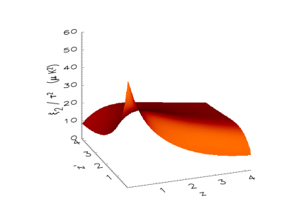
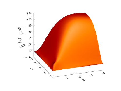
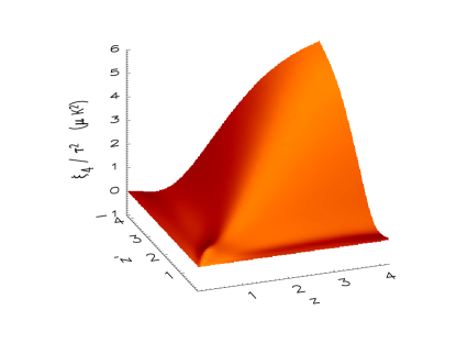
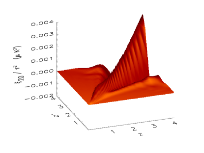
Figure 1: Correlation functions $\xi_{l}$ for $l=2,3,4,20$.

It is straightforward to check from equation (11) that all coefficients $p_{lm}(r)$ are real. In the terminology of CMB polarization Kamionkowski et al. (1997); Zaldarriaga and Seljak (1997), this means that the remote quadrupole data form an $E$-type spin-2 field at any given distance, with no $B$ modes. The absence of $B$ modes arises because we have considered only scalar perturbations as the source of the CMB quadrupole. If tensor perturbations were included, then in principle a $B$ component would arise. Considering the difficulty of detecting a remote quadrupole signal at all, the prospect of searching for a subdominant $B$-type signal sounds extremely daunting. It is probably more realistic, therefore, to search for the scalar ($E$-type) signal in such a survey, using the predicted absence of $B$ modes as a check on systematic errors and noise (see Section IV).

II.2 Correlations between clusters

Suppose that many clusters have been observed at many different positions ${\bf r}_{i}$. To determine the amount of information that can be obtained from such a survey, we need to know the correlations $\langle p({\bf r}_{i})p({\bf r}_{j})\rangle$. The full correlation function depends on the directions as well as the distances of the clusters Portsmouth (2004). The correlation functions are simpler to work with in spherical harmonic space, as the orthogonality of the spherical harmonics implies that there are no correlations between $p_{LM}$ and $p_{L^{\prime}M^{\prime}}$:

$$\langle p_{LM}(r)p_{L^{\prime}M^{\prime}}^{*}(r^{\prime})\rangle=\xi_{L}(r,r^{\prime})\delta_{LL^{\prime}}\delta_{MM^{\prime}}.$$ (13)

The correlation function is

$$\xi_{L}(r,r^{\prime})=\langle p_{LM}(r)p_{LM}^{*}(r^{\prime})\rangle=$$

$$\int_{0}^{\infty}dk\,k^{2}\Delta_{2}(k;r)\Delta_{2}(k;r^{\prime})F_{L}(kr)F_{L}(kr^{\prime})P_{\Phi}(k),$$ (14)

where the power spectrum $P_{\Phi}$ is given by

$$\langle\delta_{\Phi}({\bf k})\delta^{*}_{\Phi}({\bf k}^{\prime})\rangle=P_{\Phi}(k)\delta^{(3)}({\bf k}-{\bf k}^{\prime}).$$ (15)

On the scales of interest, $P_{\Phi}(k)\propto k^{n-4}$ where $n\approx 1$ is the spectral index.

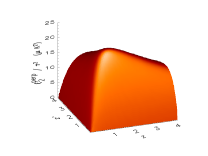
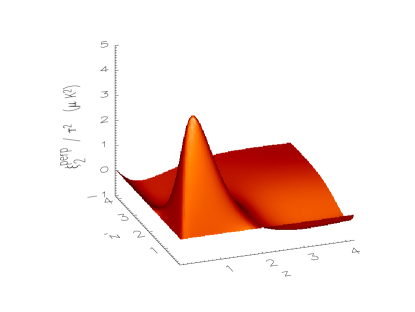
Figure 2: Correlation functions $\xi_{l}^{\perp}$ for $l=2$. In the left panel, only the correlation with the local temperature quadrupole has been projected out. In the right panel, the correlation with the polarization quadrupole has also been removed.

Fig. 1 shows the correlation functions $\xi_{l}$ for several values of $l$. In calculating the ISW integral and in converting from distance $r$ to redshift $z$, a flat Friedmann-Robertson-Walker cosmology with $\Omega_{m}=0.3$ and $\Omega_{\Lambda}=0.7$ was assumed. The results are normalized to WMAP on large angular scales. At low $l$, the correlations are extremely broad, meaning that even a survey covering a wide range of distances will contain few independent modes per $(l,m)$, as we will see in section III.2.

Remote quadrupole measurements are in general correlated with the local CMB anisotropy and polarization. To assess how much independent information is contained in the remote measurements, we need to know how strong these correlations are. Let us begin by considering correlations with the locally-measured temperature anisotropy. If the anisotropy spherical harmonic coefficients are $a_{lm}$, then the cross-correlation is

$$\zeta_{L}(r) \equiv\langle p_{LM}(r)a_{LM}^{*}\rangle$$ (16)

$$=\int_{0}^{\infty}dk\,k^{2}\Delta_{2}(k;r)\Delta_{L}(k;0)F_{L}(kr)P_{\Phi}(k),$$ (17)

where $\Delta_{L}$ is the appropriate transfer function.

If we wish to study only the information in a remote quadrupole data set that is independent of the local anisotropy, then we should project the mode coefficients onto the space orthogonal to that probed by the local CMB:

$$p_{LM}^{\perp}(r)=p_{LM}(r)-\frac{\zeta_{L}(r)}{C_{L}}a_{LM},$$ (18)

where $C_{l}\equiv\langle a_{lm}a_{lm}^{*}\rangle$ is the usual CMB angular power spectrum.

We can define a correlation function $\zeta_{L}^{E}$ and perform a similar projection to remove the portion of the signal that is correlated with the CMB polarization anisotropy coefficients $a_{lm}^{E}$. (There is no significant correlation with the $B$-type CMB polarization.) In performing this projection, it is important to include the effects of reionization, as most of the low-$l$ polarization signal comes from post-reionization scattering.

Fig. 2 shows the correlation functions $\xi^{\perp}_{l}$ corresponding to the projected coefficients $p_{lm}^{\perp}$ for $l=2$. As we will see, the difference between $\xi_{l}$ and $\xi_{l}^{\perp}$ decreases at higher $l$’s. In performing the projection, the Universe was assumed to have completely reionized at $z=11$, but the results do not depend strongly on the details of reionization, unless there was considerable patchiness on large scales.

The r.m.s. power due to all modes at a given $l$ is

$$p_{l}(r)=\sqrt{\frac{2l+1}{4\pi}\xi_{l}(r,r)},$$ (19)

and similarly for $p_{l}^{\perp}$. As Fig. 3 indicates, the quadrupole $l=2$ dominates the unprojected power at low redshift, but power shifts to smaller angular scales (higher $l$) as the redshift increases. At $l=2$, the projected power is much less than the unprojected power at all redshifts: the modes $p_{2m}$ are strongly correlated with the local temperature quadrupole at low $z$ and with the polarization quadrupole at high $z$. Modes with $l>2$ are comparatively weakly correlated with the local signals over some redshift ranges.

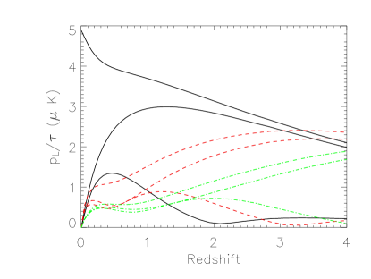
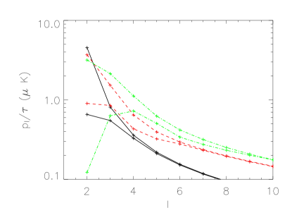
Figure 3: The r.m.s. signal per multipole. The left panel shows the signal in modes $l=2$ (solid, black), 3 (dashed, red), and 4 (dot-dashed, green) as a function of redshift. The bumps at $z\lesssim 0.5$ are due to the ISW effect. In each case, the three curves from top to bottom are the total signal, the result of projecting out the correlation with temperature quadrupole, and the result of projecting out both temperature and polarization. The right panel shows the signal as a function of $l$ for redshifts $z=0.1$ (solid, black) 1 (dashed, red), and 2 (dot-dashed, green). The upper curve is total signal, and the lower curve is the result of projecting out the correlations with local temperature and polarization.

.

All correlation functions except $\xi_{2}$ go to zero as $z,z^{\prime}\to 0$. This is expected: at low redshift, the remote quadrupole $p({\bf r})$ contains precisely the same information as the local quadrupole coefficients $a_{2m}$, so it must transform as a quadrupole itself. Indeed, it is straightforward to check from equation (11) that

$$p_{lm}(r)\to N\sqrt{\frac{4\pi}{5}}a_{lm}\delta_{l2}\qquad\mbox{as $r\to 0$}.$$ (20)

The real-space correlation functions are easily computed from the spherical harmonic space functions. The correlation between remote quadrupole signals of two clusters at locations ${\bf r}_{1},{\bf r}_{2}$ is

$$\langle p({\bf r}_{1})p({\bf r}_{2})\rangle=\sum_{L=2}^{\infty}\frac{2L+1}{4\pi}\xi_{L}(r_{1},r_{2})P_{L}(\hat{\bf r}_{1}\cdot\hat{\bf r}_{2})$$ (21)

using equations (8) and (13) and the spherical harmonic addition theorem. Similarly, the correlation between a remote quadrupole measurement $p({\bf r}_{1})$ and the local CMB $(\Delta T/T)({\bf r}_{2})$ is

$$\langle p({\bf r}_{1})(\Delta T/T)(\hat{\bf r}_{2})\rangle=\sum_{L=2}^{\infty}\frac{2L+1}{4\pi}\zeta_{L}(r_{1})P_{L}(\hat{\bf r}_{1}\cdot\hat{\bf r}_{2}).$$ (22)

Once the initial investment of calculating the $l$-space correlation functions has been made, these formulae allow rapid calculation of real-space correlations.

III Scales probed by remote quadrupole surveys

III.1 Survey at a fixed redshift

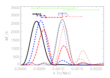
Figure 4: Window functions. The quantity $W_{l}^{2}/k$, which is proportional to the mean-square power in multipole a given multipole, is shown for a survey at $z=2$ for $l=2$ (solid, black), 3 (dashed, blue), and 4 (dot-dashed, red). In each case, the left (thicker) curve is the window function for the total signal $p_{lm}$, and the right (thinner) curve is the window function for $p_{lm}^{\perp}$. All functions are normalized to integrate to one. The bars above each window function show the 25th, 50th, and 75th percentiles. The green bars at the top of the plot indicate the percentiles for the $l=2$ and $l=10$ multipoles of the local CMB anisotropy.

We next examine the length scales probed by the various multipoles, assuming an all-sky survey has been used to estimate the coefficients $p_{lm}$ at some fixed redshift. We can write the signal as

$$p_{l}^{2}(r)=\int dk\,k^{2}P_{\Phi}(k)W_{l}^{2}(k;r),$$ (23)

with $W_{l}(k;r)=\frac{2l+1}{4\pi}\Delta_{2}(k;r)F_{l}(kr)$. Since $P_{\Phi}\propto k^{-3}$, the quantity $W_{l}^{2}/k$ is proportional to the power per wavenumber interval $dk$. Similarly, we can define a window function for the quantity $p_{l}^{\perp}$ that results from projecting out the part of the signal that is correlated with the local CMB.

The first few window functions are shown in Fig. 4 for $z=2$. Window functions corresponding to both $p_{l}$ and $p_{l}^{\perp}$ are shown. The range of scales probed by the various window functions are indicated with horizontal error bars, and for comparison the ranges corresponding to the local CMB power spectrum $C_{2}$ and $C_{10}$ are also indicated. Because of the ISW effect, the local CMB window functions are quite broad.

The first few unprojected modes probe scales as large as the CMB quadrupole but with narrower window functions. As noted earlier, these are significantly correlated with the local CMB polarization multipoles. Nonetheless, considering the likelihood that large-angle CMB polarization multipoles may be contaminated by foregrounds or systematic errors, the unprojected modes will still provide valuable new information on the largest-scale perturbations in the Universe, or at least test our understanding of large-angle polarization data. (The remote quadrupole survey will of course be susceptible to systematic errors and foregrounds as well, but the susceptibility will be different from that of the local polarization multipoles.)

The projected modes probe smaller scales, but they are still in the gigaparsec range, comparable to the first 10 or so CMB multipoles, and in some cases have narrow window functions. In practice, the projected modes at $l=2$ ($p_{2}^{\perp}$) are unlikely to be reliably measured, because the correlations are so strong, but projected modes with $l\geq 3$ will allow us to probe these large scales.

Fig. 5 shows the r.m.s. power $p_{l}$ and $p_{l}^{\perp}$ per multipole, plotted against the effective scale for each multipole. In interpreting this plot, bear in mind that each point represents the r.m.s. signal from all $2l+1$ modes at a given $l$.

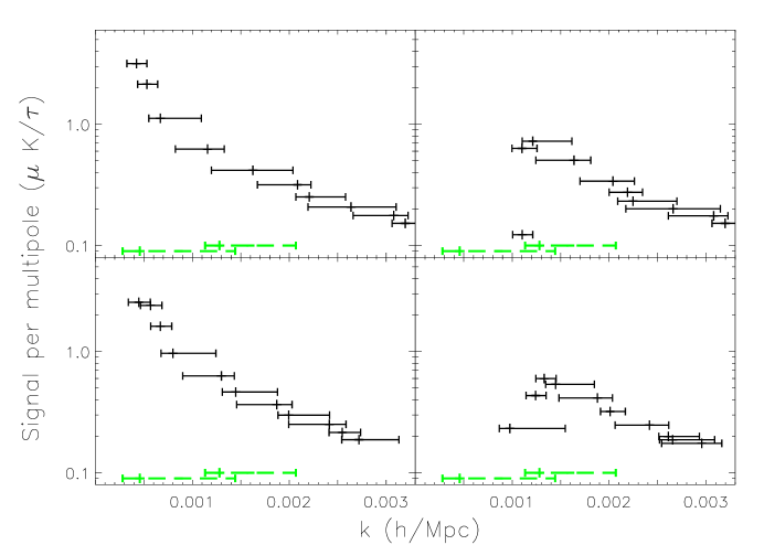
Figure 5: The r.m.s. signal vs. effective length scale. The upper plots are for a survey at $z=2$, and the lower plots are for $z=3$. On the left the total signal $p_{l}$ is shown, and on the right is the projected signal $p_{l}^{\perp}$. The horizontal error bars indicate 25th, 50th, 75th percentile contributions to the signal. Multipole $l$ increases from left to right within each plot. The dashed green bars at the bottom indicate the window functions for the local CMB anisotropy at $l=2$ and $l=10$; the vertical position of these bars is arbitrary.

In order to measure the quantities $p_{l}^{\perp}$, in principle we need an all-sky cluster survey, knowledge of the local CMB anisotropy and polarization spherical harmonic coefficients, and knowledge of the correlation functions $\zeta_{l}(r)$ and $\zeta_{l}^{E}(r)$ in order to project out the local contribution. In practice, of course, difficulties are likely with all of these. Section IV contains some discussion of how to mitigate these problems. For the moment, observe that information on large physical scales is found at large angular scales. We must survey a large fraction of the sky if we want to address the puzzles in the large-scale CMB with this technique. However, note that at redshifts $z=2$-3 the signal drops fairly rapidly as a function of $l$. This is good news: it means that a relatively sparse survey can measure the low-$l$ modes without excessive contamination from small angular scales.

III.2 Volume-limited survey

In the previous subsection, we considered surveys at a fixed redshift. We now imagine a volume-limited survey out to some maximum redshift $z_{\rm max}$. Let us continue to assume an all-sky survey, so that it is natural to think of the survey in spherical harmonic space. In this case, our survey provides estimates of each of the functions $p_{lm}(r)$ at multiple values of $r$.

For each $l$, we can enumerate a list of signal strength eigenmodes $\psi_{nl}$ that are solutions to

$$\int_{0}^{z_{\rm max}}\xi_{l}(r,r^{\prime})\psi_{nl}(r^{\prime})\,r^{\prime 2}\,dr^{\prime}=\lambda_{nl}\psi_{nl}(r).$$ (24)

The mode functions $\psi_{nl}(r)\ {}_{2}Y_{lm}(\hat{\bf r})$ form an orthonormal basis, which we can use to express the signal $p({\bf r})$. The mean-square signal in each mode is the eigenvalue $\lambda_{nl}$, so these modes provide a useful guide to tell us where the signal is strong.

For each mode, we can calculate a window function and hence assign a range of wavenumbers probed as we did for the surveys at fixed redshift. Results are illustrated in Fig. 6.

As one would expect, the mode with highest signal at each $l$ corresponds to a simple weighted average of $p_{lm}$ as a function of $r$ with positive weight everywhere. The next mode is essentially a difference between low- and high-redshift signals, and subsequent modes contain more radial oscillations. As Fig. 6 indicates, only the first couple of modes are likely to be measurable at any given $(l,m)$. Once again, the $l=2$ modes are strongly correlated with the local CMB polarization. Assuming the large-angle CMB polarization has been well measured, they provide relatively little new information; modes with $l\geq 3$ are the richest source of independent data on large-scale perturbations. On the other hand, if the first few CMB polarization multipoles are uncertain due to foregrounds or systematic errors, then the $l=2$ modes of a remote quadrupole survey may help to fill in this gap.

A comparison of Figs. 5 and 6 shows that significantly more large-scale information can be obtained from a volume-limited survey than from a survey on a shell. There is, of course, an obvious price to pay: many more clusters must be observed to estimate all these modes.

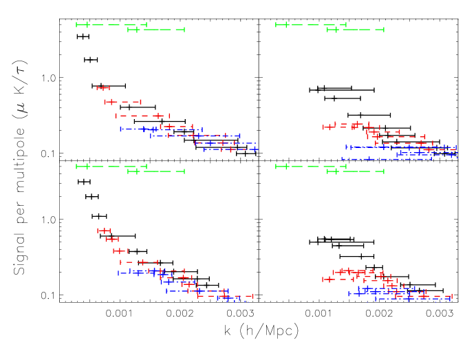
Figure 6: The r.m.s. signal vs. effective length scale. The upper panels show the results of a survey out to a maximum redshift of 2, and the lower panels are for a maximum redshift of 3. The total signal $p_{l}$ is plotted on the left, and the projected signal $p_{l}^{\perp}$ is on the right. The horizontal axis indicates the length scales of each mode as in Fig. 5. Solid black bars are the highest signal-strength eigenmode as a function of $l$. The dashed red bars are the second mode for each $l$, and the dot-dashed blue bars are the third mode. Multipole $l$ increases from left to right within each category. The long-dashed green bars at the top indicate the window functions for the local CMB anisotropy at $l=2$ and $l=10$; the vertical position of these bars is arbitrary.

IV Discussion

We have seen that an all-sky survey can probe the gigaparsec-scale Universe, measuring fluctuation modes that are independent of the local CMB. In surveys at redshifts around 2-3, the large-angular scale modes provide data on perturbations on the same length scales as the first few CMB multipoles, but with quite narrow window functions.

The results shown in the previous section were for an idealized survey: in addition to full sky coverage, the local CMB anisotropy coefficients $a_{lm}$ and the cross-correlations $\zeta_{l}(r)$, as well as the corresponding quantities for polarization, were assumed to be known in order to compute the projected signal $p_{lm}^{\perp}$. We must ask what happens if these assumptions are replaced by more realistic ones. The most complete way to answer these questions would be to assume a precise survey geometry and compute the resulting Fisher matrix. We will not perform such a detailed analysis here; we can, however, make some general observations.

In a survey that covers a fraction of the sky $f_{\rm sky}$, only band powers with width $\Delta l\sim f_{\rm sky}^{-1/2}$ can be recovered, not individual multipoles. Furthermore, the lowest-$l$ modes cannot be recovered at all. For the goal of probing the largest scales, therefore, large sky coverage is essential independent of the choice of redshift. A survey with $f_{\rm sky}=0.1$, for instance (4000 square degrees) would be able to recover only a single mode in the $l=2$-$3$ band.

On the other hand, the power drops fairly rapidly as a function of $l$, so contamination of the low-$l$ modes from high-$l$ power is modest. In other words, in order to probe large scales, we should survey as much sky as possible, but the survey can be sparse.

Next, let us consider uncertainties in projecting out the local CMB contribution (i.e., going from $p_{lm}$ to $p_{lm}^{\perp}$). For all $l>2$, this projection is subdominant to the primary signal over some range of redshifts, so independent information should be obtainable from these modes.

The $l=2$ modes are a different matter, as the correlations are extremely strong there. As Fig. 3 indicates, the projected coefficients $p_{2m}^{\perp}$ are much smaller than the unprojected coefficients $p_{2m}$ at all redshifts. At low redshift, the culprit is the temperature quadrupole, while at high redshift $p_{2m}$ becomes very strongly correlated with the polarization quadrupole. To put the situation pessimistically, accurate extraction of $p_{2m}^{\perp}(r)$ may never be feasible. To extract information about large-scale perturbations that is independent of the local CMB, we will look to modes $p_{lm}$ with $l\geq 3$ (or, in the case of a partial-sky survey, by modes that cover the largest available angular scales but are orthogonal to the quadrupole).

A more optimistic interpretation is that measurement of $p_{2m}$ at a couple of different redshifts can allow us to determine the local CMB temperature and polarization quadrupole coefficients (that is, the 5 coefficients $a_{2m}$ and the 5 coefficients $a_{2m}^{E}$). Since direct measurements of these coefficients may be contaminated by foregrounds or systematic errors (especially in the case of polarization), such an independent determination of these coefficients will be important in assessing the significance of the large-scale anomalies in the CMB. Furthermore, by measuring $p_{2m}$ as a function of redshift, we may be able to test our theoretical predictions of the cross-correlation functions $\zeta_{2},\zeta_{2}^{E}$, thus providing a probe of the recent ISW effect.

A common question is whether a remote quadrupole survey can “beat cosmic variance.” The answer depends on precisely what we mean by this phrase. Fig. 7 provides one possible answer. The figure shows the cumulative number of independent modes on scales larger than a given value for ideal all-sky surveys out to a specified redshift. All of the signal eigenmodes are included in this count. The number of modes contained in the all-sky CMB temperature anisotropy data (without polarization) is shown for comparison. Although a survey that went all the way out to $z=\infty$ would “beat” the local CMB, realistic surveys never do. The amount of new information can be comparable, however, on some scales. In particular, the number of new modes obtainable by a remote quadrupole survey in the range $k\sim 0.002h/$Mpc is about the same as that contained in the local CMB (because the slopes of the cumulative curves in Fig. 7 are about the same there). Considering the unsettled state of our understanding of gigaparsec-scale perturbations and the hints that something surprising may be going on there, it is clear that there is valuable information to be gained.

This article has focused primarily on the largest-scale information contained in remote cluster surveys. The formalism described here is also useful for surveys designed to probe the ISW effect Baumann and Cooray (2003); Cooray and Baumann (2003); Cooray et al. (2004); Seto and Pierpaoli (2005). Such surveys provide a powerful probe of the recent growth of structure and hence may shed light on the nature of dark energy and the growth of structure. Because the ISW effect is most important at low redshift (see Fig. 3), such a survey will be quite different from those considered here: the best approach appears to be a denser survey of a smaller area of the sky at low redshift. In planning a survey to probe the ISW effect, it will be important to quantify the number of independent modes that can be probed. The detailed answer will depend on the precise locations of the clusters to be surveyed, but a simple estimate obtained by counting modes in spherical harmonic space and scaling by $f_{\rm sky}^{-1/2}$ should provide valuable guidance.

Clusters are of course not randomly distributed “test particles”: they are overdensities. One might worry that this would lead to biases in the modes recovered from such a survey. A remote quadrupole survey (even a small-scale one optimized for characterizing the ISW) primarily probes scales of several hundred Mpc or more, which is considerably larger than the scale associated with the formation of individual clusters. One would therefore not expect significant bias due to the locations of individual clusters. On the other hand, the modes recovered from such a survey would presumably be correlated with tracers of large-scale structure on hundred-Mpc scales. In analyzing the results of such a future survey, one would want to characterize those correlations, presumably via $N$-body simulations. For the gigaparsec-scale surveys that are the primary focus of this paper, of course, clusters can be taken as randomly-distributed test particles.

In a detailed Fisher-matrix analysis of a potential survey, the real-space covariance matrix $\langle p({\bf r}_{i})p({\bf r}_{j})\rangle$ will be needed, as will the correlation with the local CMB. The formalism in this paper provides a useful way to compute these quantities. The full covariance matrix can be computed with and without the ISW effect, and Fisher matrix estimates of the errors with which ISW parameters can be reconstructed can be computed quickly and easily for any desired survey geometry.

A survey of the sort considered here will surely be a daunting task. The signals are sub-microkelvin, and there is unfortunately no shortage of confusing signals. Some signals (diffuse Galactic foregrounds and the kinematic signal due to the cluster’s peculiar velocity) can be distinguished by their spectral signature, assuming a multifrequency survey, but detailed information on the spectral and spatial properties of polarized foregrounds will be necessary. The three-year WMAP data have advanced the state of knowledge in this area considerably Page et al. (2006), and further information will come from the Planck satellite Tauber (2004) as well as ground-based experiments.

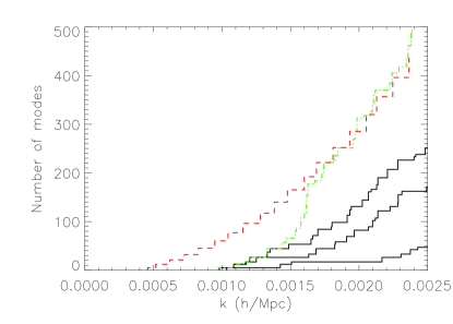
Figure 7: The cumulative number of modes as a function of scale. From bottom to top, the solid curves show predictions for surveys with $z_{\rm max}=1,2,3$. The red dashed curve shows the number of modes probed by the local CMB anisotropy, and the green dotted curve shows the results of a hypothetical remote quadrupole all-sky survey out to $z=\infty$.

Of potentially greater concern is the intrinsic CMB polarization (both due to last scattering and reionization), which will be lensed by the cluster itself. In order for the remote quadrupole survey to be detectable, we will probably need detailed knowledge of the cluster optical depth as a function of position on the sky, and possibly the projected mass density as well. With this information, we can construct a template for the remote quadrupole signal and use it to fit for the two parameters that determine the remote quadrupole at that cluster [$Q$ and $U$ or equivalently the real and imaginary parts of $p({\bf r})$]. Since the background polarization is not expected to be spatially correlated with this template, this will help in separating the signal from the confusing background. In the near future, Sunyaev-Zel’dovich surveys will provide a wealth of detailed cluster data Ruhl et al. (2004); Kosowsky (2003), so there is reason to hope that such an approach may soon be feasible.

In any remote quadrupole survey, assessment of the errors will be crucial. For instance, errors in determining the optical depths $\tau$ of the clusters can induce spurious signals. Just as in the case of CMB polarization maps, a valuable diagnostic can be obtained by considering the decomposition of the data into $E$ and $B$ modes Kamionkowski et al. (1997); Zaldarriaga and Seljak (1997). At any fixed redshift $z$, the remote quadrupole data consist of a spin-2 field on the sphere that is derived from a scalar perturbation (assuming that primordial tensor perturbations can be neglected). As noted in Section II, the true signal — everything calculated in this paper — should therefore consist only of $E$ modes, precisely as in the case of scalar perturbations in the CMB. Noise and systematic errors, on the other hand, are likely to populate E and B equally Zaldarriaga (2001). When analyzing results of an actual survey, therefore, the B modes can be monitored to determine the errors. In practice, for a partial-sky survey with sparse sampling, there will be significant $E$-$B$ mixing Lewis et al. (2002); Bunn (2002a, b); Bunn et al. (2003), but this technique should still provide a valuable check.

Acknowledgments:

This work was supported by NSF Grants 0233969 and 0507395 and by a Cottrell Award from the Research Corporation. I thank Max Tegmark and the MIT physics department for their hospitality during the completion of this work, and an anonymous referee for helpful comments.

Appendix A

In this section we derive some identities involving spherical harmonics, coordinate transforms, and 3-$j$ symbols.

A.1 Rotation matrices and spin-2 spherical harmonics.

For a given cluster location ${\bf r}$, we adopt a primed coordinate system obtained by rotating the $z$ axis until it points in the direction $\hat{\bf r}$. Let $R$ be the rotation that relates the two coordinate systems. The Euler angles associated with this rotation are $(\phi_{\hat{\bf r}},\theta_{\hat{\bf r}},0)$, using the same conventions as Lewis et al. (2002). The spherical harmonic $Y_{22}$ in the primed coordinate system can be expressed in the unprimed coordinates as

$$Y_{22}(\hat{\bf k}^{\prime})=\sum_{m=-2}^{2}D^{2}_{m2}(R)Y_{2m}(\hat{\bf k}),$$ (25)

where $D^{l}_{mm^{\prime}}(R)$ is the Wigner matrix for the rotation $R$. The Wigner matrices can be expressed in terms of spin-$s$ spherical harmonics Lewis et al. (2002):

$$D^{l}_{-ms}(\phi,\theta,-\psi)=(-1)^{m}\sqrt{\frac{4\pi}{2l+1}}\ {}_{s}Y_{lm}(\theta,\phi)e^{is\psi}.$$ (26)

The result is

$$Y_{22}(\hat{\bf k}^{\prime})=\sqrt{\frac{4\pi}{5}}\sum_{m}(-1)^{m}{}_{2}Y_{2-m}(\hat{\bf r})Y_{2m}(\hat{\bf k}).$$ (27)

A.2 Integrals over spherical harmonics.

The derivation in Section II contains an integral

$$I\equiv\int d^{2}\hat{\bf r}\ {}_{2}Y_{2-m}(\hat{\bf r})\ {}_{2}Y_{LM}^{*}(\hat{\bf r})e^{i{\bf k}\cdot{\bf r}}.$$ (28)

To evaluate this integral, we expand the exponential in spherical harmonics to get

$$I=4\pi\sum_{\lambda,\mu}i^{\lambda}j_{\lambda}(kr)Y_{\lambda\mu}(\hat{\bf k})\int d^{2}\hat{\bf r}\,Y_{\lambda\mu}^{*}(\hat{\bf r})\ {}_{2}Y_{2-m}(\hat{\bf r})\ {}_{2}Y_{LM}^{*}(\hat{\bf r}).$$ (29)

Next, we want to evaluate the integral over the three spherical harmonics. Using the identity ${}_{s}Y_{lm}^{*}=(-1)^{m+s}\,{}_{-s}Y_{l-m}$, the integral we need can be written in the form

$$J\equiv\int d^{2}\hat{\bf r}\ {}_{2}Y_{l_{1}m_{1}}(\hat{\bf r})\ {}_{-2}Y_{l_{2}m_{2}}(\hat{\bf r})Y_{l_{3}m_{3}}(\hat{\bf r}).$$ (30)

Equation (B3) of Lewis et al. (2002) tells us how to express all of the spherical harmonics in terms of $D$-matrices:

$$J=\sqrt{\frac{(2l_{1}+1)(2l_{2}+1)(2l_{3}+1)}{(4\pi)^{3}}}\int d^{2}\hat{\bf r}\ D^{l_{1}}_{-m_{1}2}D^{l_{2}}_{-m_{2}2}D^{l_{3}}_{-m_{3}0}.$$ (31)

Here the $D$-matrices can be evaluated for any rotation $R(\phi,\theta,\psi)$ with the first two Euler angles being the spherical coordinates of $\hat{\bf r}$. Since the integrand doesn’t depend on the third Euler angle $\psi$, we can replace $\int d^{2}\hat{\bf r}$ with $\frac{1}{2\pi}\int d^{3}R$, an integral over the entire rotation group. Zare Zare (1988) (p. 103) gives this integral in terms of $3j$ symbols:

$$J=\sqrt{\frac{(2l_{1}+1)(2l_{2}+1)(2l_{3}+1)}{4\pi}}\begin{pmatrix}l_{1}&l_{2}&l_{3}\\ -m_{1}&-m_{2}&-m_{3}\end{pmatrix}\begin{pmatrix}l_{1}&l_{2}&l_{3}\\ 2&-2&0\end{pmatrix}.$$ (32)

So we can write the integral in equation (28) as

$$I=\sum_{\lambda,\mu}i^{\lambda}(-1)^{m}j_{\lambda}(kr)Y_{\lambda\mu}(\hat{\bf k})\sqrt{20\pi(2\lambda+1)(2L+1)}\begin{pmatrix}2&L&\lambda\\ 2&-2&0\end{pmatrix}\begin{pmatrix}2&L&\lambda\\ m&M&\mu\end{pmatrix}.$$ (33)

We can use this result to write equation (10) as

$$p_{LM}(r)=4\pi N\int d^{3}k\,\Delta_{2}(k;r)\delta_{\Phi}({\bf k})\sum_{\lambda}i^{\lambda}\sqrt{(2L+1)(2\lambda+1)}j_{\lambda}(kr)\begin{pmatrix}2&L&\lambda\\ 2&-2&0\end{pmatrix}K(\hat{\bf k}),$$ (34)

where

$$K(\hat{\bf k})=\sum_{m,\mu}\begin{pmatrix}2&L&\lambda\\ m&M&\mu\end{pmatrix}Y_{\lambda\mu}(\hat{\bf k})Y_{2m}(\hat{\bf k}).$$ (35)

Expand $K$ in spherical harmonics: $K(\hat{\bf k})=\sum_{l_{0}m_{0}}K_{l_{0}m_{0}}Y_{l_{0}m_{0}}(\hat{\bf k})$. The coefficients are

$$K_{l_{0}m_{0}} =\sum_{m,\mu}\begin{pmatrix}2&L&\lambda\\ m&M&\mu\end{pmatrix}\int d^{2}\hat{\bf k}\,Y_{2m}(\hat{\bf k})Y_{\lambda\mu}(\hat{\bf k})Y_{l_{0}m_{0}}^{*}(\hat{\bf k})$$ (36)

$$=(-1)^{m_{0}}\sum_{m,\mu}\begin{pmatrix}2&L&\lambda\\ m&M&\mu\end{pmatrix}\sqrt{\frac{5(2l_{0}+1)(2\lambda+1)}{4\pi}}\begin{pmatrix}2&l_{0}&\lambda\\ 0&0&0\end{pmatrix}\begin{pmatrix}2&l_{0}&\lambda\\ m&-m_{0}&\mu\end{pmatrix}$$ (37)

$$=\frac{(-1)^{m_{0}}}{2L+1}\sqrt{\frac{5(2l_{0}+1)(2\lambda+1)}{4\pi}}\begin{pmatrix}2&l_{0}&\lambda\\ 0&0&0\end{pmatrix}\delta_{Ll_{0}}\delta_{M,-m_{0}},$$ (38)

using equation (3.119) in Zare (1988) to integrate the product of three spherical harmonics, and then using the orthogonality of the 3-$j$ symbols [equation (2.32) in Zare (1988)]. So $K$ has only one term in its spherical harmonic expansion: $K(\hat{\bf k})=K_{L-M}Y_{L-M}(\hat{\bf k})$. Substituting this into equation (34), we get

$$p_{LM}(r)=N\sqrt{20\pi}\sum_{\lambda}i^{\lambda}(2\lambda+1)\begin{pmatrix}2&L&\lambda\\ 2&-2&0\end{pmatrix}\begin{pmatrix}2&L&\lambda\\ 0&0&0\end{pmatrix}\int d^{3}k\,\Delta_{2}(k;r)\delta_{\Phi}({\bf k})j_{\lambda}(kr)Y_{LM}^{*}(\hat{\bf k}).$$ (39)

The 3-$j$ symbols vanish whenever the triangle inequality is not satisfied, so $\lambda$ must be between $L-2$ and $L+2$. Furthermore, $\left(\begin{smallmatrix}2&L&\lambda\\ 0&0&0\end{smallmatrix}\right)=0$ when $2+L+\lambda$ is odd. So the sum above contains only three terms: $\lambda=L-2,L,L+2$.

References

- Bennett et al. (2003) C. L. Bennett, M. Halpern, G. Hinshaw, N. Jarosik, A. Kogut, M. Limon, S. S. Meyer, L. Page, D. N. Spergel, G. S. Tucker, et al., Astrophys. J. Supp. 148, 1 (2003).
- Hinshaw et al. (2003) G. Hinshaw, D. N. Spergel, L. Verde, R. S. Hill, S. S. Meyer, C. Barnes, C. L. Bennett, M. Halpern, N. Jarosik, A. Kogut, et al., Astrophys. J. Supp. 148, 135 (2003).
- Kogut et al. (2003) A. Kogut, D. N. Spergel, C. Barnes, C. L. Bennett, M. Halpern, G. Hinshaw, N. Jarosik, M. Limon, S. S. Meyer, L. Page, et al., Astrophys. J. Supp. 148, 161 (2003).
- Hinshaw et al. (2006) G. Hinshaw, M. Nolta, C. Bennett, R. Bean, O. Doré, M. Greason, M. Halpern, R. Hill, N. Jarosik, A. Kogut, et al., ArXiv Astrophysics e-prints (2006), eprint arXiv:astro-ph/0603451.
- Page et al. (2006) L. Page, G. Hinshaw, E. Komatsu, M. Nolta, D. Spergel, C. Bennett, C. Barnes, R. Bean, O. Doré, M. Halpern, et al., ArXiv Astrophysics e-prints (2006), eprint arXiv:astro-ph/0603450.
- Spergel et al. (2006) D. Spergel, R. Bean, O. Doré, M. Nolta, C. Bennett, G. Hinshaw, N. Jarosik, E. Komatsu, L. Page, H. Peiris, et al., ArXiv Astrophysics e-prints (2006), eprint arXiv:astro-ph/0603449.
- Bennett et al. (1996) C. L. Bennett, A. J. Banday, K. M. Gorski, G. Hinshaw, P. Jackson, P. Keegstra, A. Kogut, G. F. Smoot, D. T. Wilkinson, and E. L. Wright, Astrophys. J. Lett. 464, L1 (1996).
- Gorski et al. (1996) K. M. Gorski, A. J. Banday, C. L. Bennett, G. Hinshaw, A. Kogut, G. F. Smoot, and E. L. Wright, Astrophys. J. Lett. 464, L11 (1996).
- Hinshaw et al. (1996) G. Hinshaw, A. J. Branday, C. L. Bennett, K. M. Gorski, A. Kogut, C. H. Lineweaver, G. F. Smoot, and E. L. Wright, Astrophys. J. Lett. 464, L25 (1996).
- de Oliveira-Costa et al. (2004) A. de Oliveira-Costa, M. Tegmark, M. Zaldarriaga, and A. Hamilton, Phys. Rev. D 69, 063516 (2004).
- Copi et al. (2004) C. J. Copi, D. Huterer, and G. D. Starkman, Phys. Rev. D 70, 043515 (2004).
- Schwarz et al. (2004) D. J. Schwarz, G. D. Starkman, D. Huterer, and C. J. Copi, Phys. Rev. Lett. 93, 221301 (2004).
- Hansen et al. (2004) F. K. Hansen, A. J. Banday, and K. M. Górski, M.N.R.A.S. 354, 641 (2004).
- Land and Magueijo (2005) K. Land and J. Magueijo, Phys. Rev. Lett. 95, 071301 (2005).
- Bernui et al. (2005) A. Bernui, B. Mota, M. J. Reboucas, and R. Tavakol, ArXiv Astrophysics e-prints (2005), eprint arXiv:astro-ph/0511666.
- Bielewicz et al. (2005) P. Bielewicz, H. K. Eriksen, A. J. Banday, K. M. Górski, and P. B. Lilje, Astrophys. J. 635, 750 (2005).
- Copi et al. (2006) C. J. Copi, D. Huterer, D. J. Schwarz, and G. D. Starkman, M.N.R.A.S. 367, 79 (2006), eprint astro-ph/0508047.
- Bernui et al. (2006) A. Bernui, T. Villela, C. A. Wuensche, R. Leonardi, and I. Ferreira, ArXiv Astrophysics e-prints (2006), eprint arXiv:astro-ph/0601593.
- Efstathiou (2003) G. Efstathiou, M.N.R.A.S. 346, L26 (2003).
- Doré et al. (2004) O. Doré, G. P. Holder, and A. Loeb, Astrophys. J. 612, 81 (2004).
- Skordis and Silk (2004) C. Skordis and J. Silk, ArXiv Astrophysics e-prints (2004), eprint arXiv:astro-ph/0402474.
- Sazonov and Sunyaev (1999) S. Y. Sazonov and R. A. Sunyaev, M.N.R.A.S. 310, 765 (1999).
- Kamionkowski and Loeb (1997) M. Kamionkowski and A. Loeb, Phys. Rev. D 56, 4511 (1997).
- Seto and Pierpaoli (2005) N. Seto and E. Pierpaoli, Phys. Rev. Lett. 95, 101302 (2005).
- Baumann and Cooray (2003) D. Baumann and A. Cooray, New Astronomy Review 47, 839 (2003).
- Portsmouth (2004) J. Portsmouth, Phys. Rev. D 70, 063504 (2004).
- Cooray and Baumann (2003) A. Cooray and D. Baumann, Phys. Rev. D 67, 063505 (2003).
- Cooray et al. (2004) A. Cooray, D. Huterer, and D. Baumann, Phys. Rev. D 69, 027301 (2004).
- Sachs and Wolfe (1967) R. K. Sachs and A. M. Wolfe, Astrophys. J. 147, 73 (1967).
- Hu and Dodelson (2002) W. Hu and S. Dodelson, Ann. Rev. Astron. Astrophys. 40, 171 (2002).
- Challinor et al. (2000) A. D. Challinor, M. T. Ford, and A. N. Lasenby, M.N.R.A.S. 312, 159 (2000).
- Shimon et al. (2006) M. Shimon, Y. Rephaeli, B. W. O’Shea, and M. L. Norman, ArXiv Astrophysics e-prints (2006), eprint arXiv:astro-ph/0602528.
- Liu et al. (2005) G.-C. Liu, A. da Silva, and N. Aghanim, Astrophys. J. 621, 15 (2005).
- Padmanabhan (2003) T. Padmanabhan, Phys. Rep. 380, 235 (2003).
- Kamionkowski et al. (1997) M. Kamionkowski, A. Kosowsky, and A. Stebbins, Phys. Rev. D 55, 7368 (1997).
- Zaldarriaga and Seljak (1997) M. Zaldarriaga and U. Seljak, Phys. Rev. D 55, 1830 (1997).
- Tauber (2004) J. A. Tauber, Advances in Space Research 34, 491 (2004).
- Ruhl et al. (2004) J. Ruhl, P. Ade, J. Carlstrom, H. Cho, T. Crawford, M. Dobbs, C. Greer, N. Halverson, W. Holzapfel, T. Lantin, et al., Proc. SPIE 5498, 11 (2004).
- Kosowsky (2003) A. Kosowsky, New Astronomy Review 47, 939 (2003).
- Zaldarriaga (2001) M. Zaldarriaga, Phys. Rev. D 64, 103001 (2001).
- Lewis et al. (2002) A. Lewis, A. Challinor, and N. Turok, Phys. Rev. D 65, 023505 (2002).
- Bunn (2002a) E. F. Bunn, Phys. Rev. D 65, 043003 (2002a).
- Bunn (2002b) E. F. Bunn, Phys. Rev. D 66, 069902 (2002b).
- Bunn et al. (2003) E. F. Bunn, M. Zaldarriaga, M. Tegmark, and A. de Oliveira-Costa, Phys. Rev. D 67, 023501 (2003).
- Zare (1988) R. N. Zare, Angular momentum: Understanding spatial aspects in chemistry and physics (John Wiley & Sons, 1988).