Metal Enrichment of the ICM: a 3-D Picture of Chemical and Dynamical Properties

Abstract

We develop a model for the metal enrichment of the intracluster medium (ICM) that combines a cosmological non-radiative hydrodynamical N-Body/SPH simulation of a cluster of galaxies, and a semi-analytic model of galaxy formation. The novel feature of our hybrid model is that the chemical properties of the diffuse gas in the underlying simulation are dynamically and consistently generated from stars in the galaxies. We follow the production of several chemical elements, provided by low- and intermediate-mass stars, core collapse and type Ia supernovae. We analyse the spatial distribution of metals in the ICM, investigate the way in which the chemical enrichment proceeds, and use iron emissivity as a tracer of gas motions. The similar abundance patterns developed by O and Fe indicate that both types of SNe pollute the ICM in a similar fashion. Their radial abundance profiles are enhanced in the inner $100\,h^{-1}$ kpc in the last Gyr because of the convergence of enriched gas clumps to the cluster centre; this increment cannot be explained by the metal ejection of cluster galaxies which is quite low at the present epoch. Our results support a scenario in which part of the central intracluster gas comes from gas clumps that, in the redshift range of $z\sim 0.2$ to $\sim 0.5$, have been enriched to solar values and are at large distances from the cluster centre (from $\sim 1$ to $\sim 6\,h^{-1}$ Mpc) moving at very high velocities (from $\sim 1300$ to $\sim 2500\,{\rm km}\,{\rm s}^{-1}$). The turbulent gas motions within the cluster, originated in the inhomogeneous gas infall during the cluster assembly, are manifested in emission-weighted velocity maps as gradients that can be as large as $\sim 1000\,{\rm km}\,{\rm s}^{-1}$ over distances of a few hundred kpc. Gradients of this magnitude are also seen in velocity distributions along sightlines through the cluster centre. Doppler shifting and broadening suffered by the Fe ${\rm K}_{\alpha}$ 6.7 keV emission line along such sightlines could be used to probe these gas large-scale motions when they are produced within an area characterised by high iron line emissivity.

1 Introduction

Clusters of galaxies are the largest virialised objects in the Universe. Within the hierarchical structure formation scenario of the cold dark matter (CDM) model, they arise from the rare highest peaks of the initial density perturbation field. During cluster assembly, the dissipative gas component is shock heated by the potential well of the cluster, reaching very high temperatures ($T\sim 10^{7-8}$ K). This hot and diffuse gas radiates energy through thermal bremsstrahlung in the X-ray band of the electromagnetic spectrum. The gravitationally dominating collisionless dark matter component on the other hand shows considerable substructure, as revealed by high resolution simulations that follow cluster assembly (e.g. Springel et al. 2001 and references therein). These substructures are the surviving remnants of dark matter haloes that have fallen in at earlier times, and plausibly mark the location of the cluster galaxies.

X-ray observations have first revealed the presence of hot gas trapped in the potential well of galaxy clusters, and provide a wealth of information about the dynamical, thermal and chemical properties of clusters. A strong feature in their spectra is the presence of line emission produced by highly ionised iron, mainly, the H- and He-like iron lines at 6.9 and 6.7 keV. The content of iron in the intracluster medium (ICM) is approximately one third of the solar value (Fukazawa et al. 1998; Ettori, Allen & Fabian 2001), suggesting that some of its hot gas must have originated in the galaxies that reside in the cluster. The processes considered for the supply of this enriched gas include galactic winds driven by supernovae explosions (White 1991; Renzini 1997), ram pressure stripping (Mori & Burkert, 2000), early enrichment by hypernovae associated with population type III stars (Loewenstein, 2001), and intracluster stars (Zaritsky, Gonzalez & Zabludoff, 2004).

Spatially resolved maps of the temperature and metal abundance distributions in the intracluster medium have been obtained by X-ray surveys carried out with ROSAT, ASCA, BeppoSAX (Finoguenov, David & Ponman 2000; Finoguenov, Arnaud & David 2001; De Grandi & Molendi 2001), and more recently with XMM-Newton and Chandra (Gastaldello & Molendi 2002; Finoguenov et al. 2002; Sanders & Fabian 2002; Matsushita, Finoguenov & Böhringer 2003; Tamura et al. 2004). As a result, abundance profiles of several chemical species with different origins have been obtained, namely for O and Si generated by core collapse supernovae (SNe CC) and Fe, mainly produced by type Ia supernovae (SNe Ia). These profiles reflect physical mixing processes in the baryonic component due to gas cooling, star formation, metal production, and energetic and chemical feedback, all coupled to the hierarchical build up of the galaxies and the clusters. These observations can therefore be very valuable for constraining models of galaxy formation and chemical enrichment of the ICM, allowing to evaluate the relative importance of different types of supernovae for metal pollution. The spatial distribution of metals obtained from models of the ICM chemical enrichment can be analysed by constructing X-ray weighted metal maps which trace the interactions between the ICM and cluster galaxies; thus, when they are compared with observed metal maps, they provide information about the mechanisms involved in the enrichment process and may reveal the dynamical state of a galaxy cluster (Kapferer et al. 2005; Domainko et al. 2005).

X-ray observations also provide important information about the dynamics of the intracluster gas through radial velocity measurements in clusters (Dupke & Bregman, 2001), allowing in principle further tests of structure formation models. Gaseous bulk flows affect the characteristics of X-ray spectra of the ICM by Doppler broadening and shifting of emission lines. The prominent Fe ${\rm K}_{\alpha}$ 6.7 keV iron emission line present in X-ray spectra of galaxy clusters could be used as a tracer of these motions. This possibility was evaluated by Sunyaev et al. (2003), who showed that future X-ray missions like CONSTELLATION-X and XEUS, with an energy resolution of a few eV, should be able to detect several Doppler-shifted components of this emission line in the core of the cluster.

All this wealth of data calls for a theoretical interpretation of the ICM chemical enrichment in the framework of a detailed cluster formation model. The approaches used so far to this end include semi-analytic models of galaxy formation coupled to N-Body simulations of galaxy clusters (De Lucia, Kauffmann & White 2004; Nagashima et al. 2005), hydrodynamical simulations of cluster formation which include, self-consistently, star formation, SNe feedback and metal enrichment from SNe CC and Ia (e.g. Valdarnini 2003; Tornatore et al. 2004), and an intermediate approach that combines N-Body and hydrodynamic simulations together with a phenomenological galaxy formation model and a prescription of the effect under study, such as galactic winds and merger-driven starbursts (Kapferer et al., 2005) and ram-pressure stripping (Schindler et al., 2005; Domainko et al., 2005). In this work, we present a different intermediate approach which combines a cosmological non-radiative hydrodynamical N-Body/SPH simulation of a cluster of galaxies, with a semi-analytic model of galaxy formation. The simplicity of the semi-analytic model has the advantage of reaching a larger dynamic range than fully self-consistent hydro-simulations, at a far smaller computational cost. In particular, it allows us to explore more easily the range of parameters that characterise appropriate chemical enrichment models.

The long cooling time of the bulk of the gas in rich clusters justifies the assumption of a non-radiative gas (Evrard 1990; Frenk et al. 1999). However, this time-scale becomes smaller than the Hubble time in the core of the cluster, where the densities are higher. Here is where the semi-analytic model plays an important part, taking into account radiative cooling, and models for star formation, chemical enrichment and energetic feedback from galaxies. The semi-analytic model used here is based on previous works (Springel et al. 2001; De Lucia et al. 2004, DL04 hereafter), but was extended with a new chemical implementation that tracks the abundance of different species resulting from mass loss through stellar winds of low-, intermediate- and high-mass stars, and from the explosions of SNe CC and Ia supernovae. The principal new feature of our model is however the link between semi-analytic model results and the chemical enrichment of gas particles in the underlying N-Body/SPH simulation. We pollute gas particles with metals ejected from the galaxies, consistent with the modelling of the semi-analytic model. These metals are then carried around and mixed by the hydrodynamic processes during cluster formation. Thus, we are not limited to an analysis of mean chemical properties of the intracluster gas, like in the original model of DL04. Instead, the enrichment of gas particles allows a study of the spatial distribution of metals in the ICM, and to use iron emissivity as a tracer of gas motions.

The aim of our model is, on one hand, to understand the way in which the chemical enrichment patterns characterising the intracluster gas develop, and, on the other, to detect the imprints of gas bulk motions in the shape of X-ray emission lines, thus providing guidance for the interpretation of future spectroscopic X-ray data. The first part of the present study is therefore devoted to an analysis of chemical enrichment of the ICM, focusing on the spatial distribution of different chemical elements. In a second part we analyse the link between the occurrence of multiple components in the Fe ${\rm K}_{\alpha}$ 6.7 keV emission line and the range of velocities of the gas that generates this emission. This is directly relevant to the question whether metal emission-line-weighted velocity maps of the cluster could be used to infer the spatial coherence of these bulk motions. Gathering all the information available in the form of projected maps and detailed spectra along lines of sight through the ICM, we are able to extend the information in 2-D provided by observed projected distributions of gas temperature, abundances and surface brightness, into a 3-D picture of the ICM properties.

This paper is organised as follows. Section 2 describes our hybrid model used to study the ICM chemical enrichment, summarises the properties of the hydrodynamical simulation used and presents the main features of the semi-analytic model. Section 3 contains the details of the chemical model implemented in the semi-analytic model. It also describes the way in which metals released by stellar mass losses and supernovae explosions are spread among gas particles of the N-Body/SPH simulation. In Section 4, we fix the parameters that characterise our version of the semi-analytic model and compare its results with local observations. The following three sections present the main results of this work. Section 5 gives the radial abundance profiles of different chemical elements, comparing them with observations. In Section 6, we visualise the thermodynamical and chemical properties of the ICM by projecting the corresponding mass-weighted or emission-weighted related quantities. These two techniques (radial profiles and projected maps) are used to analyse the history of the ICM chemical enrichment as well as the dynamical evolution of the intracluster gas, as discussed in Section 7. Section 8 describes the use of Fe ${\rm K}_{\alpha}$ 6.7 keV emission line as a probe of the ICM dynamics. Finally, in Section 9, we give a summary and discussion of our results.

Throughout this paper we express our model chemical abundances in terms of the solar photospheric ones recently recalibrated by Asplund, Grevesse & Sauval (2005). When necessary, we refer the chemical abundances obtained in different observational works to these standard solar values.

2 Hybrid model of the ICM chemical enrichment

Our hybrid model for studying the chemical enrichment of the intracluster medium consists of a combination of a non-radiative N-Body/SPH simulation of a galaxy cluster and a semi-analytic model of galaxy formation. Dark matter haloes and substructures that emerge in the simulation are tracked by the semi-analytic code and used to generate the galaxy population (Springel et al., 2001). The key additional component of our model is that we also use the diffuse gas component of the hydrodynamical simulation to follow the enrichment process. By enriching the gas particles locally around galaxies, we can account for the spreading and mixing of metals by hydrodynamical processes, thereby obtaining a model for the evolution of the spatial distribution of metals in the ICM. This in turn allows a more detailed analysis of the ICM metal enrichment than possible with previous models based on semi-analytic techniques (Kauffmann & Charlot 1998; DL04). In this section, we provide a detailed description of both parts of the modelling.

2.1 Non-radiative N-Body/SPH cluster simulation

In the present study, we analyse a non-radiative hydrodynamical simulation of a cluster of galaxies. The cluster was selected from the GIF-$\Lambda$CDM model (Kauffmann et al., 1999), characterised by cosmological parameters $\Omega_{\rm o}$=0.3, $\Omega_{\Lambda}$=0.7 and ${\rm H}_{\rm o}=100\,h\,{\rm km}\,{\rm s}^{-1}\,{\rm Mpc}^{-1}$, with $h=0.7$; it has spectral shape $\Gamma=0.21$, and was cluster-normalised to $\sigma_{8}=0.9$. The second most massive cluster in this parent cosmological simulation (of mass $M_{\rm vir}=8.4\times 10^{14}\,h^{-1}\,{\rm M}_{\odot}$) was resimulated with higher resolution in the Lagrangian region of the object and its immediate surroundings (Springel et al., 2001), with a number $N_{\rm hr}=1999978$ of high resolution particles. Within this region, each particle was split into dark matter ($m_{\rm dm}=1.18\times 10^{9}\,h^{-1}{\rm M}_{\odot}$) and gas ($m_{\rm gas}=1.82\times 10^{8}\,h^{-1}{\rm M}_{\odot}$) according to $\Omega_{\rm b}=0.04$ and $\Omega_{\rm DM}=0.26$, consistent with the baryon density $\Omega_{\rm b}h^{2}=0.02$ required by Big-Bang nucleosynthesis constraints. However, the identification of dark matter haloes for the semi-analytic model was based only on the dark matter particles, with their mass increased to its original value. The boundary region, where mass resolution degrades with increasing distance from the cluster, extends to a total diameter of $141.3\,h^{-1}\,{\rm Mpc}$. The simulation was carried out with the parallel tree N-Body/SPH code GADGET (Springel et al. 2001; Springel 2005). The starting redshift and the gravitational softening length are $z_{\rm start}=50$ and $\varepsilon=3.0\,h^{-1}\,{\rm kpc}$, respectively. We note that this simulation did not include gas cooling. This is a reasonable approximation for cluster simulations since the bulk of the halo gas has very long cooling times. However, the cooling time becomes shorter than the age of the Universe in a central region with radius $\sim 100-200$ kpc, from where the bulk of X-ray radiation is emitted (Sarazin, 1986).

2.2 Semi-analytic model of galaxy formation

The properties of galaxies in the semi-analytic model are determined by the included physical processes. We consider the effects of cooling of hot gas due to radiative losses, star formation, feedback from supernovae explosions, metal production, and merging of galaxies. Except for the metal production, the parametrization of these physical processes corresponds to the model described by Springel et al. (2001). However, we modified the model to track the enrichment cycle of metals between the different baryonic components of the haloes, i.e., cold gas, hot diffuse gas, and stars, in the most consistent way possible within our framework. Our specific chemical implementation is similar to the semi-analytic model discussed by DL04. In the present work, we refine the chemical enrichment prescription of DL04 by tracking the mass evolution of different chemical elements as provided by three kinds of sources: low- and intermediate-mass stars, core collapse supernovae, and type Ia supernovae. The first group of sources yields metals through mass losses and stellar winds. In the following, we briefly summarise the details of the semi-analytic code. In Section 3, we then describe the new chemical implementation we introduce in this work.

Based on the merging trees, the mass of hot gas is calculated at the beginning of the evolution between consecutive outputs of the simulation. We assume that the hot gas always has a distribution that parallels that of the dark matter halo, whose virial mass changes from one output to another due to the hierarchical growth of structure. Once a fraction of hot gas has cooled and star formation and feedback processes are triggered, the mass of hot gas is given by

$$M_{\rm hot}=f_{\rm b}\,M_{\rm vir}-\sum_{i}{[M_{\rm stellar}^{(i)}+M_{\rm cold}^{(i)}]},$$ (1)

where $M_{\rm vir}$ is the virial mass of the dark matter halo, $M_{\rm hot}$ is the mass of the hot gas associated with it and $M_{\rm stellar}$ and $M_{\rm cold}$ are the masses of stars and cold gas of each galaxy contained in the halo. The virial mass is given by $M_{\rm vir}=100H^{2}R_{\rm vir}^{3}/G$. This is the mass enclosed by the virial radius $R_{\rm vir}$, which is defined as the radius of a sphere with mean density $200\rho_{\rm crit}$ centred on the most bound particle of the group. Here $\rho_{\rm crit}$ is the critical density. The virial velocity is given by $V_{\rm vir}^{2}=GM_{\rm vir}/R_{\rm vir}$.

The mass of hot gas that cools at each snapshot is given by the cooling rate

$$\frac{{\rm d}M_{\rm cool}}{{\rm d}t}=4\pi\rho_{\rm g}r_{\rm cool}^{2}\frac{{\rm d}r_{\rm cool}}{{\rm d}t},$$ (2)

where $\rho_{\rm g}$ is the density profile of an isothermal sphere that has been assumed for the distribution of hot gas within a dark matter halo, and $r_{\rm cool}$ is the cooling radius. The local cooling time is defined as the ratio of the specific thermal energy content of the gas, and the cooling rate per unit volume $\Lambda(T,Z)$. The latter depends quite strongly on the metallicity $Z$ of the hot gas and the temperature $T=35.9(V_{\rm vir}/{\rm km}\,{\rm s^{-1}})$ of the halo, and is represented by the cooling functions computed by Sutherland & Dopita (1993).

The star formation rate is given by

$$\frac{{\rm d}M_{\star}}{{\rm d}t}=\frac{\alpha M_{\rm cold}}{t_{\rm dyn}^{\rm gx}},$$ (3)

where $t_{\rm dyn}^{\rm gx}=0.1\,R_{\rm vir}/V_{\rm vir}$ is the dynamical time of the galaxy, and $\alpha$ is a dimensionless parameter that regulates the efficiency of star formation. We adopt the variable star formation efficiency introduced by DL04 that depends on the properties of the dark halo, $\alpha(V_{\rm vir})=\alpha_{0}\,(V_{\rm vir}/220\,{\rm km}\,{\rm s^{-1}})^{n}$, with $\alpha_{0}$ and $n$ as free parameters.

Each star formation event generates a stellar mass $\Delta M_{\star}=\dot{M_{\star}}\Delta T/N_{\rm steps}$, where $N_{\rm step}=50$ are timesteps of equal size used to subdivide the intervals between simulation outputs, $\Delta T$, and to integrate the differential equations that describe the changes in mass and metals of each baryonic component over these timespans. Each solar mass of stars formed leads to a number $\eta_{\rm CC}$ of core collapse supernovae. This class of supernovae includes those of type Ib/c and II, the former being generated when the progenitor looses its hydrogen-rich envelope before the explosion. Ordinary type II explosions are the most abundant ones however. The energy $E_{\rm SNCC}$ released by each core collapse supernova is assumed to reheat some of the cold gas of a galaxy, with a mass of

$$\Delta M_{\rm reheat}=\frac{4}{3}\epsilon\frac{\eta_{\rm CC}\,E_{\rm SNCC}}{V_{\rm vir}^{2}}\,\Delta M_{\star},$$ (4)

where $\epsilon$ is a dimensionless parameter that regulates the efficiency of the feedback process.

The fate of the reheated gas is quite uncertain. We adopt a model in which the transfer from the cold to the hot phase does induce galactic outflows, i.e. the reheated mass is kept within its host halo. This model is referred to as retention model. The resulting cycle of metal enrichment is consistent with the way in which metals provided by the semi-analytic model are deposited in the gas particles around each galaxy in the underlying N-Body/SPH simulation, described in Section 3.2. The effect of other feedback schemes (ejection and wind models) on the chemical enrichment of the ICM is discussed by DL04. They found that these three prescriptions (including the retention model) predict a similar time evolution of the ICM metal pollution, which mainly occurs at redshifts larger than 1. As we show in the present study, gas dynamical processes driven during the cluster assembly occurring at present epochs contribute significantly to determine the spatial distribution of metals in the ICM, very likely erasing any signature of the feedback scheme involved.

In a hierarchical scenario of structure formation, mergers of galaxies are a natural consequence of the accretion and merger processes of dark matter haloes in which they reside. We directly use the simulation outputs to construct the merger histories of dark haloes. To this end we first identify dark haloes as virialised particle groups by a friend-of-friend (FOF) algorithm. The SUBFIND algorithm (Springel et al., 2001) is then applied to these groups in order to find self-bound dark matter substructures, and the resulting set of gravitationally bound structures is tracked over time to yield merging history trees.

In this subhalo scheme, we distinguish three types of galaxies when tracking galaxy formation along the merging trees. The largest subhalo in a FOF group hosts the ‘central galaxy’ of the group; its position is given by the most bound particle in that subhalo. Central galaxies of other smaller subhaloes that are contained in a FOF group are referred to as ‘halo galaxies’. The (sub)haloes of these galaxies are still intact after falling into larger structures. The third group of galaxies comprises ‘satellite’ galaxies. This type of galaxies is generated when two subhaloes merge and the galaxy of the smaller one becomes a satellite of the remnant subhalo. These galaxies are assumed to merge on a dynamical time-scale with the halo-galaxy of the new subhalo they reside in (Springel et al. 2001; DL04). In these previous versions of the semi-analytic model, satellite galaxy positions were given by the most-bound particle identified at the last time they were still a halo galaxy. In the present work, we instead assume a circular orbit for these satellite galaxies with a velocity given by the virial velocity of the parent halo and decaying radial distance to the corresponding central galaxy. This provides a more robust estimate of the position of satellite galaxies, consistent with the dynamical friction formula used (Binney & Tremaine, 1987).

With respect to the spectro-photometric properties of galaxies, we apply the calculations made by DL04, considering evolutionary synthesis models that depend on the metallicity of the cold gas from which the stars formed (Bruzual & Charlot, 1993). Our morphological classification of galaxies is based on the criterion adopted by Springel et al. (2001), who used ‘shifted’ values of the Hubble-type $T$ of galaxies to obtain a good morphology density relation. Thus, we classify as S0 galaxies those with $0<T<5$, and as elliptical and spirals galaxies those with lower and higher values, respectively.

3 Chemical implementation

One of the main aims of this work is to reach a better understanding of how the chemical enrichment of the ICM proceeds by establishing a connection between the spatial distribution of several properties of the ICM, such as surface mass density, mass-weighted temperature distribution, X-Ray surface brightness and chemical abundances.

Recent observations of radial abundance profiles of different elements (Finoguenov et al. 2000; De Grandi & Molendi 2001; Gastaldello & Molendi 2002; De Grandi et al. 2003; Tamura et al. 2004) provide valuable constraints on the physical processes involved, especially those related to the feedback mechanisms that inject metals into the diffuse phase. The available observational data calls for a model that can explain the spatial distribution of different chemical elements. Thus, it is essential to implement a chemical model that takes into account several different elements, and discriminates between different sources, such as SNe CC and SNe Ia.

In our model, information about the spatial distribution of the ICM properties can be obtained from the gas particles in the hydro-simulation. However, the non-radiative simulation used only give the thermodynamic properties of the diffuse hot gas. In order to obtain the chemical properties of gas particles, we have to establish a link between the chemical implementation in the semi-analytic model and the metal enrichment of the gas particles. In the following, we will first describe in detail how we model the enrichment cycle of metals among the different baryonic components in the semi-analytic model, and then explain how these quantities are tied to the gas dynamics in the simulation.

3.1 Enrichment cycle of chemical elements in the semi-analytic model

In our model, stars can contaminate the cold and hot gas because of mass loss during their stellar evolution and metal ejection at the end of their lives. The hot gas has primordial abundances initially ($76$ per cent of hydrogen and $24$ per cent of helium), but becomes chemically enriched as a result of the transfer of contaminated cold gas to the hot phase due to reheating by supernovae explosions. This chemical enrichment has a strong influence on the amount of hot gas that can cool, since we are using metal dependent cooling rates. This process in turn influences the star formation activity which is ultimately responsible for the chemical pollution.

Our semi-analytic model considers mass losses by stars in different mass ranges, from low and intermediate stars to quasi-massive and massive stars, taking into account stellar lifetimes. Massive stars give raise to SNe CC. Ejecta from SNe Ia are also included. The cold gas component of each galaxy becomes gradually more chemically contaminated as star formation proceeds and, consequently, new stars that are formed are progressively more metal rich. This fact calls for the use of metallicity dependent stellar yields. However, variations of yields with stellar metallicities are very small, so we only consider the mass dependence of stellar yields. We adopt yields of different chemical elements estimated for stars with solar heavy element abundance.

Thus, for each stellar mass $\Delta M_{\star}$ formed, we determine the fraction of mass of stars contained in a given mass range by assuming an Initial Mass Function (IMF) $\Phi(M)$. The mass of chemical element $j$ ejected by stars with masses in the range centred in $m_{k}$, with lower and upper limits $m_{k}^{l}$ and $m_{k}^{u}$, is given by

$$\Delta M_{{\rm ej}_{k}}^{j}=[R_{k}\,X^{j}+Y_{k}^{j}]\,\Delta M_{\star},$$ (5)

where $X^{j}$ is the solar abundance of element $j$, and $R_{k}$ and $Y_{k}^{j}$ are the recycled fraction and the yield of element $j$ for the k-th mass range, respectively. The recycled fraction is given by

$$R_{k}=\int\limits_{m_{k}^{\rm l}}^{m_{k}^{\rm u}}\Phi(M)\,r_{k}\,dM,$$

with $r_{k}$ defined as the difference between the mass $m_{k}$ of the star at birth and its remnant mass after mass loss due to stellar winds and/or supernova explosions. The yield of chemical element $j$ newly formed is

$$Y_{k}^{j}=\int\limits_{m_{k}^{\rm l}}^{m_{k}^{\rm u}}\Phi(M)\,p_{k}^{j}\,dM,$$

where $p_{k}^{j}$ is the stellar yield of a chemical element j produced by a star with mass in the range centred around $m_{k}$. The variable $j$ may refer to H, He or chemical species with atomic number larger than $2$.

The mass of species $j$ ejected by each SN Ia is labelled $m^{j}_{\rm Ia}$. In this case, we are dealing with the total mass ejected because this type of supernovae leaves no remnants, thus

$$\Delta M_{{\rm ej(Ia)}_{k}}^{j}=\eta_{{\rm Ia}_{k}}\,m^{j}_{\rm Ia}\,\Delta M_{\star},$$ (6)

where $\eta_{{\rm Ia}_{k}}$ is the number of SNe Ia per stellar mass formed in the mass interval $k$, which depend on the model adopted for this type of SNe. Note that SNe Ia do not contribute to H or He, hence $M_{\rm ej(Ia)_{k}}^{j}$ is zero when referring to these two chemical elements.

The transport of different chemical species between hot gas, cold gas, and stars, can be expressed as variation of the mass of the chemical element $j$ present in each baryonic component, namely

$$\Delta M_{\rm hot}^{j} = -\Delta M_{\rm cool}\,A_{\rm hot}^{j}+\Delta M_{\rm reheat}\,A_{\rm cold}^{j},$$ (7)

$$\Delta M_{\rm cold}^{j} = +\Delta M_{\rm cool}\,A_{\rm hot}^{j}-\Delta M_{\star}\,A_{\rm cold(SF)}^{j}$$ (8)

$$+\Delta M_{\rm ej}^{j}+\Delta M_{\rm ej(Ia)}^{j}-\Delta M_{\rm reheat}\,A_{\rm cold}^{j},$$

$$\Delta M_{\rm stellar}^{j} = +\Delta M_{\star}\,A_{\rm cold(SF)}^{j}-R\,A_{\rm star}^{j}\,\Delta M_{\star},$$ (9)

where $A_{\rm B}^{j}=M_{\rm B}^{j}/M_{\rm B}$, is the abundance of different chemical elements in each baryonic component, which involves the total mass of the baryonic component $M_{\rm B}$ and the mass of species $j$ contained in it, $M_{\rm B}^{j}$. The suffix B may refer to hot gas, cold gas or stars; $A_{\rm cold(SF)}^{j}$ denotes the abundance of the element $j$ in the cold gas at the time of birth of $\Delta M_{\star}$. The above set of equations takes into account the accumulated contribution of different mass ranges that affect the baryonic components at a given time, as a result of the combination of the star formation rate of each galaxy and the return time-scale of the ejecta from all sources considered.

3.2 Injection of metals in the diffuse gas

We describe now the procedure used to distribute the chemical elements generated by the galaxies in the semi-analytic model among the gas particles of the N-Body/SPH simulation. For each snapshot, we identify the gas particles contained within spheres of radius $100\,h^{-1}$ kpc centred on each galaxy. Once the set of $N_{\rm gas}$ gas particles around a given galaxy is found, we apply our chemical enrichment model to them, based on the semi-analytic computation of galaxy formation. The mass of chemical element $j$ transfered to the hot phase is evenly distributed among the set of $N_{\rm gas}$ gas particles as

$$\Delta m_{\rm gas}^{j}=+\frac{1}{N_{\rm gas}}\Delta M_{\rm reheat}\,A_{\rm cold}^{j}.$$ (10)

This prescription arises from equation (7), which involves the hot gas component of the semi-analytic model. Note that the effect of gas cooling on gas particles is suppressed in our model because of the use of a non-radiative simulation. This process should however not change the mass fraction of different species, since cooling would reduce the mass in them proportionally to their abundances.

The increment of the masses of chemical elements in a gas particle in principle modifies its total mass. However, the mass of gas particles does not change in the N-Body/SPH simulation. Since we are interested in the resulting chemical abundances of gas particles after this enrichment process, we redefine the masses of species $j$ contained in gas particles such that their sum gives the original mass of the gas particle $m_{\rm gas}$, as given in the simulation, and the mass fraction of each chemical element keeps the value reached after the contribution given by Equation (10) has been added.

The chemical elements injected into gas particles are redistributed among neighbouring particles simulating a small-scale mixing process. We apply a smoothing technique to the chemical properties of the gas particles within the virial radius of the cluster, considering 32 neighbours around each of them. The radius of the sphere containing these neighbouring particles is less than $\sim 100\,h^{-1}\,{\rm kpc}$, therefore the large-scale distribution of metals in the ICM is not affected by this procedure. After smoothing, the mass of chemical species $j$ of particle $i$ is given by

$$m_{{\rm gas},i}^{j}=\sum_{l=1}^{32}{m_{{\rm gas},l}^{j}}/{\rho_{{\rm gas},l}}\,W(r_{li},h_{i}),$$ (11)

where $m_{{\rm gas},l}^{j}$ and $\rho_{{\rm gas},l}$ are the mass of species j of the l-th neighbour and its density, respectively. $W(r_{li},h_{i})$ is the kernel used, $r_{li}$ is the relative distance between particles, and $h_{i}$ is the smoothing length of particle i for which the smoothed quantity is being estimated. The smoothing kernel is the one used for SPH calculations in the N-Body/SPH simulation (Springel, Yoshida & White, 2001), that has been obtained from a B-spline. This pocedure is applied at every output of the simulation.

4 Characteristics of the semi-analytic model

Our semi-analytic model is characterised by several parameters that regulate the way in which gas cooling, star formation, supernovae feedback and galaxy mergers proceed. A small number of them are considered free parameters and their appropriate values are determined by observational constraints. These are the star formation efficiency $\alpha$ and the feedback efficiency $\epsilon$, which regulate the star formation rate and the core collapse supernovae rate, respectively, and a parameter characterising the contribution of supernovae type Ia. This section describes the fixed parameters adopted and the conditions we impose to determine the free ones. We then compare some properties of our model with observational results.

4.1 Fixed parameters of the model

Our chemical implementation involves an IMF and stellar yields of different species. We do not analyse the impact of changing these parameters on the chemical enrichment of the ICM; they are considered fixed as well as the baryon fraction $f_{\rm b}$. For the later, we adopt a value of $0.13$, which was chosen to match that used in the N-Body/SPH simulation.

We consider a Salpeter IMF, normalised by fixing the fraction $\xi$ of stars with masses larger than $1\,{\rm M}_{\odot}$, which are the major contributors to the chemical enrichment (Portinari, Chiosi & Bressan 1998). Thus, we obtain the condition

$$\int\limits_{1M_{\odot}}^{M_{\rm u}}\Phi(M)M{\rm d}M=\xi,$$ (12)

with the upper limit $M_{\rm u}=100{\rm M}_{\odot}$. The lower limit $M_{\rm l}$ is determined by the value of $\xi$ adopted, such that the integration between $M_{\rm l}$ and $M_{\rm u}$ equals unity. We adopt $\xi=0.5$, a high enough value to reach the right metallicity in all baryonic components.

For low- and intermediate-mass stars $(0.8{\rm M}_{\odot}\la M\la 5-8\,{\rm M}_{\odot})$, we adopt the stellar yields of Marigo (2001), and for quasi-massive $(5\,{\rm M}_{\odot}\la M\la 8\,{\rm M}_{\odot})$ and massive stars $(8\,{\rm M}_{\odot}\la M\la 120\,{\rm M}_{\odot})$, we use yields from models of Portinari et al. (1998). The first two ranges of masses eject mainly ${}^{4}{\rm He}$, ${}^{12}{\rm C}$, ${}^{14}{\rm N}$, and possibly ${}^{16}{\rm O}$, through stellar winds. The last two stellar mass ranges contribute to the chemical enrichment of the interstellar medium by stellar winds, and supernovae explosions triggered by core collapse. SNe CC are the main contributors of $\alpha-$elements. In our calculations, we follow the production of 8 chemical elements (H, ${}^{4}{\rm He}$, ${}^{12}{\rm C}$, ${}^{14}{\rm N}$, ${}^{16}{\rm O}$, ${}^{24}{\rm Mg}$, ${}^{28}{\rm Si}$, ${}^{56}{\rm Fe}$) generated by stars with masses distributed in 27 mass ranges, from $0.8\,{\rm M}_{\odot}$ to $100\,{\rm M}_{\odot}$. The mass of the rest of the elements produced is stored in a separate variable.

Since we consider yields from stars with solar metallicity, and taking into account that the solar heavy element abundance has been recalibrated to $Z_{\odot}=0.0122$ (Asplund et al., 2005), we estimate average yields from those given for metallicities 0.02 and 0.008 by Marigo (2001) and Portinari et al. (1998). Taking into account that the combination of standard IMF and yields do not satisfy observational constraints, such as abundances in solar neighbourhood stars, metallicity-mass relation and ICM metallicity (Moretti, Portinari & Chiosi 2003), and considering the uncertainties that affect the stellar yields (Gibson, Loewenstein & Mushotzky, 1997), Mg and O are increased by a factor of 4 and 1.5, respectively. When all mass ranges are considered, we get a net yield of 0.043 ($\sim 3.5\,Z_{\odot}$), and a corresponding recycled fraction of 0.39.

Integrating the normalised IMF between $8\,{\rm M}_{\odot}$ and $100\,{\rm M}_{\odot}$, which is the mass range of stars leading to SNe CC, gives $\eta_{\rm CC}=0.009$. The energy ejected by each SNe CC is set to $1.2\times 10^{51}$, following the results by Woosley & Weaver (1995), on which the nucleosynthesis calculations of total ejecta of massive stars made by Portinari et al. (1998) are based.

We include the contribution of SNe Ia which are characterised by high iron production ($\sim 0.6\,{\rm M}_{\odot}$) and long delay time from the formation of the progenitor to the supernova explosion. The currently accepted scenarios for the occurrence of SNe Ia are, on one hand, carbon deflagration in C-O white dwarfs in binary systems (single degenerate systems), and, on the other, mergers of two white dwarfs (double degenerate systems). The former would account for $\sim 80$ per cent of the events, with mean time delays of $0.5-3$ Gyr, while the later would constitute the remaining $\sim 20$ per cent, with lower time delays of $\sim 0.3$ Gyr (Tutukov & Yungelson 1994; Yoshii, Tsujimoto & Nomoto 1996; Ruiz-Lapuente & Canal 1998; Hachisu, Kato & Nomoto 1999; Greggio 2005). We adopt the single degenerate model to estimate the SNe Ia rate, following the scheme of Greggio & Renzini (1983), where type Ia supernovae originate in binary systems whose components have masses between $0.8$ and $8\,{\rm M}_{\odot}$. Calculations are based on the formalism described in Lia, Portinari & Carraro (2002), but assuming that SNe CC originate from single stars with masses larger than $8\,{\rm M}_{\odot}$. For the chemical contribution of SNe Ia, we adopt the nucleosynthesis prescriptions from the updated model W7 by Iwamoto et al. (1999).

We use the stellar lifetime given by Padovani & Matteucci (1993) to model the return time-scale of the ejecta from all sources considered, being specially relevant for the single stars in the low- and intermediate-mass range and for the progenitors of SNe Ia. In the last case, the mass range of secondary stars in binary systems gives explosion times for SNe Ia comprised between $\sim 2.9\times 10^{7}$ and $\sim 1.4\times 10^{10}$ yrs, with the SNe Ia rate reaching a maximun within $\sim 0.1-0.7$ Gyr for a single stellar population.

This chemical model shares similar characteristics with that implemented in the semi-analytic code developed by Nagashima et al. (2005), being an improvement with respect to other semi-analytic models (Kauffmann & Charlot 1998; Cole et al. 2000; Somerville et al. 2001, DL04) which typically consider both the fraction of metals ejected by the stars formed and the recycled mass that has been locked in stars at their birth and re-ejected as free parameters.

4.2 Parameters governing the SF and SNe CC

The parameters involved in the star formation and feedback processes have a strong influence on the star formation rate. The SNe CC rate closely resembles the star formation rate density (SFR) because it is dominated by high mass stars with short lifetimes ($\la 3\times 10^{7}$ Gyrs). The value of the index $n$ involved in the star formation law adopted (Equation 3) is set equal to the value suggested by DL04, $n=2.2$. However, the values of $\alpha_{0}$ and $\epsilon$ used by DL04 for the retention model do not constitute the best option for our semi-analytic model. The different chemical model implemented in our study demands a new determination of the appropriate values. We use as observational constraints the Milky Way properties, the luminosity function, the Tully-Fisher, color-magnitude and mass-metallicity relations (Kauffmann et al. 1999; Springel et al. 2001; DL04), obtaining the best fit for

1. $\alpha_{0}=0.1$,

2. $\epsilon=0.2$.

The agreement of our model results with the observational data used to constrain these free parameters is quite similar to that showed by the models of DL04, therefore we refer the reader to their paper for further discussion on this topic.

The evolution of SFR in our model is broadly consistent with the observational results recently compiled by Somerville et al. (2001), with the peak of the SFR however shifted to higher redshifts. This behaviour is similar to results for the cosmic star formation history in hydrodynamic simulations by Springel & Hernquist (2003) (see their figure 12), although the normalisation is less certain in our model here since our estimate of the comoving volume is made uncertain by the irregular shape of our high-resolution zone within the simulated volume, which is used to estimate SF and SNe density rates.

We note that our simulation method is really quite different from that applied by Springel & Hernquist (2003). The present work is based on a non-radiative simulation combined with a semi-analytic model, while Springel & Hernquist (2003) use a fully dissipative simulation with a subresolution model for the ISM and feedback effects. However, despite the huge differences in methodology, the principal qualitative results are pretty similar, which is an encouraging consistency. Even though our simulation is similar in volume to simulation ‘G5’ of Springel & Hernquist (2003), the SFR density obtained from the semi-analytic model is higher than in ‘G5’, specially at higher redshifts, being in better agreement with their simulations with higher mass resolution (see their figure 10). One possibility to explain this is that the semi-analytic model is less affected by resolution effects all the way down to the mass resolution limit of the haloes, while this is not the case for the full hydro-simulations. While a halo with $\sim 30$ particles will be able to yield a good representation of the SFR when the semi-analytic model is applied, one has to go substantially above the halo detection threshold in the full hydrodynamical simulations in order to recover a numerically converged result for the hydrodynamics. Effectively, this means that the dynamic range of the semi-analytic method is higher.

A convergence test of cluster simulations similar to the one used in the present study has been done by Ciardi, Stoehr & White (2003). They analysed the redshift evolution of the total star formation rate, normalised to the total baryonic mass, obtained by applying a semi-analytic model to simulations ‘S1’-‘S4’ performed by Springel et al. (2001). They show that simulation ‘S2’, with the same mass resolution than our hydrodynamical simulation, converged at $z\sim 9$ to the higher resolution simulation ‘S3’ ($m_{\rm dm}=2.4\times 10^{8}\,h^{-1}{\rm M}_{\odot}$) which already accounts for all significant star formation. Therefore, the simulation used in our hybrid model is suitable for studying the chemical enrichment of the ICM.

4.3 Parameters governing the SNe Ia rate

The contribution of SNe Ia to the metal production of the model is characterised by the fraction $A$ of binaries originating this type of supernovae. Apart from the iron content, this parameter do not significantly affect the properties of the baryonic components in the model, hence the constraints imposed for determining the star formation and feedback efficiencies are almost insensitive to the value of $A$. This value has to satisfy other kind of requirements.

During the last five years, great efforts have been undertaken to detect SNe over cosmological distances, with the aim of studying the evolution of SNe CC and SNe Ia rates with redshift (Pain et al. 1996; Cappellaro, Evans & Turatto 1999, Hardin et al. 2000; Pain et al. 2002; Madgwick et al. 2003; Tonry et al. 2003; Dahlen et al. 2004; Strolger et al. 2004). We adopt $A=0.1$ in order to reproduce this set of observations and to achieve the observed iron distribution in the ICM, that will be discussed in detail in Section 5.

The combination of the SF history of the model and the scenario chosen for the origin of SNe Ia naturally leads to SNe CC and SNe Ia rates whose ratio evolves with redshift. The ratio between the number of SNe Ia and SNe CC has a fairly constant value of $\sim 0.4$ to $z\sim 0.7$, similar to the behaviour suggested by observations of Dahlen et al. (2004). The time delay in SNe Ia explosions makes this ratio smaller at higher redshifts. We find that it decreases to $\sim 0.25$ at $z\sim 2.5$, where SNe Ia rate reaches its maximum, and continues decreasing afterwards, manifesting the minor contribution of SNe Ia at large lookback times.

4.4 Comparison of model results with observations

Figure 1: Hot gas iron abundance, $Z_{\rm Fe}$, as a function of the X-ray luminosity, $L_{\rm X}$ (left panel), B-band luminosity of the galaxy, $L_{\rm B}$ (middle panel), and iron abundance of their stars $[{\rm Fe}/{\rm H}]$ (right panel). Filled circles represent central galaxies in the simulation selected according to the X-ray luminosities of their associated hot gas ($39.8<{\rm log}(L_{\rm X})<43.5$), as the range span by the sample of galaxies analysed by Humphrey & Buote (2005). Their observational results are represented by empty squares and triangles, where the later indicate lower limit determinations of iron abundances. The orbservational points are consistent with the $Z_{\rm Fe}(\rm{gas})=[{\rm Fe}/{\rm H}](\rm{stars})$ line, plotted in the right panel, within their error bars, which are not included in these plots for clarity (we refer the reader to the figures 5 and 6 of Humphrey & Buote 2005).

Having specified the parameters that define our model, we make further comparisons with observations in order to check that it produces a proper circulation of metals among the different baryonic components.

An important constraint on cluster chemical models is the fraction of heavy elements ejected by both types of SNe which end up in stars and in the intergalactic medium. A recent study of metal enrichment of early type galaxies based on the X-ray properties obtained with Chandra has been done by Humphrey & Buote (2005). The sample of galaxies span $\sim 3$ orders of magnitude in X-ray luminosity ($L_{\rm X}$), from group-dominant to low-$L_{\rm X}$ galaxies. We apply this selection criterium to the central galaxies in our simulation and estimate the iron abundance $Z_{\rm Fe}$ of the hot gas contained in the dark haloes in which they reside. The three panels in Figure 1 present the dependence of $Z_{\rm Fe}$ with luminosities $L_{\rm X}$ (which calculation is based on the formula presented by Valdarnini 2002) and $L_{\rm B}$, and the iron metallicity $[{\rm Fe}/{\rm H}]$ of their stars; they are compared with the values reported by Humphrey & Buote (2005). The general trend of the properties of our model galaxies is consistent with that showed by their observational results. On one hand, there is no evidence of a correlation between $Z_{\rm Fe}$ and $L_{\rm X}$ or $L_{\rm B}$. On the other, the iron abundance for the gas and stellar components of each of our model galaxies closely follow the $Z_{\rm Fe}(\rm{gas})=[{\rm Fe}/{\rm H}](\rm{stars})$ line, around which many of the observed galaxies are clustered. This fact strongly supports the circulation of metals among the different baryonic components achieved by our model.

The fraction of iron in hot gas and stars that is synthesized by different type of SNe is indicative of the different time-scales of star formation and of pollution of the hot gas with SNe Ia products. Adopting standard SNe Ia and CC stellar yields and performing a fitting analogous to that of Gastaldello & Molendi (2002), Humphrey & Buote (2005) infer an SNIa iron enrichment fraction of $\sim 0.66$ in the hot gas of their observed galaxies, and $\sim 0.35$ in their stars. The model galaxies considered in Figure 1 are characterised by similar fractions; from the total amount of iron originated in SNe Ia, $\sim 65$ per cent is contained in the hot gas of these galaxies while the remaining $\sim 35$ per cent is locked in the stars. The corresponding fractions for iron produced by SNe CC are $\sim 62$ and $\sim 38$ per cent for the hot gas and stars, respectively. We see that the iron mass fraction in stars is a bit higher if we consider iron from SNe CC instead of that produced by SNe Ia. This fact reflects the increment of the ratio between the number of SNe Ia and SNe CC to lower redshifts, thus the hot gas continues being polluted by SNe Ia ejecta after most of the stars have been formed. However, the bulk of the star formation have occurred when the hot gas have already been considerably polluted by SNe Ia products, as it is evident from the small difference between these fractions.

A similar conclusion can be obtained from the fraction of iron originated in different sources that end up in the baryonic components of our simulated cluster. We have that $\sim 78$ per cent of the iron produced by SNe Ia is contained in the hot gas and $\sim 21$ per cent is locked in the stars, while for SNe CC we get $\sim 72$ and $\sim 28$ per cent for hot gas and stars, respectively. The interpretation about the influence of the evolution of SNe rates on these percentages becomes clearer from the inspection of Figure 9 and the associated discussion, which focalise on the ejected iron mass rate for both types of supernovae produced by the cluster galaxies.

Our simulated cluster has cold baryon fraction $f_{\rm c,cls}={M}_{\rm stellar}/({M}_{\rm stellar}+{M}_{\rm ICM})\sim 0.081$, iron yield $Y_{\rm cls,Fe}={M}_{\rm Fe}/{M}_{\rm stellar}=(M_{\rm ICM}^{\rm Fe}+M_{\rm stellar}^{\rm Fe})/M_{\rm stellar}\sim 3.2$ times solar and iron mass fraction $f_{\rm Fe}=M_{\rm Fe}/M_{\rm vir}\sim 5.3\times 10^{-5}$, where ${M}_{\rm stellar}$ is the mass of stars of the cluster galaxies, $M_{\rm ICM}$ is the mass of the intracluster hot gas, and $M_{\rm stellar}^{\rm Fe}$ and $M_{\rm ICM}^{\rm Fe}$ are the masses of iron contained in these two baryonic components. These values are compared with estimates from a combination of near-infrared properties of galaxies within clusters for which X-ray imaging data is available (Lin, Mohr & Standford 2003). The properties of galaxies are obtained from the Two Micron All Sky Survey (2MASS). Lin et al. (2003) present several relations for low redshift clusters ($0.016\la z\la 0.09$), spanning a range of X-ray emission-weighted temperatures of $2.1\,{\rm keV}\la k_{\rm B}T_{\rm X}\la 9.1\,{\rm keV}$ (with $k_{\rm B}$ the Boltzmann constant) that corresponds to about an order of magnitude in cluster virial mass ($0.8-9\times 10^{14}{\rm M}_{\odot}$). The simulated cluster has a virial temperature of $k_{\rm B}\,T\sim 7.2$ keV. The approximate values of the quantities mentioned previously, obtained by Lin et al. (2003) for a cluster with this temperature are $f_{\rm c,cls}\sim 0.09$, $Y_{\rm cls,Fe}\sim 3.5$ times solar and $f_{\rm Fe}\sim 9\times 10^{-5}$. Model values are lower than these ones but are within the error bars of the observations (see figure 9 of Lin et al. 2003).

The number abundance of iron relative to hydrogen for the ICM respect to the solar value is $[\rm Fe/H]_{\rm ICM}\sim 0.28$, close to the lower limit of observed ICM abundances which range from $\sim 0.3$ to $\sim 0.5$ (e.g., Ettori et al. 2001). The iron mass-to-light ratio is $\sim 0.014\,\Gamma_{\odot}$, well within the range obtained by Renzini (1993) for $h=0.7$, that is, $0.0085-0.017\,\Gamma_{\odot}$.

The total B-band luminosity of the cluster is $L_{\rm B}=3.5\times 10^{12}L_{\odot}$. The B-band and V-band mass-to-light ratios are $\Gamma_{\rm B}\sim 437\,\Gamma_{\odot}$ and $\Gamma_{\rm V}\sim 345\,\Gamma_{\odot}$, respectively. Observational determinations of these quantities give $\gamma_{\rm V}\sim 175-252$ (Carlberg et al. 1996; Girardi 2000), and $\gamma_{\rm B}\sim 200-400$ (Kent & Gunn 1983; Girardi 2000). The intra-cluster mass to light ratio of our cluster is $M_{\rm ICM}/L_{\rm B}\sim 40\Gamma_{\odot}$, quite similar to the typical observed value of $\sim 36\Gamma_{\odot}$ indicated by Moretti et al. (2003).

The analysis of the physical properties of gas particles included in the hybrid model provides more detailed features of the ICM, regarding the spatial distribution of different chemical elements, and the connection between the X-ray spectra generated by the diffuse gas with its large-scale motions, as we will show in the next sections.

5 Metal distribution in the ICM

The increase of spectral and spatial resolution of the last generation of X-ray satellites, like ASCA and BeppoSAX, and more recently, Chandra and XMM-Newton, has provided a great deal of information about cluster centres. In particular, it has become possible to obtain detailed abundance measurements of several chemical elements within radial bins, allowing a determination of their spatial distribution (Finoguenov et al. 2000; De Grandi & Molendi 2001; Gastaldello & Molendi 2002; De Grandi et al. 2003; Tamura et al. 2004). Radial distributions of these abundances support the presence of metallicity gradients in the ICM, a feature that has been shown to be common in groups and clusters of galaxies. These radial profiles are of great importance to infer the origin of the different species found in the cluster.

In our approach, the spatial distribution of chemical and thermodynamical properties of the ICM is provided by the gas particles in the N-Body/SPH simulation. The hybrid model combines the dynamics of gas particles with the chemical information supplied by the semi-analytic model. Thus, at each snapshot, gas particles carry the information about masses of H, He and heavy elements, with the possibility of isolating the contribution due to SNe CC and SNe Ia. These data are analysed by estimating radial profiles of the chemical elements abundances.

Radial profiles are constructed by taking into account the gas particles lying inside the virial radius of the cluster. We then divide the volume limited by this radius into concentric spherical shells centred on the dominant cluster galaxy, each of them containing the same number $N_{\rm gas}^{\rm shell}$ of particles. For each shell, we estimate the mass-weighted and X-ray emission-weighted mean abundance relative to hydrogen for several species. The later is estimated using the Fe ${\rm K}_{\alpha}$ 6.7 keV emission line, which calculation for each gas particle is described in section 6. These quantities are then expressed in terms of the solar value. These mean abundances are assigned to the mean radius of each shell.

Figure 2 shows the radial distributions of Fe ${\rm K}_{\alpha}$ 6.7 keV emission-line-weighted iron, oxygen and silicon abundances by number for our model, which are preferred to mass-weighted ones in order to compare with observations. The radius is normalised with $R_{\rm vir}$. These results are characterised by the presence of negative gradients in the radial distribution of all the chemical elements considered. The emission-weighted values are $\sim 0.1-0.15$ dex higher than mass-weighted abundances, specially in the inner region ($\la 0.1\,R/R_{\rm vir}$).

Figure 2: Fe ${\rm K}_{\alpha}$ 6.7 keV emission-line-weighted abundance profiles of Fe, O and Si relative to H, referred to the solar value (Asplund et al., 2005). Total abundances, with the contribution of both types of SNe, are given by solid lines; root mean square standard deviations are indicated by dotted lines. Separate contributions of SNe CC and SNe Ia are shown by dashed and dashed-dotted lines, respectively. Symbols with error bars are observational data from Tamura et al. (2004) for hot clusters ($k_{\rm B}T\ga 6\,{\rm keV}$, filled circles) and medium-temperature clusters ($3\la k_{\rm B}T\la 6\,{\rm keV}$, open diamonds).

There are ambiguous results regarding the dependence of iron abundance on cluster temperature. Baumgartner et al. (2005) find decreasing abundances from $\sim 0.7$ to $\sim 0.3\,{\rm(Fe/H)_{\odot}}$ in the temperature range $k_{\rm B}T\sim 3-10$ keV, while a roughly constant value of $\sim 0.3\,{\rm(Fe/H)_{\odot}}$ is claimed by Renzini (2003). An intermediate behaviour was detected previously by Fukazawa et al. (1998) and Finoguenov et al. (2001), with iron abundances of $\sim 0.3\,{\rm(Fe/H)_{\odot}}$ for cool clusters and $\sim 0.2\,{\rm(Fe/H)_{\odot}}$ for hotter ones. Thus, it is better to compare observed and simulated results on cluster abundances within the same temperature range.

Tamura et al. (2004) analysed XMM-Newton observations of 19 galaxy clusters. They obtained accurate abundance distributions from deprojected spectra for clusters in different temperature ranges, and for three spherical regions with radii between 0-50, 50-200 and 200-500 $h^{-1}\,{\rm kpc}$. Our simulated cluster has temperatures of the order of $k_{\rm B}T\sim 7.5$ keV (see mass-weighted and emission-weighted maps in Figures 3 and 4). Then, results from our model are compared with data for hot clusters ($k_{\rm BT}\ga 6\,{\rm keV}$) and intermediate-temperature clusters ($3\la k_{\rm B}T\la 6\,{\rm keV}$), represented in Figure 2 by filled circles and open diamonds, respectively. The later set of clusters is used since they are better determined, providing better constraints to the behaviour of O and Si. Following De Grandi & Molendi (2001), we estimate $R_{\rm vir}$ for observed data from an ICM temperature-dependent formula.

From Figure 2, we can see that the contribution of SNe Ia (dashed-dotted lines) is necessary to recover the observed Fe abundance distribution. The contribution of Si from SNe Ia is not as large as for the Fe production, but helps to reach the mean observed values. However, the error bars in the Si determinations are much larger than those for Fe and do not establish a reliable constraint for the model parameters. This is also the case for O; the large observational uncertainties in the determination of these chemical abundances for hot clusters allow any type of behaviour of the radial profiles, while data points for medium temperature clusters are consistent with a flat profile with a slight increasing trend with radius. Note that the model abundances show radial profiles with negative gradients for all the elements considered. However, the uncertainties both in observed and simulated abundances do not allow us to infer strong constraints from the comparison at this point. Only the slopes of iron abundance profiles are better established by observational data. The good agreement between the iron abundance distribution in our model and that observed in hot clusters makes this model suitable for further analysis. We now carry out a deeper inspection of our results in order to gain insight in the enrichment history and dynamical evolution of the ICM.

6 Maps of ICM properties

Our hybrid model for investigating the ICM metal enrichment provides information about the chemical and thermodynamical properties of the diffuse intracluster gas in terms of the gas particle properties (positions, velocities, density $\rho$, and internal energy per unit mass $u$) of the underlying hydrodynamic simulation. From these quantities we can obtain their temperature as $T=\mu\,m_{\rm p}/k_{\rm B}\,(\gamma-1)\,u$, where $\mu=0.6$ is the mean molecular weight, $m_{\rm p}$ the proton mass and $\gamma=5/3$ the adiabatic exponent. We can learn about the density, temperature and abundance distributions, and velocity structure of the ICM by constructing maps of these properties using planar projections of the gas particles within the cluster virial radius. This kind of analysis is matched to the recent progress in X-ray observations with Chandra and XMM-Newton, which provides temperature and abundance maps of cluster cores (Schmidt et al. 2002; Sanders & Fabian 2002; Sanders et al. 2004; Fukazawa, Kawano & Kawashima 2004). In order to compare with observations we will analyse not only mass-averaged properties, but also X-ray emission-weighted ones. As a result of the high temperature and low density of the ICM, the most prominent feature in its X-ray spectrum is a blend of emission lines from iron (mainly FeXXV and FeXXVI) with photon energies between 6.7 and 7 keV.

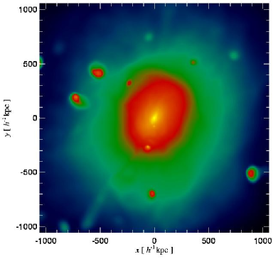
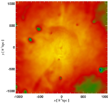
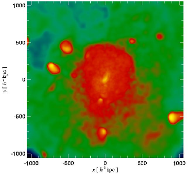
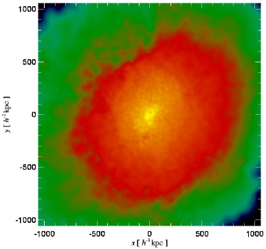
Figure 3: Projection of mass-weighted (MW) properties of gas particles contained within a sphere of radius $1\,h^{-1}\,{\rm Mpc}$ centred on the dominant cluster galaxy: hydrogen number density (top-left panel), temperature (top-right panel), iron abundance by number Fe/H referred to the solar value (bottom-left panel) and emissivity of the Fe ${\rm K}_{\alpha}$ 6.7 keV emission line normalised with the maximum mass-weighted emissivity $I_{\rm o}$ (bottom-right panel).

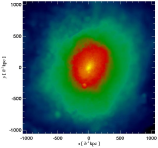
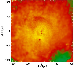
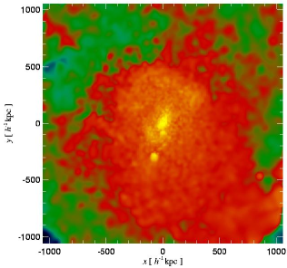
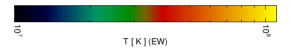
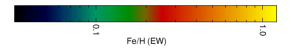
Figure 4: Projection of Fe ${\rm K}_{\alpha}$ 6.7 keV emission line-weighted (EW) properties of gas particles contained within a sphere of radius $1\,h^{-1}\,{\rm Mpc}$ centred on the dominant cluster galaxy: hydrogen number density (left panel), temperature (middle panel) and iron abundance by number Fe/H relative to the solar value (right panel).

The first step in computing line-emission weighted properties of the ICM from our simulations is to estimate the intensity of the Fe ${\rm K}_{\alpha}$ 6.7 keV emission line for each gas particle. The atomic processes involved in the generation of the emission are quite sensitive to the hydrogen volume density $n_{H}$, temperature $T$, and chemical abundances of the gas. Following the procedure performed by Furlanetto et al. (2004), we build a grid where these quantities are varied, and we compute the intensity of the emission line for each point in the grid. For this purpose we use the radiative-collisional equilibrium code CLOUDY (Ferland, 2000; Ferland et al., 2001). Given the thermodynamical conditions of the ICM, we can well approximate it as a low density hot plasma in collisional equilibrium, without being affected by an ionizing backgroud. Therefore, photoionization is discarded in the models we generate with CLOUDY.

The iron line emissivity of the gas particles that make up the ICM is obtained by interpolating the emissivities assigned to our grid of gas states, where the parameters defining the three-dimensional grid in density, temperature and iron abundances cover the range of values exhibited by the gas inside the virial radius of the cluster at $z=0$. An important detail of our chemical implementation is that we follow the evolution of the abundances of several species. Hence, instead of assuming solar metallicity for gas particles, or varying this quantity as a global parameter like in other works (e.g., Sutherland & Dopita 1993; Furlanetto et al. 2004), our grid of models depends on sets of abundances of the chemical elements considered in the semi-analytic model. As gas particles become more metal rich, the abundances of all elements increase roughly proportionally to each other. We take advantage of this feature to construct the sets of abundances characterised by the mean value of iron abundance within a certain range of values. Since we only consider the most abundant elements in our semi-analytic model, the code CLOUDY automatically gives solar values (meteroritic abundances of Grevesse & Anders (1989) with extensions by Grevesse & Noels (1993)) for the rest of the elements.

The range of values covered by the grid parameters are $1\times 10^{6}<T<1\times 10^{9}\,$ K for gas temperature, and $3.16\times 10^{-6}<n_{\rm H}<0.1\,{\rm cm}^{-3}$ for the hydrogen volume density. This last range of values is estimated from the density $\rho$ of gas particles in the N-Body/SPH simulation and from their hydrogen abundance $A_{\rm gas}^{\rm H}$ in our model. In general, this quantity ranges from the initial value of 0.76 to $\sim 0.70$, which is reached by the most metal rich particles. Iron abundances by number range from Fe/H$\sim 5\times 10^{-8}$ to $\sim 5\times 10^{-5}$, which are $\sim 1.8\times 10^{-3}$ and $\sim 1.8$ times the solar value, respectively.

We choose density spacings $\Delta\log(n_{\rm H}/{\rm cm}^{-3})=0.25$. Since emissivities are quite sensitive to temperature variations, we adopt temperature spacings of $\Delta\log(T/{\rm K})=0.1$, for $10^{7}{\rm K}<T<10^{8.5}{\rm K}$, and $\Delta\log(T/{\rm K})=0.25$ otherwise. We consider seven bins for the iron abundances with spacings $\Delta\log({\rm Fe}/{\rm H})=0.5$ from $\log({\rm Fe}/{\rm H})=-7.75$ to $-4.25$. In order to produce the whole grid of models in a systematic way, we use a user-friendly package of IDL routines that facilitates the use of the code CLOUDY (in version C96B4), called MICE (MPE IDL Cloudy Environment), developed by Henrik Spoon.

Figure 3 shows the projected mass-weighted maps of hydrogen density (top-left panel), temperature (top-right panel), iron abundance (bottom-left panel) and emissivity of the Fe ${\rm K}_{\alpha}$ 6.7 keV line normalised with the maximum mass-weighted emissivity $I_{\rm o}$ (bottom-right panel) for gas particles within a radius of $1\,h^{-1}\,{\rm Mpc}$ from the cluster centre at $z=0$. From the first three maps we can connect the iron abundances with the distributions of gas density and temperature in the ICM. We can see that those regions with high levels of chemical enrichment are associated with cool and high density areas; this fact is particularly evident in the small substructures in the outskirts of the cluster that have been recently accreted. These substructures do not produce strong X-ray emission due to their low temperature (fourth map), and the line emission map results in rather smooth maps, following mainly the coarse features of the density distribution.

Figure 4 is equivalent to Figure 3, but the Fe ${\rm K}_{\alpha}$ 6.7 keV emission-line-weighted quantities are shown instead. We can see that the denser, cooler and more metal rich substructures found in the outskirts of the mass-weighted maps of Figure 3 do not appear in the corresponding plots of Figure 4, since the intensity of the lines emitted from these regions is very low (see bottom-right panel of Figure 3).

7 Enrichment history and dynamical evolution of the ICM

In order to understand the way in which the chemical enrichment patterns characterising the intracluster gas develop, we analyse the temporal evolution of maps of the projected chemical properties of the gas and the corresponding radial abundance profiles. This allows us to evaluate the relative contribution of SNe CC and Ia to the metal enrichment, as well as to investigate the dynamical evolution of the intracluster gas which plays a fundamental role in the spatial distribution of metals.

For this purpose, we first consider gas particles lying within $500\,h^{-1}$ kpc from the cluster centre at $z=0$ and trace their properties back in time. Thus, we follow the chemical enrichment of small substructures forming at high redshift and study how they progressively become part of the cluster and contribute to establishing its final distribution of metals. Figures 5 and 6 show mass-weighted iron abundances by number relative to the sun, Fe/H (left column), the corresponding Fe ${\rm K}_{\alpha}$ 6.7 keV emission-line-weighted abundances (middle column), and the mass-weighted temperature of the gas (right column), for five different redshifts from $z\sim 1$ to $z\sim 0.1$. At each redshift, the cluster centre is defined as the centre of the most massive progenitor of the cluster at $z=0$, and the distances from it are estimated using comoving coordinates. We can see that the ICM at $z=0$ is formed by the accretion and merger of small substructures that at early times ($z\sim 1$) are spread within an extended region of radius $\sim 9\,h^{-1}$ Mpc. These gaseous building blocks are already considerably contaminated by that time, with iron abundances that reach values of ${\rm Fe}/{\rm H}\sim 0.3$.

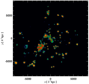
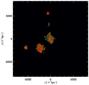
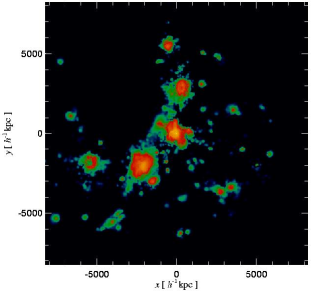
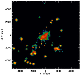
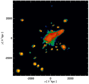
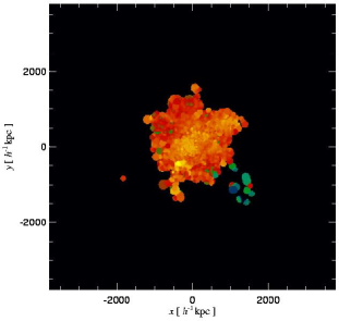
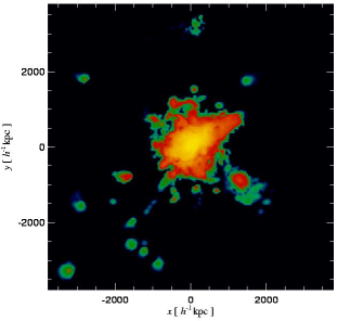
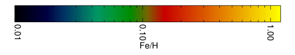
Figure 5: Evolution of iron abundance and temperature of gas particles that lie within $500\,h^{-1}$ kpc from the cluster centre at $z=0$. The plots show the projection of mass-weighted iron abundance by number relative to hydrogen, Fe/H, respect to the solar value (left column), the corresponding Fe ${\rm K}_{\alpha}$ 6.7 keV emission-line-weighted abundance (middle column), and the mass-weighted temperature of the gas (right column). We give results for three redshifts: $z\sim 1$ (lookback time of $7.8$ Gyr; first row), $z\sim 0.5$ (lookback time of $4.9$ Gyr; second row), and $z\sim 0.3$ (lookback time of $3.6$ Gyr; third row). At each refshift, the spatial coordinates are centred at the most massive progenitor of the cluster at $z=0$ and are expressed in comoving scales.

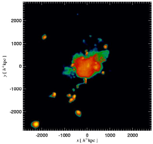
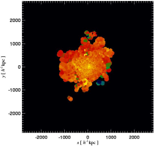
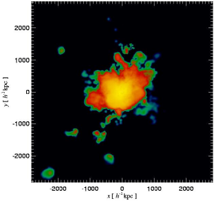
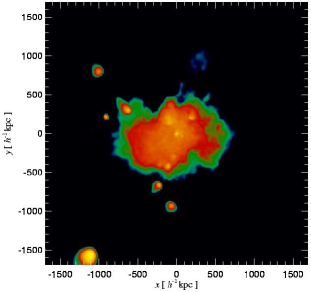
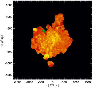
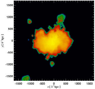
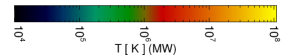
Figure 6: Same as Fig. 5, but for redshifts: $z\sim 0.2$ (lookback time of $2.4$ Gyr; first row), and $z\sim 0.1$ (lookback time of $1.2$ Gyr; second row).

From these figures, we can also infer interesting aspects about the dynamics of the contaminated gaseous clumps. Those that are at $\sim 6\,h^{-1}$ Mpc from the cluster centre at $z\sim 0.5$ needs to move at more than $\sim 1000\,{\rm km}\,{\rm s}^{-1}$ to get inside $0.5\,h^{-1}$ Mpc by $z=0$. A quantitative analysis of the dynamics of these gaseous clumps is presented in Figure 7, which shows the dependence of the velocity of gas particles with their clustercentric distances and its evolution with redshift. We identify the gas particles contained within spherical shells of $0.5\,h^{-1}$ Mpc of thickness, centred at the most massive progenitor of the cluster at $z\sim 0.5$, and estimate their mean velocities and clustercentric distances at lower redshifts. In this way, we follow the evolution of these properties as the cluster is being assembled. The different symbols denote the redshifts considered, and the lines connect the sets of gas particles defined according to their clustercentric distance at $z\sim 0.5$. There are many aspects to emphasize from this plot. At $z\sim 0.5$, gas particles have very high velocities, which range from $\sim 1300$ to $\sim 2500{\rm km}\,{\rm s}^{-1}$. The highest velocities correspond to gas particles lying between $\sim 1$ and $\sim 2\,h^{-1}$ Mpc. This is the same for redshifts $z\sim 0.3$ and $\sim 0.2$, although the velocities acquired are smaller. If we follow the evolution with redshift of gas particles lying more than $4\,h^{-1}$ Mpc at $z\sim 0.5$, we see that they are accelerated till they achieve the highest velocities at $z\sim 0.3$ and $\sim 0.2$. This occurs at a distance corresponding to the virial radius of the main progenitor, which is of the order $1\,h^{-1}$ Mpc at $z\sim 0.5$ and increases to $\sim 1.5\,h^{-1}$ Mpc at $z=0$. Thus, despite shell crossing, it is evident that the dynamics of gas particles is characterised by a general behaviour in which they are accelerated till they reach the main cluster shock radius, at a distance of the order of its virial radius, and once they have been incorporated to it they converge to the centre with velocities of $\sim 300\,{\rm km}\,{\rm s}^{-1}$. This turbulent velocity reached inside the virial radius and the infall that dominates the gas outside it are consistent with the results obtained by Sunyaev et al. (2003) based on the analysis of cluster simulations at $z=0$ (Norman & Bryan, 1999). The complex dynamics of gas particles acquired during the hierarchical formation of the structure helps to explain the way in which the metallicity profiles develop, as we discuss later in this section.

Figure 8 shows the evolution of iron and oxygen abundance profiles, which are determined for gas particles lying within the innermost comoving $1\,h^{-1}$ Mpc at $z=0$ and at each of the redshifts considered in Figures 5 and 6. The first three rows show the shape of the profiles for the combined effect of both types of SNe, and for the separate contributions of SNe Ia and CC, respectively. The plot in the last row gives the evolution of the O/Fe ratio profile resulting from the influence of the combined effect of both types of SNe. The way in which the iron and oxygen abundance profiles develop are quite similar, even though the former is mainly determined by the large amount of iron ejected by SNe Ia, while the latter is only determined by the SNe CC contribution. This fact leads to an almost flat O/Fe ratio profile at $z=0$, with a slight increasing trend at large radii. The central abundances of both Fe and O, and the almost flat O/Fe ratio show that both types of SNe contribute in a similar fashion to every part of the cluster, that is, without a preference for SNe Ia to chemically enrich the inner regions of the cluster, and for SNe CC to pollute its outskirts, as inferred from some observations (Finoguenov et al., 2001). The main change in the profiles occurs in the central region ($\la 100\,h^{-1}$ kpc) at late times by a progressive increase of the chemical abundances.

Figure 7: Mean velocities of gas particles contained within spherical shells of $0.5\,h^{-1}$ Mpc of thickness, centred at the most massive progenitor of the cluster at $z\sim 0.5$, as a function of their mean clustercentric distances. This dependence is estimated for different redshifts as denoted by the symbols. The lines connect the sets of gas particles defined according to their clustercentric distance at $z\sim 0.5$.

Figure 8: Evolution of the radial profiles of iron and oxygen abundances by number relative to hydrogen and of the profile of the O/Fe ratio, referred to the solar value. The profiles are determined for the gas contained within the innermost comoving $1\,h^{-1}$ Mpc at $z\sim 1$ (dash dot dot line), $z\sim 0.5$ (dash dot line), $z\sim 0.3$ (dashed line), $z\sim 0.2$ (dotted line), $z\sim 0.1$ (thin solid line) and $z=0$ (thick solid line). The first row shows the contributions of both types of SNe (CC and Ia) to the Fe and O abundances, while the second and third rows show the separate contributions of SNe Ia and CC, respectively. The last row presents the O/Fe abundance ratios when both types of SNe are considered.

Figure 9: Iron mass ejection rate as a function of redshift produced by SNe Ia (top panel) and SNe CC (bottom panel), contained in galaxies that lie within different distances from the cluster centre at $z=0$: the dominant cluster galaxy (at the cluster centre, thick solid line), galaxies within the spherical region with radius $0.5\,h^{-1}$ Mpc without the central galaxy (dashed line), galaxies within the spherical shells between $0.5$ and $1.\,h^{-1}$ Mpc (dash dot line), and between $1.0$ and $1.5\,h^{-1}$ Mpc (dash dot dot dot line).

The evolution of the radial abundance profiles of the main SNe Ia and CC products (iron and oxygen, respectively) from $z\sim 1$ to $z=0$, can be explained by taking into account the history of metal ejection of the cluster galaxies as well as the dynamics of the gas associated to them while galaxies are being accreted onto the cluster.

Figure 9 shows the iron mass ejection rate as a function of redshift produced by SNe Ia (top panel) and SNe CC (bottom panel) that are contained in galaxies that lie within shells of different distances from the cluster centre at $z=0$. Since we are focusing on a set of galaxies in the $z=0$ cluster, the contribution of SNe CC to the ICM chemical enrichment peaks at higher redshifts ($z\sim 5-7$) than the star formation rate of the whole simulation (see figure 1 of Ciardi et al. (2003) for a comparison of the redshift evolution of the star formation rate for field region simulations and for cluster simulations). As we have already mentioned, the SNe CC rate closely follows the star formation rate since the lifetimes of the stars involved are quite short. Instead, the ejection rate of elements produced by SNe Ia reaches a maximum at $z\sim 3-5$, due to the return time distribution resulting from the adopted model for SNe Ia explosions. The peaks in the mass ejection rates are followed by a strong decline at lower redshifts for both types of SNe, such that the ongoing chemical contamination is quite low at $z=0$. This behaviour is more pronounced for those galaxies that are nearer to the cluster centre at the present time.

Considering the accumulated mass of iron in the ICM at $z=0$, we find that SNe Ia are responsible for $\sim 75$ per cent of the iron content of the ICM. Interpretation of observed profiles of abundance ratios extends this percentage up to $\sim 80$ per cent (Gastaldello & Molendi, 2002). However, both results are quite dependent of the assumed SNe Ia model. The point that we have to emphasize is that the relative contribution of SNe CC and SNe Ia to the iron content of the cluster is already one-third at $z\sim 2$, when the accumulated iron masses provided by both sources peack. The lack of metal contribution by SNe explosions at late times from galaxies that are near the cluster centre cannot explain the increase of abundances in the inner $100\,h^{-1}$ kpc since $z\sim 0.1$, suggesting that dynamical processes are playing an important role in the developement of abundance profiles.

Figure 10 shows the evolution of mass-weighted iron abundances of gas particles contained within $1\,h^{-1}$ Mpc from the cluster centre at redshifts $z\sim 1$, $\sim 0.5$, $\sim 0.3$, $\sim 0.2$, $\sim 0.1$ and $z=0$. We clearly see from these plots that highly enriched gas clumps are already present in the outskirts of the cluster at $z\sim 0.3$ and that the iron abundance profile starts to settle down at $z\sim 0.2$. The contaminated gas clumps located near $y\sim 350\,h^{-1}$ kpc at $\sim 0.2$ and close to $y\sim 200\,h^{-1}$ kpc at $\sim 0.1$ seem to converge to the cluster centre at $z=0$ considerably increasing the iron abundance in the inner $100\,h^{-1}$ kpc. Thus, gas particles bound to the dark matter substructures of ‘halo galaxies’ (see definition in section 2.2) have been mainly enriched at early epochs, when the metal ejection rates from these galaxies were higher, and have then fallen to the inner regions of the cluster driven by the haloes of infalling galaxies. This dynamical effect is quite likely taking into account the analysis of gas dynamics based on figures 5, 6 and 7. A simple test of finding the position of the progenitor of the central galaxy at different redshifts reveals that these galaxies are at $\sim 100\,h^{-1}$ kpc at $z\sim 0.5$, reinforcing our conclusion based on gas dynamics.

The scenario of chemical enrichment considered in our model indicates that gas dynamical effects play an important role in the developement of abundance patterns. However, there are other sources of chemical elements not included in our model that may help to interprete observational results, such as intracluster stellar populations and ram-pressure stripping. There is increasing evidence of the presence of intracluster stars based on observations of diffuse light (Feldmeier 2004; Zibetti et al. 2005) and individual stars between cluster galaxies (Feldmeier 2003; Durrell et al. 2002; Gal-Yam et al. 2003). High resolution N-Body/SPH simulations are starting to yield predictions of the spatial and kinematic distributions for these stars (Willman et al. 2004; Murante et al. 2004; Sommer-Larsen, Romeo & Portinari 2005) which hold important information about the assembly history of a galaxy cluster. These numerical works show that a fraction of at least $\sim 10$ per cent of unbound stars accumulate within the cluster as a result of stripping events and infall of galaxy groups that already contain unbound stars. The impact of intracluster stars in the chemical enrichment of the ICM has been explored by Zaritsky, Gonzalez & Zabludoff (2004) by using a simple model. They demonstrate that this stellar component makes a significant contribution to the iron content of the ICM. The metal pollution due to ram-pressure stripping has been recently investigated by Schindler et al. (2005) and Domainko et al. (2005). These authors argue that the efficiency of this enrichment mechanism is higher than that of supernovae driven galactic winds, producing a centrally concentrated metal distribution in massive clusters.

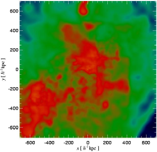
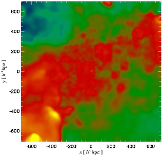
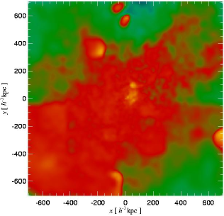
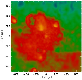
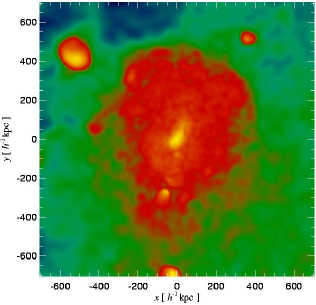
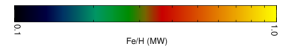
Figure 10: Evolution of iron abundance of gas particles that lie within $1\,h^{-1}$ Mpc from the cluster centre at redshifts: $z\sim 1$ (upper left panel), $z\sim 0.5$ (upper middle panel), $z\sim 0.3$ (upper right panel), $z\sim 0.2$ (lower left panel), $z\sim 0.1$ (lower middle panel) and $z=0$ (lower right panel). The plots show the projection of mass-weighted iron abundance by number relative to hydrogen, Fe/H, respect to the solar value. At each refshift, the spatial coordinates are centred at the most massive progenitor of the cluster at $z=0$ and are expressed in comoving scales.

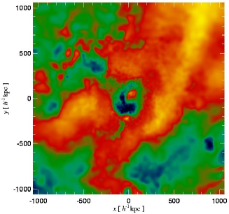
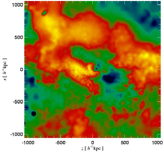
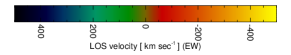
Figure 11: Projection of Fe ${\rm K}_{\alpha}$ 6.7 keV emission-line-weighted line-of-sight (LOS) velocities of gas particles contained within a sphere of radius $1\,h^{-1}\,{\rm Mpc}$ centred on the dominant cluster galaxy: $x$-$y$ projection (left panel), $y$-$z$ projection (middle panel), and $z$-$x$ projection (right panel).

8 Probing the ICM dynamics with metals

In the previous section we have showed how the complex dynamical evolution of intracluster gas influences the developement of the abundance patterns of the ICM. We now discuss the potentiality of spectroscopic observations for detecting such strong gas bulk motions, sheding light on our understanding of gas dynamics during the cluster formation.

The spatial and spectral resolution of X-ray telescope detectors onboard of present satellite missions allow the measurement of metallicity maps and of high resolution emission line spectra. The combination of these data contributes enormously to improving our knowledge about the ICM properties. For example, Fe ${\rm K}_{\alpha}$ 6.7 keV emission-line-weighted maps contain valuable information about thermodynamical and chemical properties of the intracluster gas, as discussed in Section 6. We can also learn about the kinematics of the intracluster gas and its spatial correlation with other properties from maps of emission-line-weighted line-of-sight (LOS) velocities and from Fe ${\rm K}_{\alpha}$ 6.7 keV emission line spectra generated by the gas along LOSs through the cluster.

Figure 11 shows projections of Fe ${\rm K}_{\alpha}$ 6.7 keV emission-line-weighted LOS velocities of the gas particles onto the three orthogonal planes $x$-$y$, $y$-$z$ and $z$-$x$. Velocities are relative to the cluster centre, being colour-coded such that red and yellow areas correspond to gas moving towards the observer, and green and blue represent gas receding from it. Only material contained within a sphere of radius $1\,h^{-1}\,{\rm Mpc}$ centred on the dominant galaxy of the cluster has been included. These maps exhibit steep azimuthal and radial gradients, revealing a much more complex structure than those depicted by the density, temperature and iron abundance distributions, indicating the presence of large-scale turbulent motions generated by inhomogeneous infall. This is consistent with our results on the evolution of the dynamics of gas particles based on the analysis of Figure 7. The sharp edges defined by red and green colours near the cluster centre are contact discontinuities between gas that originated in different clumps. Note that this is not a projection effect of gas particles lying far from the cluster centre. These contact discontinuities are also seen in the projection of particles well inside the cluster ($\la 50\,h^{-1}\,{\rm kpc}$).

The gradients visible in the velocity maps of Figure 11 can be as large as $\sim 1000\,{\rm km}\,{\rm s}^{-1}$ over distances of a few hundred kpc. They are of the same order of magnitude as those obtained from accurate observations of the Centaurus cluster (Abell 3526) (Dupke & Bregman, 2001). We note that this cluster is a very good candidate for this kind of studies, being one of the closest X-ray bright clusters of galaxies with an optical redshift of $0.0104$. Its core has been spatially resolved by the Chandra Observatory, using the ACIS-S detector (Sanders & Fabian, 2002), leading to temperature and abundance maps. However, there is not enough information in the spectrum to isolate spectral lines and perform accurate gas velocity measurements. This task is possible with the detector GIS on board of ASCA. The gas velocity distribution determined with this instrument (Dupke & Bregman, 2001) shows a region associated with the subcluster Cen 45, at $\sim 130\,h^{-1}\,{\rm kpc}$ from the main group Cen 30 (centred on the cD galaxy), with a radial velocity higher than the rest of the cluster by $\sim 1700\,{\rm km}\,{\rm s}^{-1}$. These radial velocity measurements obtained from X-ray observations support the optically determined velocity difference between Cen 45 and Cen 30 of $\sim 1300\,{\rm km}\,{\rm s}^{-1}$ (Stein et al., 1997).

These gradients in radial velocities are observationally detected by the Doppler shifting of the metal lines used to perform the spectral fits, which are mainly driven by the Fe ${\rm K}_{\alpha}$ complex. However, a higher spectral resolution would allow us to detect the different components in which a certain line is split due to the bulk motions of different magnitude along a line-of-sight through the cluster. Future X-ray missions promise a substantial increase in energy resolution, paving the way for the construction of a full 3-D picture of the ICM dynamics. Sunyaev et al. (2003) analyse this possibility by calculating the synthetic spectra of the Fe ${\rm K}_{\alpha}$ 6.7 keV emission line along sightlines through a simulated cluster (Norman & Bryan, 1999). They show that this emission line is split into multiple components over a range of energy $\Delta E\sim\pm 15\,{\rm eV}$, as a result of turbulent and bulk motions of the gas. They estimate that a spectral resolution of 4 eV, similar to the one planned for future missions, would be enough for the detection of dynamical features in the ICM based on emission line spectra.

Following the study made by Sunyaev et al. (2003), we analyse the way in which the special features of the gas motion that become evident in the velocity maps of Figure 11 are reflected in the Fe ${\rm K}_{\alpha}$ 6.7 keV emission line spectra generated by the gas along lines-of-sight through the cluster. The spectra are computed by dividing the sightlines in bins of width $20\,h^{-1}\,{\rm kpc}$ along directions perpendicular to the projection planes. The thermodynamical, kinematical and emission properties assigned to each bin are obtained from the 64 closest gas particles to the bin centres using the SPH smoothing technique. The energy of the iron line emitted from each bin along the sighline is Doppler shifted proportionally to the smoothed LOS velocity inferred from the gas around the bin. Combining these shifted energy values with the corresponding intensities of the line emission we obtain the iron emission line spectra along the LOS. On top of this, we consider the broadening suffered by each line due to thermal motions of the gas.

Figure 12: Fe ${\rm K}_{\alpha}$ 6.7 keV emission line spectra along three lines of sight (LOSs) on the z-axis through the simulated cluster, which is projected onto the x-y plane, and the distribution along the corresponding LOS of kinematical, thermodynamical, chemical and emissivity properties of the gas that contributes to the spectra. The upper panels show the effect of thermal broadening on the Fe emission line (thin dash-dotted curve) and the composition of thermal broadening and Doppler shift due to gas bulk motion with respect to the cluster centre (thick solid line). The maximum values of the broadened lines are used to normalise both kinds of iron emission lines, with and without Doppler shift. These panels indicate the ratio of this maximum with respect to the one corresponding to the cluster centre, $I^{\rm max}/I_{\rm o}^{\rm max}$, and the x-y position where the LOS intercepts the ICM. The five plots below each spectra show the distributions of gas properties along the corresponding sightlines: emission-line weighted LOS velocities used to generate the spectra, and mass-weighted hydrogen density $n_{\rm H}$, temperature $T$, iron abundance Fe/H, and normalised emissivity of the ${\rm K}_{\alpha}$ 6.7 keV emission line $I/I^{\rm max}$. Velocities are expressed in ${\rm km}\,{\rm s}^{-1}$, $n_{\rm H}$ in ${\rm cm}^{-3}$, $T$ in ${\rm K}$, and iron abundances are referred to the solar value. The positions along the LOSs are given with respect to the cluster centre.

Figure 13: Same as figure 12 for other set of LOSs that intercept the ICM through areas with large offset velocities present near the cluster centre as depicted by Figure 11.

Figures 12 and 13 show the resulting synthetic spectra for six LOSs along the z-axis through the x-y projection of the simulated cluster. Like in the construction of maps, the computation of the spectra only comprises gas particles within the virial radius of the cluster. Solid thick lines correspond to spectra that are affected by both Doppler shifting and thermal broadening. For comparison, we also include in each panel the iron emission line affected only by thermal broadening (dash-dotted lines). The maximum values of these last ones are used to normalise both kinds of iron emission lines, with and without Doppler shifting. The ratios of these maxima with respect to the one corresponding to the cluster centre, referred to as $I^{\rm max}/I_{\rm o}^{\rm max}$, are also given in each of the panels that show the spectra, together with the location where the LOSs intercept the ICM. Below these panels, both Figures 12 and 13 display the distribution of gas properties along the corresponding sightlines: emission-line weighted LOS velocities used to generate the spectra, and mass-weighted hydrogen density, temperature, iron abundance and normalised emissivity of the ${\rm K}_{\alpha}$ 6.7 keV emission line. These distributions allow us to see how gas components characterised by different thermodynamical and chemical properties move at different velocities, as well as which parts of the line of sight contribute most to the spectral lines.

An inspection of these distributions indicates that the gas reaches high iron abundances at high density and low temperature regions, as it is also shown by the maps of Figure 3. This situation is especially clear in the cluster core and in a subclump moving at high speed located at $\sim 500\,h^{-1}\,{\rm kpc}$ from the cluster centre, as it is evident from the first and second columns of Figure 12. The Doppler shifting and split of the emission line at the cluster core are produced by the large-scale turbulent motions of the gas, which produces a LOS velocity gradient from $\sim 200$ to $-400\,{\rm km}\,{\rm s}^{-1}$ around the middle of the sightline. This motion is reflected in the spectra because the intensity of the iron emission line is larger than $10$ per cent the central value within a radius of $\sim 100\,h^{-1}\,{\rm kpc}$ from the cluster centre. However, this intensity decays quite abruptly at larger radii and becomes undetectable (see also the mass-weighted emission map in Figure 3). For this reason, the subclump moving at $-800\,{\rm km}\,{\rm s}^{-1}$ from the cluster centre does not produce any signature in the first two Doppler shifted spectra shown. If the emissivity were higher at the location of this substructure, a peak would appear at $\sim 6,685{\rm eV}$. The second and third spectra lines in figure 12 are produced by sightlines that intercept the cluster at a distance of $100$ and $360\,h^{-1}\,{\rm kpc}$ from its centre, respectively. Note how the ratio $I^{\rm max}/I_{\rm o}^{\rm max}$ decreases as we get further from the cluster core. The second spectrum shows a clear Doppler shifting and broadening of the line, while the third one is only slightly altered with respect to the reference broadened line, in agreement with the LOS velocity distributions within the inner $\sim 100\,h^{-1}\,{\rm kpc}$.

Figure 13 presents three more synthetic spectra generated from lines of sight that intercept the cluster through areas with large offset velocities near its centre (see figure 11). The first one shows a split of the emission line in two components arising from the central velocity gradient from $\sim-200$ to $100\,{\rm km}\,{\rm s}^{-1}$. The line in the second spectrum is widely Doppler shifted as a result of high bulk motions of $\sim 500\,{\rm km}\,{\rm s}^{-1}$ in the central parts of the sightline. In the third emission line spectrum, a second component becomes apparent as a result of gas moving at $\sim-500\,{\rm km}\,{\rm s}^{-1}$. As we noted in the previous set of spectra in Figure 12, the strong gas motions of $\sim-500\,{\rm km}\,{\rm s}^{-1}$ and $\sim-700\,{\rm km}\,{\rm s}^{-1}$ occurring at $\sim 500\,h^{-1}$ Kpc from the centre of the lines of sight considered in the second and third columns are not imprinted in the corresponding spectra because of the low emissivity that characterises this region. The shifts and splits observed in all these spectra are of the order of $\sim 10-15\,{\rm eV}$. This effect is too small to be resolved by present instruments, since, for example, the spectral resolution of the EPIC pn detector for the Fe ${\rm K}_{\alpha}$ 6.7 keV emission line is 150 eV.

From this analysis we can conclude that only gas motions that produce absolute values of LOS velocities higher than $\sim 400\,{\rm km}\,{\rm s}^{-1}$ around the cluster core, where the iron line emissivity is larger than $10$ per cent the central value, could become observable by future X-ray missions through the shifting and split of the line in two components due to Doppler effects. Lower energy lines like the Fe L-blend centred around $1$ keV could be also used for the present purpose. In principle, they should show much more structure since they are strongly emitted in lower temperature gas. However, gas with this characteristic lies far from the centre of our hot cluster and the low line emissivity in these areas prevent us from getting more information from these lines than that provided by the Fe ${\rm K}_{\alpha}$ line at 6.7 keV. These lines are probably much more usefull in a lower temperature cluster.

We would like to note that the hydrodynamical simulation considered by Sunyaev et al. (2003) ignores radiative cooling, which affects the thermal structure in cluster cores, and they assume constant iron abundances to calculate the iron emission line spectra. Our simulation suffers from the first drawback as well; however, the critical advantage of our hybrid model over approaches like the one used by Sunyaev et al. (2003) is that the chemical abundances of gas particles are dynamically and consistently generated from the stars in the galaxies.

Taking into account the information supplied by LOS velocity maps and by spectra along selected sightlines, we can connect the global features of bulk motions in the gas with the multiple components in the spectra that originate as a result of these motions. Note that the latter feature can be more easily observationally detected and quantified. Thus, our results can constitute valuable help for the interpretation of observational data.

9 Summary and conclusions

We have presented an hybrid model for the chemical enrichment of the intracluster gas that allows a detailed analysis of the spatial distribution of chemical, thermodynamical and kinematical properties of the ICM. Our model combines a cosmological non-radiative hydrodynamical N-Body/SPH simulation of a cluster of galaxies, and a semi-analytic model of galaxy formation. The spatial distribution of metals in the ICM can be accounted for by the chemical enrichment of the gas particles in the underlying N-Body/SPH simulation. This enrichment results from the metals ejected by the galaxy population, which are generated by applying the semi-analytic model to the the dark matter haloes detected in the outputs of the simulation. This link between semi-analytic model results and the chemical enrichment of gas particles leads to a consistent chemical enrichment scheme for the intracluster gas, being the key ingredient to carry out the present project.

The parameters that characterise our model are chosen according to several observational constraints. The proper circulation of metals among the different baryonic components leads to a spatial distribution of chemical elements in the intracluster gas that closely resemble observed abundance patterns, as can be seen from the comparison of the radial abundance profiles with data from Tamura et al. (2004) (Figure 2). The corresponding mean iron abundance of the intracluster medium at $z=0$ is $[{\rm Fe/H}]\sim 0.28$. It has been reached with the contribution of SNe Ia that provide $\sim 75$ per cent of the total ICM iron content at $z=0$. While this percentage is quite dependent on the parameters that characterise the chemical model implemented, what reflects the circulation of metals is the fraction of elements from different sources that end up in the ICM as opposed to in stars. The fraction of iron originated in SNe Ia that is contained in the ICM is $\sim 0.78$ while that locked in the stars of cluster galaxies is $\sim 0.21$. These fractions are slightly different for the iron ejected by SNe II, being $\sim 0.72$ and $\sim 0.28$ for hot gas and stars, respectively. The increment of the proportion of SNe II products in stars reflects the relative time-scales for star formation and metal pollution by different types of supernovae.

After showing that our model reproduces reasonably well the distribution of metals in the ICM at $z=0$, we analyse the evolution of chemical and dynamical properties of the intracluster gas in order to understand the physical processes involved in the determination of its final abundance patterns. The aim of this study is also to provide hints that helps in gaining information about the characteristics of gas bulk motions from spectroscopic observations. We analyse the rich information provided by our hybrid model in three ways,

1. by constructing radial abundance profiles of the ICM,

2. by building projected mass-weighted and Fe ${\rm K}_{\alpha}$ 6.7 keV emission-line-weighted maps of chemical, thermodynamical and kinematical properties of the diffuse gas,

3. and by calculating synthetic spectra of the Fe ${\rm K}_{\alpha}$ 6.7 keV emission line along sightlines through the simulated cluster.

The spatial distribution of chemical elements leads to radial abundance profiles with negative gradients, irrespective of the type of source from where they originated. The central enhancement of the Fe and O abundance profiles and the flat profile of the O/Fe ratio support the notion that the intracluster gas is polluted in the same way by both types of SNe. From the analysis of the evolution of these radial abundance profiles and the projected mass-weighted iron abundance of gas particles at different redshifts we find that a high level of enrichment of the ICM is already reached at $z\sim 1$. Despite the delay time for the ejection of metals inherent to SNe Ia, the contribution of both types of SNe to the ICM chemical enrichment peaks at $z\sim 2$.

The lack of evolution of mean iron abundances up to $z\sim 1$ is in agreement with observations of distant clusters (Tozzi et al., 2003). However, the final abundance profile of the cluster gets steeper within the inner $\sim 100h^{-1}$ Kpc during the last Gyr (see the increments between $z\sim 0.1$ and $z=0$ in Figure 8). This cannot be accounted for the metal production of the cluster galaxies. The peaks in the rates of the ejected iron mass from these galaxies are followed by a strong decline towards lower redshifts for both types of SNe, such that the ongoing chemical contamination at $z=0$ is quite low; this behaviour is more pronounced for galaxies that are nearer to the cluster centre at the present time. The combination of all these results indicates that the enhancement of central abundances produced at low redshift cannot be explained by metals ejected during this time interval from galaxies that lie close to the cluster centre. Indeed, galaxies within a sphere of radius $500\,h^{-1}\,{\rm kpc}$ centred on the dominant cluster galaxy do not contribute to the metal enrichment at recent epochs. Instead, a scenario appears favoured in which gas particles are primarily enriched at high redshifts, and are subsequently driven to the cluster centre by bulk motions in the intracluster gas. Hence, the main cause that contribute to this central abundances enhancement is the dynamical evolution of gas particles during the cluster formation.

Gas particles develop very high velocities ranging from $\sim 1300$ to $\sim 2500\,{\rm km}\,{\rm s}^{-1}$ when they are farther than $\sim 1\,h^{-1}$ Mpc from the cluster centre at $z>0.2$. Once these high velocity gas clumps cross this typical cluster shock radius, which correspond approximately to the virial radius of the most massive progenitor of the cluster at these redshifts, they slow down ending up within the inner $\sim 500h^{-1}$ Kpc of the cluster at $z=0$. The inhomogeneous gas infall produces contact discontinuities that are manifested as sharp edges in the emission-line-weighted line-of-sight velocity maps. These maps provide useful information about the gas dynamics in the ICM and its dependence on spatial position within the cluster. They reveal a quite complex structure of the gas dynamics, including the presence of strong radial and azimuthal gradients with values as large as $\sim 1000\,{\rm km}\,{\rm s}^{-1}$. Gradients of this magnitude are also seen in velocity distributions along sightlines through the cluster centre. Doppler shifting and broadening suffered by the Fe ${\rm K}_{\alpha}$ 6.7 keV emission line along sightlines could be used to probe these gas bulk motions when they are produced within an area characterised by high iron line emissivity. Velocities of $\sim 400\,{\rm km}\,{\rm s}^{-1}$, typically found within a radius of $100\,h^{-1}\,{\rm kpc}$ from the cluster core, produce Doppler shifts of the line of the order of $\sim 10-15\,{\rm eV}$. The line can be split in multiple components depending on the structure of the velocity field. We find that the higher velocities reached by the intracluster gas beyond $500\,h^{-1}\,{\rm kpc}$, or those aquired by infalling subclumps located at such large distances from the cluster centre do not produce a detectable signature in the spectral lines because of the rather low iron line emissivity in the outskirts of the cluster.

The combination of all these results strongly supports the fact that abundance patterns of the ICM are the result of gas mixing because of hydrodynamical processes during cluster formation, being a considerable amount of the gas mainly enriched at high redshifts, before the cluster have time to virialise. The central enhancement of Fe and O abundance profiles might be considered as produced by a particular situation taking place in our simulation, in which two big highly enriched gas subclumps converge at the cluster centre at the present epoch. However, this kind of behaviuor is consistent with the hierarchical formation scenario, in which accretion and merging of substructures constitute the main processes driving the formation and evolution of clusters of galaxies. Thus, the specific shape of metallicity profiles might well be a consequence of the combination of two time-scales, one related to the metal production of galaxy clusters and the other to the metal mixing. In this last case, both the effect of gas dynamics, galaxy mergers and the efficiency in the diffusion of metals due to energetic and chemical feedback associated with the star formation process play an important role. Other enrichment processes not taken into account in our model, such as metal pollution by intracluster stars and ram-pressure stripping, may contribute significantly to recover the observed abundance patterns reinforcing the effect of gas dynamics discussed here.

Our analysis techniques in this study yield a 3-D picture of the chemical and dynamical properties of the ICM. The information about the latter can be extracted from the metal content of the intracluster gas. Our results show that gas bulk motions are imprinted in the shape of X-ray lines of heavy ions. Since thermal broadening is small, these features could be detected with the high-resolution spectrographs of future X-ray missions (CONSTELLATION-X and XEUS). Such observations should be very important in determining the physical processes involved in the formation and evolution of galaxy clusters, contributing with clues that allow us to verify the enrichment scenario inferred from our model in which gas dynamics has a crucial effect.

Finally, even though all the processes considered in our hybrid model are tuned to satisfy numerous observational constraints, the implied global level of iron enrichment we find is on the low side of the generally accepted observed range, which is around one-third the solar value. This may in part be due to the uncertainties in the stellar yields and to our poor knowledge of the strength and nature of the feedback processes involved, but could also point to a systematic problem with the observational estimates. Our model so far only accounts for the effect of SNe driven outflows, but it should be possible to include other sources of feedback, like those from AGN, as well. This is left for future work, and may perhaps provide a solution to some of the puzzles still present in understanding the observed cluster metallicities.

References

- Aguerri et al. (2005) Aguerri J.A.L., Gerhard O.E., Arnaboldi M., Napolitano N.R., Castro-Rodriguez N., Freeman K. C., 2005, AJ, 129, 2585
- Asplund et al. (2005) Asplund M., Grevesse N., Sauval A. J., 2005, in Cosmic Abundances as Records of Stellar Evolution and Nucleosynthesis, ed. T.G. Barnes III, F.N. Bash, ASP Conference Series, 336, 25
- Baumgartner et al. (2005) Baumgartner W.H., Loewenstein M., Horner D.J., Mushotzky R.F., 2005, ApJ, 620, 680
- Binney & Tremaine (1987) Binney J., Tremaine S., 1987, Galactic Dynamics, Princeton University Press
- Bruzual & Charlot (1993) Bruzual G., Charlot S., 1993, ApJ, 367, 126
- Cappellaro et al. (1999) Cappellaro E., Evans R., Turatto M., 1999, A&A, 351, 459
- Carlberg et al. (1996) Carlberg R.G., Yee H.K.C., Ellingston E., Abraham R., Gravel P., 1996, ApJ, 462, 32
- Ciardi et al. (2003) Ciardi B., Stoehr F., White S. D. M., 2003, MNRAS, 343, 1101
- Cole et al. (2000) Cole S., Lacey C.G., Baugh C.M., Frenk C.S., 2000, MNRAS, 319, 168
- Dahlen et al. (2004) Dalhen T., Strolger L.-G., Riess A.G., Mobasher B., Chary R.-R., Conselice C.J., Ferguson H.C., Fruchter A.S., et. al., 2004, ApJ, 613, 189
- De Grandi & Molendi (2001) De Grandi S., Molendi S., 2001, ApJ, 551, 153
- De Grandi et al. (2003) De Grandi S., Ettori S., Longhetti M., Molendi S., 2003, A&A, 419, 7
- De Lucia et al. (2004) De Lucia G., Kauffmann G., White S.D.M., 2004, MNRAS, 349, 1101 (DL04)
- Domainko et al. (2005) Domainko W., Mair M., Kapferer W., van Kampen E., Kronberger T., Schindler S., Kimeswenger S., Ruffert M, et al., 2005, A&A, preprint (astro-ph/0507605)
- Dupke & Bregman (2001) Dupke R.A., Bregman J. N., 2001, ApJ, 562, 266
- Durrell et al. (2002) Durrell P.R., Ciardullo R., Feldmeier J.J., Jacoby G.H., Sigurdsson S., 2002, ApJ, 570, 119
- Ettori et al. (2001) Ettori S., Allen S.W., Fabian A.C., 2001, MNRAS, 322, 187
- Evrard (1990) Evrard A.E., 1990, ApJ, 363, 349
- Feldmeier (2003) Feldmeier J.J., Ciardullo R., Jacoby G.H., Durrell P.R., 2003, ApJS, 145, 65
- Feldmeier (2004) Feldmeier J.J., Mihos J.C., Morrison H.L., Harding P., Kaib N., Dubinski J., 2004, ApJ, 609, 617
- Ferland (2000) Ferland G.J., 2000, in revista Mexicana de Astronomia y Astrofísica conference Series, 153
- Ferland et al. (2001) Ferland G.J., 2001, Hazy, A Brief Introduction to Cloudy 96 (http:///www.pa.uky.edu gary/cloudy/)
- Finoguenov et al. (2000) Finoguenov A., David L.P., Ponman T.J., 2000, ApJ, 544, 188
- Finoguenov et al. (2001) Finoguenov A., Arnaud M., David L.P., 2001, ApJ, 555, 191
- Finoguenov et al. (2002) Finoguenov A., Matsushita K., Böhringer H., Ikebe Y., Arnaud M., 2002, A&A, 381, 21
- Frenk et al. (1999) Frenk C.S., White S.D.M., Bode P., Bond J.R., Bryan G.L., Cen R., Couchman H.M.P., Evrard A.E., Gnedin N., Jenkins A., et al., 1999, ApJ, 525, 554
- Fukazawa et al. (1998) Fukazawa Y., Makishima K., Tamura T., Ezawa H., Xu H., Ikebe Y., Kikuchi K., Ohashi T., 1998, PASJ, 50, 187
- Fukazawa, Kawano & Kawashima (2004) Fukazawa Y., Kawano N., Kawashima K., 2004, ApJ, 606, L109
- Furlanetto et al. (2004) Furlanetto S.R., Schaye J., Springel V., Hernquist L., 2004, ApJ, 606, 221
- Gal-Yam et al. (2003) Gal-Yam A., Maoz D., Guhathakurta P., Filippenko A.V., 2003, AJ, 125, 1087
- Gastaldello & Molendi (2002) Gastaldello F., Molendi S., 2002, ApJ, 572, 160
- Gibson, Loewenstein & Mushotzky (1997) Gibson B.K., Loewenstein M., Mushotzky R.F., 1997, MNRAS, 290, 623
- Girardi (2000) Girardi M, Borgani S., Giuricin G., Mardirossian F., Mezzetti M., 2000, ApJ, 530, 62
- Greggio & Renzini (1983) Greggio L., Renzini A., 1983, A&A, 118, 217
- Greggio (2005) Greggio L., 2005, A&A, 441, 1055
- Grevesse & Anders (1989) Grevesse N., Anders E., 1989, Cosmic Abundances of Matter, AIP Conference Proceedings 183, p. 1, Ed. C.J. Waddington (New York: AIP)
- Grevesse & Noels (1993) Grevesse N., Anders A., 1993, in Origin & Evolution of the Elements, ed. N. Prantzos, E. Vangioni-Flam, M. Casse, p. 15 (Cambridge: Cambrigde Univ. Press)
- Hachisu, Kato & Nomoto (1999) Hachisu I., Kato M., Nomoto K., 1999, ApJ, 522, 487
- Hardin et al. (2000) Hardin D., Afonso C., Alard C., Albert J.N., Amadon A., Andersen J., Ansari R., Aubourg E., Bareyre P., Bauer F., et al., 2000, A&A, 362, 419
- Iwamoto et al. (1999) Iwamoto K., Brachwitz F., Nomoto K., Kishimoto N., Umeda H., Hix W.H., Thielemann F.-K., 1999, ApJS, 125, 439
- Humphrey & Buote (2005) Humphrey P.J., Buote D.A., 2005, ApJ, preprint (astro-ph/0504008)
- Kapferer et al. (2005) Kapferer W., Ferrari C., Domainko W., Mair M., Kronberger T., Schindler S., Kimeswenger S., van Kampen E., et al., 2005, A&A, preprint (astro-ph/0508107)
- Kauffmann & Charlot (1998) Kauffmann G., Charlot S., 1998, MNRAS, 294, 705
- Kauffmann et al. (1999) Kauffmann G., Colberg J.M., Diaferio A., White S.D.M., 1999, MNRAS, 303, 188
- Kent & Gunn (1983) Kent S.M., Gunn J.E., 1982, AJ, 88, 697
- Lia, Portinari & Carraro (2002) Lia C., Portinari L., Carraro G., 2002, MNRAS, 330, 821
- Lin et al. (2003) Lin Y.-T., Mohr J.J., Standford S.A., 2003, ApJ, 591, 749
- Loewenstein (2001) Loewenstein M., 2001, ApJ, 557, L573
- Madgwick et al. (2003) Madgwick D.S., Hewett P.C., Mortlock D.J., Wang L., 2003, ApJL, 599, L33
- Marigo (2001) Marigo P., 2001, A&A, 194, 217
- Matsushita, Finoguenov & Böhringer (2003) Matsushita K., Finoguenov A., Böhringer H., 2003, A&A, 401, 443
- Moretti et al. (2003) Moretti A., Portinari L., Chiosi C., 2003, A&A, 408, 431
- Mori & Burkert (2000) Mori M., Burkert A., 2000, ApJ, 538, 559
- Murante et al. (2004) Murante G., Arnaboldi M., Gerhard O., Borgani S., Cheng L.M., Diaferio A., Dolag K., Moscardini L., Tormen G., Tornatore L., Tozzi P., 2004, ApJ, 607, L83
- Nagashima et al. (2005) Nagashima M., Lacey C., Baugh C.M., Frenk C.C., 2005, MNRAS, 358, 1247
- Norman & Bryan (1999) Norman M.L., Bryan G.L., 1999, in Numerical Astrophysics 1998, eds. S. Miyama, K. Tomisaka, Astrophysics and Space Science Library, vol. 240, (Kluwer, Boston), 106
- Padovani & Matteucci (1993) Padovani P., Matteucci F., 1993, ApJ, 416,26
- Pain et al. (1996) Pain R., Hook I.M., Deustua S., Gabi S., Goldhaber G., Groom D., Kim A.G., Kim M.Y., Lee J.C., Pennypacker C.R., et al., 1996, ApJ, 473, 356
- Pain et al. (2002) Pain R., Fabbro S., Sullivan M., Ellis R.S., Aldering G., Astier P., Deustua S.E., Fruchter A.S., Goldhaber G., Goobar A., et al., 2002, ApJ, 577, 120
- Portinari et al. (1998) Portinari L., Chiosi C., Bressan A., 1998, A&A, 334, 505
- Renzini (1993) Renzini A., 1993, ApJ, 419, 52
- Renzini (1997) Renzini A., 1997, ApJ, 488, 35
- Renzini (2003) Renzini A., 2003, in Clusters of Galaxies: Probes of Cosmologicas Structure and Galaxy Evolution, ed. J.S. Mulchaey, A. Dressler, A. Oemler, as part of the Carnegie Observatories Astrophysics Series, (Cambridge: Cambridge Univ. Press), 261
- Ruiz-Lapuente & Canal (1998) Ruiz-Lapuente P., Canal R. 1998, ApJL, 497, L57
- Sanders & Fabian (2002) Sanders J.S., Fabian A.C., 2002, MNRAS, 331, 273
- Sommer-Larsen, Romeo & Portinari (2005) Sommer-Larsen J. Romeo A.D., Portinari L., 2005, MNRAS, 357, 478
- Sanders et al. (2004) Sanders J.S., Fabian A.C., Allen S.W., Schmidt R.W., 2004, MNRAS, 349, 952
- Sarazin (1986) Sarazin C.L., 1986, Rev. Mod. Phys., 58, 1
- Schindler et al. (2005) Schindler S., Kapferer W., Domainko W., Mair M., van Kampen E., Kronberger T., Kimeswerger S., Ruffert M., Mangete O., Breitschwerdt D., 2005, A&A, 435, L25
- Schmidt et al. (2002) Schmidt R.W., Fabian A.C., Sanders J.S., 2002, MNRAS, 337, 71
- Springel, Yoshida & White (2001) Springel V., Yoshida N., White S.D.M., 2001, New Astronomy, 79, 117
- Springel et al. (2001) Springel V., White S.D.M., Tormen G., Kauffmann G., 2001, MNRAS, 238, 726
- Springel & Hernquist (2003) Springel V., Hernquist L. 2003, MNRAS, 339, 312
- Springel (2005) Springel V., 2005, MNRAS, MNRAS, 364, 1105
- Somerville et al. (2001) Somerville R.S., Primack J.R., Faber S.M., 2001, MNRAS, 320, 504
- Stein et al. (1997) Stein P., Jerjen H., Federspiel M., 1997, A&A, 327, 952
- Strolger et al. (2004) Strolger L.-G., Riess A.G, Dahlen T., Livio M, Panagia N., Challis P. Tonry J.L., Filippenko, A. V., et al., 2004, ApJ, 613, 200
- Sunyaev et al. (2003) Sunyaev R.A., Norman M.L., Bryan G.L., 2003, Astronomy Letters, 29, 783
- Sutherland & Dopita (1993) Sutherland R.S., Dopita M.A., 1993, ApJS, 88, 253
- Tamura et al. (2004) Tamura T., Kaastra J.S., Herder J.W.A.den., Bleeker J.A.M., Peterson J.R., 2004, A&A, 420, 135
- Tonry et al. (2003) Tonry J.L., Schmidt B.P., Barris B., Candia P., Challis P.; Clocchiatti A., Coil A.L., Filippenko A.V., et al. 2003, ApJ, 594, 1
- Tornatore et al. (2004) Tornatore L., Borgani S., Matteucci F., Recchi S., Tozzi P., 2004, MNRAS, 349, L19
- Tozzi et al. (2003) Tozzi P., Rosati P., Ettori S., Borgani S., Mainieri V., Norman C., 2003, ApJ, 593, 705
- Tutukov & Yungelson (1994) Tutukov A. V., Yungelson L. R., 1994, MNRAS, 268, 871
- Valdarnini (2002) Valdarnini R. 2002, ApJ, 567,741
- Valdarnini (2003) Valdarnini R. 2003, MNRAS, 339, 1117
- White (1991) White R., 1991, ApJ, 367, 69
- Willman et al. (2004) Willman B., Governato F., Wadsley J., Quinn T., 2004, MNRAS, 355, 159
- Woosley & Weaver (1995) Woosley S.E., Weaver T.A., 1995, ApJS, 101, 181
- Yoshii, Tsujimoto & Nomoto (1996) Yoshii Y., Tsujimoto T., Nomoto K. 1996, ApJ, 462, 266
- Zaritsky, Gonzalez & Zabludoff (2004) Zaritsky D., Gonzalez A.H., Zabludoff A.I., 2004, ApJ, 613, L93
- Zibetti et al. (2005) Zibetti S., White S.D.M., Schneider D.P., Brinkmann J., 2005, MNRAS, 358, 949