Cosmological Radiative Transfer Codes Comparison Project I: The Static Density Field Tests

Abstract

Radiative transfer simulations are now at the forefront of numerical astrophysics. They are becoming crucial for an increasing number of astrophysical and cosmological problems; at the same time their computational cost has come to the reach of currently available computational power. Further progress is retarded by the considerable number of different algorithms (including various flavours of ray-tracing and moment schemes) developed, which makes the selection of the most suitable technique for a given problem a non-trivial task. Assessing the validity ranges, accuracy and performances of these schemes is the main aim of this paper, for which we have compared 11 independent RT codes on 5 test problems: (0) basic physics, (1) isothermal H II region expansion and (2) H II region expansion with evolving temperature, (3) I-front trapping and shadowing by a dense clump, (4) multiple sources in a cosmological density field. The outputs of these tests have been compared and differences analyzed. The agreement between the various codes is satisfactory although not perfect. The main source of discrepancy appears to reside in the multi-frequency treatment approach, resulting in different thicknesses of the ionized-neutral transition regions and the temperature structure. The present results and tests represent the most complete benchmark available for the development of new codes and improvement of existing ones. To this aim all test inputs and outputs are made publicly available in digital form.

1 Introduction

Numerous physical problems require a detailed understanding of radiative transfer (RT) of photons in different environments, ranging from intergalactic and interstellar medium to stellar or planetary atmospheres. In particular, a number of problems of cosmological interest cannot be solved without incorporating RT calculations, e.g. modeling and understanding of the Ly$\alpha$ forest, absorption lines in spectra of high-z quasars, radiative feedback effects, the reionization of the intergalactic medium (IGM) and star formation, just to mention a few (see e.g. Ciardi & Ferrara 2005, for a recent review on some of these topics). In many of these situations, the physical conditions are such that the gas in which photons propagate is optically thick; also, the geometry of the problem often is quite complex. As a consequence, approaches relying on optically thin or geometrical approximations yield unsatisfactory (and sometimes incorrect) results.

The RT equation in 3D space has seven (three spatial, two angular, one frequency, one time) dimensions. Although in specific cases certain kinds of symmetry or approximations can be exploited, leading to a partial simplification, most problems of astrophysical and cosmological interest remain very complex. For this reason, although the basic physics involved is well understood, the detailed solution of the complete radiative transfer equation is presently beyond the available computational capabilities. In addition, the technical implementation of the RT equation in numerical codes is a very young and immature subject in astrophysics.

RT approaches have been attempted in the past to study specific problems as the light curves of supernovae, radiation from proto-stellar and active galactic nuclei accretion disks, line radiation from collapsing molecular clouds, continuum photon escape from galaxies and the effects of dust obscuration in galaxies. Typically, either the low dimensionality of these approaches or the simplified physics allowed a numerical treatment that resulted in a sufficiently low computational cost given the available machines. As this last constraint has become less demanding, the number and type of desirable applications has expanded extremely rapidly, particularly spreading to galaxy formation and cosmology fields.

Following this wave of excitement, several groups then attacked the problem from a variety of perspectives by using completely different, independent, and dedicated numerical algorithms. It was immediately clear that the validation and assessment of the various codes was crucial in order not to waste (always) limited computational and human resources. At that point the community faced the problem that, in contrast with e.g. gas-dynamic studies, very few simple radiative transfer problems admit exact analytical solutions that could be used as benchmarks. Just a few years ago only a few RT codes were available and these were still mostly in the testing/optimization phase, and therefore lacking the necessary degree of stability required to isolate truly scientific results from uncertainties due to internal programming bugs. In the last few years the subject has rapidly changed. Not only has the reliability of existing codes matured, a new crop of codes based on novel techniques has been developed, making a comparison of them timely. The time is now ripe to do this comparison project in a fairly complete and meaningful form and this paper presents the detailed outcome of our effort.

The aim of the present comparison is to determine the type of problems the codes are (un)able to solve, to understand the origin of the differences inevitably found in the results, to stimulate improvements and further developments of the existing codes and, finally, to serve as a benchmark to testing future ones. We therefore invite interested RT researchers to make use of our results, including tests descriptions, input and output data, all of which can be found in digital form at the project website http://www.mpa-garching.mpg.de/tsu3/. At this stage our interest is not focused on the performances of the codes in terms of speed and optimization.

This project is a collaboration of most of the community and includes a wide range of different methods (e.g. various versions of ray-tracing, as well as moment schemes), some of which have already been applied to study a variety of astrophysical and cosmological problems. The comparison is made among 11 independent codes, each of which is described concisely in § 2 (and more extensively in the corresponding methodology paper, whenever available). We would like to emphasize that the interaction among the various participating groups has been characterized by a very constructive and scientifically honest attitude, and resulted in many improvements of the codes.

Here we present the results from a set of tests on fixed density fields, both homogeneous and inhomogeneous, which verify the radiative transfer methods themselves. In a follow-up paper we plan to discuss the direct coupling to gas-dynamics and compare the results on a set of several radiative hydrodynamics problems.

2 The Codes

In this section we briefly describe the eleven radiative transfer codes which are taking part in this comparison project. The descriptions point to the more detailed methodology papers whenever available. All the codes, their names, authors and current features are summarized in Table 1.

Table 1: Participating codes and their current features.

Code (Authors)	Grid	Parallelization	gasdynamics	Helium	Rec. radiation
$C^{2}$-Ray (G. Mellema, I. Iliev, P. Shapiro, M. Alvarez)	fixed/AMR	shared	yes	no	no
OTVET (N. Gnedin, T. Abel)	fixed	shared	yes	yes	yes
CRASH (A. Maselli, A. Ferrara, B. Ciardi)	fixed	no	no	yes	yes
RSPH (H. Susa, M. Umemura)	no grid, particle-based	distributed	yes	no	no
ART (T. Nakamoto, H. Susa, K. Hiroi, M. Umemura)	fixed	distributed	no	no	yes
FTTE (A. Razoumov)	fixed/AMR	no	yes	yes	yes
SimpleX (J. Ritzerveld, V. Icke, E.-J. Rijkhorst)	unstructured	no	no	no	yes
Zeus-MP (D. Whalen, M. Norman)	fixed	distributed	yes	no	no
FLASH-HC (E.-J. Rijkhorst, T. Plewa, A. Dubey, G. Mellema)	fixed/AMR	distributed	yes	no	no
IFT (M. Alvarez, P. Shapiro)	fixed/AMR	no	no	no	no
Coral (I. Iliev, A. Raga, G. Mellema, P. Shapiro)	AMR	no	yes	yes	no

2.1 $C^{2}$-Ray: Photon-conserving transport of ionizing radiation (G. Mellema, I. Iliev, P. Shapiro, M. Alvarez)

C²-Ray is a grid-based short characteristics ray-tracing code which is photon-conserving and causally traces the rays away from the ionizing sources up to each cell. Explicit photon-conservation is assured by taking a finite-volume approach when calculating the photoionization rates, and by using time-averaged optical depths. The latter property allows for integration time steps much larger than the ionization time scale, which leads to a considerable speed-up of the calculation and facilitates the coupling of our code to gasdynamic evolution. The code is described and tested in detail in Mellema et al. (2006a).

The frequency dependence of the photoionization rates and the photoionization heating rates is dealt with by using frequency-integrated rates, stored as functions of the optical depth at the ionization threshold. In its current version the code includes only hydrogen and does not include the effects of helium, although they could be added in a relatively straightforward way.

The transfer calculation is done using short characteristics, where the optical depth is calculated by interpolating values of grid cells lying closer to the source. Because of the causal nature of the ray-tracing, the calculation cannot easily be parallelized through domain decomposition. However, using OpenMP the code is efficiently parallelized over the sources. The code is currently used for large-scale simulations of cosmic reionization and its observability (Iliev et al. 2005b; Mellema et al. 2006b) on grid sizes up to $406^{3}$ and up to more than $10^{5}$ ionizing sources.

There are 1D, 2D and 3D versions of the code available. It was developed to be directly coupled with hydrodynamics calculations. The large time steps allowed for the radiative transfer enable the use of the hydrodynamic time step for evolving the combined system. The first gasdynamic application of our code is presented in Mellema et al. (2005).

2.2 OTVET: Optically-Thin Variable Eddington Tensor Code (N. Gnedin, T. Abel)

The Optically Thin Variable Eddington Tensor (OTVET) approximation (Gnedin & Abel 2001) is based on the moment formulation of the radiative transfer equation:

$${a\over c}{\partial E_{\nu}\over\partial t}+{\partial F^{i}_{\nu}\over\partial x^{i}} = -\hat{\kappa}_{\nu}E_{\nu}+S_{\nu},$$

$${a\over c}{\partial F^{j}_{\nu}\over\partial t}+{\partial\over\partial x^{i}}E_{\nu}h^{ij}_{\nu} = -\hat{\kappa}_{\nu}F^{j}_{\nu},$$ (1)

where $E_{\nu}$ and $F^{j}_{\nu}$ are the energy density and the flux of radiation respectively, $\kappa_{\nu}$ is the absorption coefficient, $S_{\nu}$ is the source function, and $h^{ij}_{\nu}$ is a unit trace tensor normally called the Eddington tensor.

It is important to underscore that the source function $S_{\nu}(\vec{x})$ is considered to be an arbitrary function of position, so that it may contain both the delta-function contributions from any number of individual point sources and the smoothly varying contributions from the diffuse sources.

Equations (1) form an open system of two partial differential equations, because the Eddington tensor can not be determined from them. In the OTVET approximation the Eddington tensor is computed from all sources of radiation as if they were optically thin, $h_{\nu}^{ij}={P_{\nu}^{ij}/{\rm Tr\,}P_{\nu}^{ij}}$, where

$$P_{\nu}^{ij}=\int d^{3}x_{1}\rho_{*}(\vec{x}_{1}){(x^{i}-x_{1}^{i})(x^{j}-x_{1}^{j})\over(\vec{x}-\vec{x}_{1})^{4}},$$

where $\rho_{*}$ is the mass density of the sources e.g. stars.

Thus, the OTVET approximation conserves the number density of photons (in the absence of absorption) and the flux, but may introduce an error in the direction of the flux propagation. It can be shown rigorously that the OTVET approximation is exact for a single point-like source and for uniformly distributed sources, but is not exact in other cases.

While it is difficult to prove rigorously, it appears that the largest error is introduced for the case of two sources, one much stronger than the other. In that case the H II region around the strong source is modeled highly precisely, but the shape of the H II region around the weaker source (before the two H II regions merge) becomes ellipsoidal with the deviation from the spherical symmetry never exceeding 17% (1/6) in any direction.

2.3 CRASH: Cosmological RAdiative transfer Scheme for Hydrodynamics (A. Maselli, A. Ferrara, B. Ciardi)

CRASH is a 3D ray-tracing radiative-transfer code based on the Monte Carlo (MC) technique for sampling distribution functions. The grid-based algorithm follows the propagation of the ionizing radiation through an arbitrary H/He static density field and calculates the time-evolving temperature and ionization structure of the gas.

The MC approach to RT requires that the radiation field is discretized into photon packets. The radiation field is thus reproduced by emitting packets, according to the configuration under analysis, and by following their propagation accounting for the opacity of the gas. For each emitted photon packet, the emission location, frequency and propagation direction are determined by randomly sampling the appropriate probability distribution functions (PDFs), which are assigned as initial conditions. It is possible to include an arbitrary number of point/extended sources and/or diffuse background radiation in a single simulation. This approach thus allows a straightforward and self-consistent treatment of the diffuse radiation produced by H/He recombinations in the ionized gas.

The relevant radiation-matter interactions are accounted for during the photon packet’s propagation. At each cell crossed, each packet deposits a fraction of its photon content according to the cell’s opacity which determines the absorption probability. Once the number of photons absorbed in the cell is calculated, we find the effect on the temperature and on the ionization state of the gas, by solving the discretized non-equilibrium chemistry and energy equations. Recombinations, collisional ionizations and cooling are treated as continuous processes.

The detailed description of the CRASH implementation is given in Ciardi et al. (2001) and Maselli et al. (2003), and an improved algorithm for dealing with a background diffuse ionizing radiation is described in Maselli & Ferrara (2005). The tests described in this paper have been performed using the most updated version of the code (Maselli et al. 2003).

The code has been primarily developed to study a number of cosmological problems, such as hydrogen and helium reionization, the physical state of the Ly$\alpha$ forest, the escape fraction of Lyman continuum photons from galaxies, the diffuse Ly$\alpha$ emission from recombining gas. However, its flexibility allows applications that could be relevant to a wide range of astrophysical problems. The code architecture is sufficiently simple that additional physics can be easily added using the algorithms already implemented. For example, dust absorption/re-emission can be included with minimum effort; molecular opacity and line emission, although more complicated, do not represent a particular challenge given the numerical scheme adopted. Obviously, were such processes added, the computational time could become so long that parallelization would be necessary. This would be required also when CRASH will be coupled to a hydrodynamical code to study the feedback of photo-processes onto the (thermo-)dynamics of the system.

2.4 RSPH: SPH coupled with radiative transfer (H. Susa, M. Umemura)

The Radiation-SPH scheme is designed to investigate the formation and evolution of the first generation objects at $z\lower 2.15277pt\hbox{$\;\buildrel>\over{\sim}\;$}10$ (Susa 2006), where the radiative feedback from various sources play important roles. The code can compute the fraction of chemical species e, H⁺, H, H^-, H₂, and H${}_{2}^{+}$ by fully implicit time integration. It also can deal with multiple sources of ionizing radiation, as well as the radiation in the Lyman-Werner band.

Hydrodynamics is calculated by the Smoothed Particle Hydrodynamics (SPH) method. We use the version of SPH by Umemura (1993) with the modification by Steinmetz & Mueller (1993), and we also adopt the particle resizing formalism by Thacker et al. (2000). In the present version, we do not use the entropy formalism.

The non-equilibrium chemistry and radiative cooling for primordial gas are calculated by the code developed by Susa & Kitayama (2000), where H₂ cooling and reaction rates are mostly taken from Galli & Palla (1998).

As for the photoionization process, we employ the on-the-spot approximation (Spitzer 1978). We solve the transfer of ionizing photons directly from the source but do not solve the transfer of diffuse photons. Instead, it is assumed that the recombination photons are absorbed in the neighbourhood of the spatial position where they are emitted. The absence of source terms in this approximation greatly simplifies the radiation transfer equation. Solving the transfer equation reduces to the determination of the optical depth from the source to every SPH particle.

The optical depth is integrated utilizing the neighbour lists of SPH particles. It is similar to the code described in Susa & Umemura (2004), but now we can deal with multiple point sources. In our new scheme, we do not create so many grid points on the light ray as the previous code (Susa & Umemura 2004) did. Instead, we just create one grid point per SPH particle in its neighbor. We find the ’upstream’ particle for each SPH particle on its line of sight to the source. Then the optical depth from the source to the SPH particle is obtained by summing up the optical depth at the ’upstream’ particle and the differential optical depth between the two particles.

The code is already parallelized using the MPI library. The computational domain is divided by the Orthogonal Recursive Bisection method. The parallelization method for radiation transfer part is similar to the Multiple Wave Front method developed by Nakamoto et al. (2001) and Heinemann et al. (2005), but it is changed to fit the RSPH code. The details are described in Susa (2006). The code also is able to handle gravity with a Barnes-Hut tree, which is also parallelized.

2.5 ART: Authentic Radiative Transfer with Discretized Long Beams (T. Nakamoto, H. Susa, K. Hiroi, M. Umemura)

ART is a grid based code designed to solve the transfer of radiation from point sources as well as diffuse radiation. On the photo-ionization problem, ART solves time-dependent ionization states and energies. Hydrodynamics is not incorporated into the current version.

In the first step of the ART scheme, a ray, on which photons propagate, is cast from the origin by specifying the propagation angles. When the distance from the ray to a grid point is smaller than a certain value, a segment is located at the grid point. A collection of all the segments along the ray is considered to be a decomposition of the ray into segments. The radiative transfer calculation is sequentially done from the origin towards the downstream side on each segment. From one segment to another, the optical depth is calculated and added. Finally, changing the angle and shifting the origin, we can obtain intensities at all the grid points directed along all the angles.

ART has two versions for the integration of intensities over the angle. The first is a simple summation of intensities with finite solid angles. This scheme is fit to diffuse radiation cases. The second one, designed to fit point sources, uses a solid angle of the source at the grid point to evaluate the dilution factor. Multiplying the representing intensity at the grid point and the dilution factor, we can obtain the integration of the intensity over the angle. Generally, the radiation field can be divided into two parts: one is the direct incident radiation from point sources and the other is the diffuse radiation. ART can treat both radiation fields appropriately by using two schemes simultaneously.

The integration over the frequency is done using the one-frequency method, which is similar to the six-frequency method devised by Nakamoto et al. (2001). Since in our present problems both the spectrum of the source and the frequency-dependence of the absorption coefficient are known in advance, once we calculate the optical depth at the Lyman limit frequency, the amount of absorption at any frequency can be obtained without carrying out integration along the ray for the different frequency.

The parallelization of ART can be done based not only on the angle-frequency decomposition but also on the spatial domain decomposition using the Multiple Wave Front (MWF) method (Nakamoto et al. 2001).

2.6 FTTE: Fully threaded transport engine (A. Razoumov)

FTTE is a new method for transport of both diffuse and point source radiation on refined grids developed at Oak Ridge National Laboratory. The diffuse part of the solver has been described in Razoumov & Cardall (2005). Transfer around point sources is done in a separate module acting on the same fully threaded data structure (3D fields of density, temperature, etc.) as the diffuse part. The point source algorithm is an extension of the adaptive ray-splitting scheme of Abel & Wandelt (2002) to a model with variable grid resolution, with all discretization done on the grid. Sources of radiation can be hosted by cells of any level of refinement, although usually in cosmological applications sources reside in the deepest level of refinement. Around each point source we build a system of radial rays which split either when we move further away from the source, or when we enter a refined cell, to match the local minimum required angular resolution. Once any radial ray is refined it stays refined (even if we leave the high spatial resolution patch) until further angular refinement is necessary.

All ray segments are stored as elements of their host cells, and actual transport just follows these interconnected data structures. Whenever possible, an attempt is made to have the most generic ray pattern possible, as each ray pattern needs to be computed only once. The simplest example is an unigrid calculation (no refinement), where there is a single ray pattern which can be used for all sources. Another computationally trivial example is a collection of halos within refined patches with the same local grid geometry as seen from each source.

For multiple sources located in the same H II region, we can merge their respective ray trees when the distance from the sources to a ray segment far exceeds the source separation, and the optical depth to both sources is negligible – see Razoumov et al. (2002) for details.

The transport quantity in the diffuse solver is the specific (per unit frequency) intensity, whereas in the point source solver it is the specific photon luminosity – the number of photons per unit frequency entering a particular ray segment per unit time. For discretization in angles both modules use the HEALPix algorithm (Górski et al. 2002), dividing the entire sphere into $12\times 4^{n-1}$ equal area pixels, where $n=1,2,...$ is the local angular resolution. For point source transfer, $n$ is a function of the local grid resolution, the physical distance to the source, and the local ray pattern in a cell. As we go from one ray segment to another, in each cell we accumulate the mean diffuse intensity and all photo-reaction rates due to point source radiation. For rate equations, we use the time-dependent chemistry solver from Anninos et al. (1997).

Currently there is only a serial version of the code, although there is a project underway at the San Diego Supercomputing Center to parallelize the diffuse part of the algorithm angle-by-angle. Even in the serial mode the code is very fast, limited in practice by the memory available to hold ray patterns. We have run various test problems up to grid sizes $256^{3}$ with five levels of refinement ($8192^{3}$ effective spatial resolution), and up to the angular resolution level $n=13$.

2.7 SimpleX: Radiative Transfer on Unstructured Grids (J. Ritzerveld, V. Icke, E.-J. Rijkhorst)

SimpleX (Ritzerveld et al. 2003) is a mesoscopic particle method, using unstructured Lagrangian grids to solve the Boltzmann equation for a photon gas. It has many similarities with Lattice Boltzmann Solvers, which are used in complex fluid flow simulations, with the exception that it uses an adaptive grid based on the criterion that the local grid step is chosen to correlate with the mean free path of the photon. In the optimal case, this last modification results in an operation count for our method which does not scale with the number of sources.

More specifically, SimpleX does not use a grid in the usual sense, but has as a basis a point distribution, which follows the medium density, or the opacity. Given a regular grid with medium density values, we use a Monte Carlo method to sample our points according to this density distribution. We construct an unstructured grid from this point distribution by using the Delaunay tessellation technique. This recipe was intentionally chosen this way to ensure that the local optical mean free paths correlate linearly with the line lengths between points. This way, the radiation-matter interactions, which determine the collision term on the rhs of the Boltzmann equation., can be incorporated by introducing a set of ‘interaction coefficients’ $\{c_{i}\}$, one for each interaction. These coefficients are exactly the linear correlation coefficients between the optical mean free path and the local line lengths.

The transport of radiation through a medium can subsequently be defined and implemented as a walk on this resultant graph, with the interaction taking place at each node. The operation count of this resultant method is $O\left(N^{1+1/m}\right)$, in which $N$ is the number of points, or resolution, and $m$ is the dimension. This is independent of the number of sources, which makes it ideal to do large scale reionization calculations, in which a large number of sources is needed.

The generality of the method’s setup defines its versatility. Boltzmann-like transport equations describe not only the flow of a photon gas, but also that of a fluid or of a plasma. It is therefore straightforward to define a SimpleX method which solves both the radiative transfer equations and the hydrodynamics equations self-consistently. At the same time, we are in the process of making a dynamic coupling of SimpleX with the grid based hydro codes FLASH (Fryxell et al. 2000) and GADGET-2 (Springel 2005). The code easily runs on a single desktop machine, but will be parallelized in order to accommodate this coupling.

For this comparison project, we used a SimpleX method set up to do cosmological radiative transfer calculations. The result is a method which is designed to be photon conserving, updating the ionization fraction and the resultant exact local optical depth dynamically throughout the simulation. Moreover, diffuse recombination radiation, shown to be quite important for the overall result (e.g. Ritzerveld 2005), can readily be implemented self-consistently and without loss of computational speed.

For now, we do not solve the energy equation, and do simulations H-only. We ignore the effect of spectral hardening, by which we can analytically derive the fraction of the flux above the Lyman limit, given that the source radiates as a black body. We account for H-absorption by using a blackbody averaged absorption coefficient. The final results are interpolated from the unstructured grid cells onto the $128^{3}$ datacube to accommodate this comparison.

2.8 ZEUS-MP with radiative transfer (D. Whalen, M. Norman)

The ZEUS-MP hydrocode in this comparison project solves explicit finite-difference approximations to Euler’s equations of fluid dynamics together with a 9-species reactive network that utilizes photoionization rate coefficients computed by a ray-casting radiative transfer module (Whalen & Norman 2006). Ionization fronts thus arise as an emergent feature of reactive flow and radiative transfer in our simulations and are not tracked by computing equilibria positions along lines of sight. The hydrodynamical variables ($\rho$, e, and the $\rho$v_i) are updated term by term in operator-split and directionally-split substeps, with a given substep incorporating the partial update from the previous substep. The gradient (force) terms in the Euler equations are computed in source routines and the divergence terms are calculated in advection routines (Stone & Norman 1992).

The primordial species added to ZEUS-MP (H, H⁺, He, He⁺, He²⁺, H^-, H${}^{+}_{2}$, H₂, and e^-) are evolved by nine additional continuity equations and the nonequilibrium rate equations of Anninos et al. (1997). The divergence term for each species is evaluated in the advection routines, while the other terms form a reaction network that is solved separately from the source and advective updates. Although the calculations performed for this comparison study take the gas to be hydrogen only, in general we sequentially advance each n_i in the network, building the i^th species’ update from the i - 1 (and earlier) updated species while applying rate coefficients evaluated at the current problem time. Charge and baryon conservation are enforced at the end of each hydrodynamic cycle and microphysical cooling and heating processes are included by an isochoric operator-split update to the energy density computed each time the reaction network is advanced. The radiative transfer module computes the photoionization rate coefficients required by the reaction network by solving the static equation of transfer recast into flux form along radial rays outward from a point source centered in a spherical-coordinate geometry. The number of ionizations in a zone is calculated in a photon-conserving manner to be the number of photons entering the zone minus the number exiting.

The order of execution of the algorithm is as follows: first, the radiative transfer module is called to calculate ionization rates in order to determine the smallest heating/cooling time on the grid. The grid minimum of the Courant time is then computed and the hydrodynamics equations are evolved over the smaller of the two timescales. Next, the shortest chemistry timescale of the grid is calculated

$$\Delta t_{chem}=0.1\,\displaystyle\frac{n_{e}}{{\dot{n}}_{e}}$$ (2)

which is formulated to ensure that the fastest reaction operating at any place or time in the problem governs the maximum time by which the reaction network may be accurately advanced. The species concentrations and gas energy are then advanced over this timestep, the transfer module is called again to compute a new chemistry timestep, and the network and energy updates are performed again. The n_i and energy are subcycled over successive chemistry timesteps until the hydrodynamical timestep has been covered, at which point full updates of velocities, energies, and densities by the source and advection routines are computed. A new hydrodynamical timestep is then determined and the cycle repeats.

This algorithm has been extensively tested with a comprehensive suite of quantitative static and hydrodynamical benchmarks complementing those appearing in this paper. The tests are described in detail in Whalen & Norman (2006)

2.9 FLASH-HC: Hybrid Characteristics (E.-J. Rijkhorst, T. Plewa, A. Dubey, G. Mellema)

The Hybrid Characteristics (HC) method (Rijkhorst 2005; Rijkhorst et al. 2006) is a three-dimensional radiative transfer algorithm designed specifically for use with parallel adaptive mesh refinement (AMR) hydrodynamics codes. It introduces a novel form of ray tracing that can neither be classified as long, nor as short characteristics. It however does apply the underlying principles, i.e. efficient execution through interpolation and parallelizability, of both these approaches.

Primary applications of the HC method are radiation hydrodynamics problems that take into account the effects of photoionization and heating due to point sources of radiation. The method is implemented into the hydrodynamics package Flash (Fryxell et al. 2000). The ionization, heating, and cooling processes are modeled using the Doric package (Frank & Mellema 1994). Upon comparison with the long characteristics method, it was found that the HC method calculates shadows with similarly high accuracy. Although the method is developed for problems involving photoionization due to point sources, the algorithm can easily be adapted to the case of more general radiation fields.

The Hybrid Characteristics algorithm can be summarized as follows. Consider an AMR hierarchy of grids that is distributed over a number of processors. Rays are traced over these different grids and must, to make this a parallel algorithm, be split up into independent ray sections. Naturally these sections are in the first place defined by the boundaries of each processor’s sub-domain, and in the second place by the boundaries of the grids contained within that sub-domain. At the start of a time step, each processor checks if its sub-domain contains the source. The processor that owns the source stores its grid and processor id and makes it available to all other processors. Then each processor ray traces the grids it owns to obtain local column density contributions. Since in general rays traverse more than one processor domain, these local contributions are made available on all processors through a global communication operation. By interpolating and accumulating all contributions for all rays (using a so called ‘grid-mapping’) the total column density for each cell is obtained. The coefficients used in the interpolation are chosen such that the exact solution for the column density is retrieved when there are no gradients in the density distribution. Tests with a $1/r^{2}$ density distribution resulted in errors $<0.5\%$ in the value for the total column density as compared to a long characteristics method.

Once the column density from the source up to each cell face is known, the ionization fractions and temperature can be computed. For this we use the Doric package (see Mellema & Lundqvist 2002; Frank & Mellema 1994). These routines calculate the photo- and collisional ionization, the photoheating, and the radiative cooling rate. Using an analytical solution to the rate equation for the ionization fractions, the temperature and ionization fractions are found through an iterative process. Since evaluating the integrals for the photoionization and heating rate is too time consuming to perform for every value of the optical depth, they are stored in look-up tables and are interpolated when needed.

The hydrodynamics and ionization calculations are coupled through operator splitting. To avoid having to take time steps that are the minimum of the hydrodynamics, ionization, and heating/cooling time scales, the fact that the equations for the ionization and heating/cooling can be iterated to convergence is used. This means that the only restriction on the time step comes from the hydrodynamics (i.e. the Courant condition). Note however that, when one needs to follow R-type ionization fronts, an additional time step constraint is used to find the correct propagation velocity for this type of front.

An assessment of the parallel performance of the HC method was presented by Rijkhorst (2005). It was found that the ray tracing part takes less time to execute than other parts of the calculation (e.g. hydrodynamics and AMR.). Tests involving randomly distributed sources show that the algorithm scales linearly with the number of sources. Weak scaling tests, where the amount of work per processor is kept constant, as well as strong scaling tests, where the total amount of work is kept constant, were performed as well. By carefully choosing the amount of work per processor it was shown that the HC algorithm scales well for at least $\sim 100$ processors on an SGI Altix, and $\sim 1000$ processors on an IBM BlueGene/L system.

The HC method will be made publicly available in a future Flash release.

2.10 IFT: Ionization Front Tracking (M. Alvarez and P. Shapiro)

We have developed a ray-tracing code which explicitly follows the progress of an ionization front (I-front) around a point source of ionizing radiation in an arbitrary three-dimensional density field of atomic hydrogen. Because we do not solve the non-equilibrium chemical and energy rate equations and use a simplified treatment of radiative transfer, our method is extremely fast. While our code is currently capable of handling only one source, we are in the process of generalizing it to handle an arbitrary number of point sources. More detailed descriptions of various aspects of this code can be found in § 5.1.3 of Mellema et al. (2006a) and §3 of Alvarez et al. (2005).

The fundamental assumption we make is that the I-front is sharp. Behind the front, the ionized fraction and temperature are assumed to take their equilibrium values, while ahead of the front they are assigned their initial values. The assumption of equilibrium behind the I-front is justified because the equilibration time on the ionized side of the I-front is shorter than the recombination time by a factor of the neutral fraction, which is small behind the I-front. Because the progress of the I-front will be different in different directions, it is necessary to solve for its time-dependent position along rays that emanates from the source, the angular orientation of which are chosen to lie at the centers of HEALPixels (Górski et al. 2005). Typically, we choose a sufficient resolution of rays in the sky such that there is approximately one ray per edge cell. Along a given ray, we solve the fully-relativistic equation for the propagation of the I-front (Shapiro et al. 2005):

$$\frac{dR}{dt}=\frac{cQ(R)}{Q(R)+4\pi R^{2}cn(R)},$$ (3)

where $Q(R)$ is the ionizing photon luminosity at the surface of the front, $R$ is the distance along the ray, and $c$ is the speed of light. This equation correctly accounts for the finite travel time of ionizing photons, i.e. as $Q(R)\longrightarrow\infty$, $dR/dt\longrightarrow c$. The arrival rate of ionizing photons is given by

$$Q(R)=Q_{*}-4\pi\int_{0}^{R}\alpha_{B}(r)n^{2}(r)r^{2}dr,$$ (4)

where $Q_{*}$ is the ionizing photon luminosity of the source, $n(r)$ is the density along the ray, and $\alpha_{B}(r)$ is the “case B” recombination coefficient along the ray. The value of $\alpha_{B}(r)$ is determined by the equilibrium temperature, which varies along the ray.

A brief outline of the algorithm is as follows. First, we interpolate the density from the grid to discrete points along each ray, where the spacing between points along each ray is approximately the same as the cell size of the grid. Next, we compute the equilibrium profile of ionized fraction and temperature along each ray by moving outward from the source, using the equilibrium neutral hydrogen density of the previous zones to attenuate the flux to each successive zone. Equation (3) is then solved for each ray, which gives the I-front position in that direction. The values of ionized fraction and temperature along each ray are set to their equilibrium values inside of the I-front, and set to their initial values on the outside. Finally, the ionized fraction and temperature are interpolated back from the rays to the grid.

2.11 CORAL (I. Iliev, A. Raga, G. Mellema, P. Shapiro)

CORAL is a 2-D, axisymmetric Eulerian fluid dynamics adaptive mesh refinement (AMR) code (see Mellema et al. 1998; Shapiro et al. 2004, and references therein for detailed description). It solves the Euler equations in their conservative finite-volume form using the second-order method of van Leer flux-splitting, which allows for correct and precise treatment of shocks. The grid refinement and de-refinement criteria are based on the gradients of all code variables. When the gradient of any variable is larger than a pre-defined value the cell is refined, while when the criterion for refinement is not met the cell is de-refined.

The code follows, by a semi-implicit method, the non-equilibrium chemistry of multiple species (H, He, C II-VI, N I-VI, O I-VI, Ne I-VI, and S II-VI) and the corresponding cooling (Raga et al. 1997; Mellema et al. 1998), as well as Compton cooling. The photoheating rate used is a sum of the photoionization heating rates for H I, He I and He II. For computational efficiency all heating and cooling rates are pre-computed and stored in tables. The microphysical processes – chemical reactions, radiative processes, transfer of radiation, heating and cooling – are implemented though the standard approach of operator-splitting (i.e. solved each time-step, side-by-side with the hydrodynamics and coupled to it through the energy equation). The latest versions of the code also include the effects of an external gravity force.

Currently the code uses a black-body, or a power-law ionizing source spectra, although any other spectrum can be accommodated. Radiative transfer of the ionizing photons is treated explicitly by taking into account the bound-free opacity of H and He in the photoionization and photoheating rates. The photoionization and photoheating rates of H I, He I and He II are pre-computed for the given spectrum and stored in tables vs. the optical depths at the ionizing thresholds of these species, which are then used to obtain the total optical depths. The code correctly tracks both fast (by evolving on an ionization timestep, $\Delta t\sim\dot{n_{H}}/n_{H}$) and slow I-fronts.

The code has been tested extensively and has been applied to many astrophysical problems, e.g. photoevaporation of clumps in planetary nebulae (Mellema et al. 1998), cosmological minihalo photoevaporation during reionization (Shapiro et al. 2004; Iliev et al. 2005c), and studies of the radiative feedback from propagating ionization fronts on dense clumps in Damped Lyman-$\alpha$ systems (Iliev et al. 2005a).

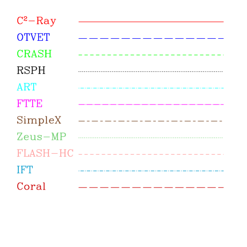
Figure 1: Legend for the line plots.

3 Tests and Results

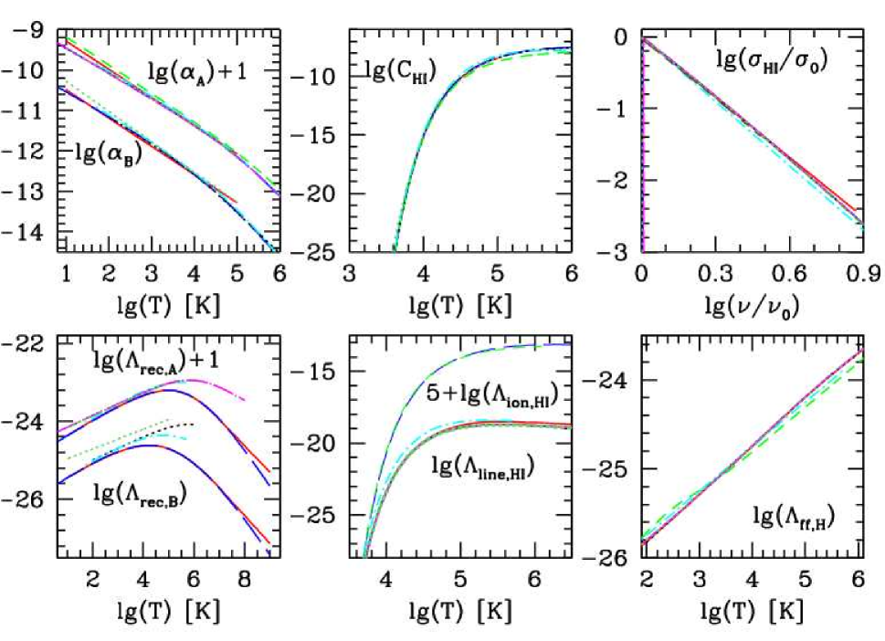
Figure 2: Test 0, part 1: Hydrogen rates, cooling and cross-sections used by the participating codes.

In this section we describe the tests we have performed, along with their detailed parameters, geometry and setup, and the results we obtained. When constructing these tests, we aimed for the simplest and cleanest, but nonetheless cosmologically-interesting problems. We designed them in a way which allows us to test and compare all the important aspects of any radiative-transfer code. These include correct tracking of both slow and fast I-fronts, in homogeneous and inhomogeneous density fields, formation of shadows, spectrum hardening, and solving for the gas temperature state. In a companion paper (Paper II) we will present the tests which include the interaction with fluid flows and radiative feedback on the gas. For simplicity, in all tests the gas is assumed to be hydrogen-only. The gas density distribution is fixed. Finally, in order to be included in the comparison, each test had to be done by at least three or more of the participating codes.

Figure 1 provides a legend allowing the reader to identify which line corresponds to which code in the figures throughout the paper. The images we present are identified in the corresponding figure caption.

All test problems are solved in three dimensions (3D), with grid dimensions $128^{3}$ cells. For the 1D (Zeus-MP) and 2D (Coral) codes the data is interpolated on the same-size 3D grid and analyzed the same way. Unless otherwise noted, the sources of ionizing radiation are assumed to have a black-body spectrum with effective temperature $T_{\rm eff}=100,000$ K, except for Test 1 where the assumed spectrum is monochromatic with all photons having energy $h\nu=13.6$ eV, the ionization threshold of hydrogen. In all tests the temperature is allowed to vary due to atomic heating and cooling processes in accordance with the energy equation, again with the exception of Test 1 where we fix the temperature at $T=10^{4}$ K. The few codes that do not yet include an energy equation use a constant temperature value.

3.1 Test 0: The basic physics

Table 2: Rates adopted by the different radiative transfer codes. The columns are, from left to right, name of the code and reference for: case A recombination rate (RRA) of H II, He II and He III; case B recombination rate (RRB) of H II, He II and He III; dielectronic recombination rate (DRR) of He II; collisional ionization rate (CIR) of H I, He I and He III; collisional ionization cooling rate (CICR) of H I, He I and He II; case A recombination cooling rate (RCRA) of H II, He II and He III; case B recombination cooling rate (RCRB) of H II, He II and He III; dielectronic recombination cooling rate (DRCR) of He II; collisional excitation cooling rate (CECR) of H I, He I and He II; Bremsstrahlung cooling rate (BCR); Compton cooling rate (CCR); cross-section (CS) of H I, He I and He II. Units of RRA, RRB, DRR and CIR are [cm³s^-1], units of CICR, RCRA, RCRB, DRCR, CECR, BCR, CCR are [erg cm³s^-1] and units of CS are [cm²]. Note that for those codes in which the treatment of He is not included, only the references to the H rates are given.

CODE	RRA	RRB	DRR	CIR	CICR	RCRA	RCRB	DRCR	CECR	BCR	CCR	CS
C2-Ray		10,11,10		6			10,11,10		23,-,-	10	18	15
OTVET	9,4,9	9,4,9	2	9,9,9	9,9,9	9,4,9	9,4,9	2	5,-,5		17	22
CRASH	5,5,5	20,20,20	5	5,5,5	5,5,5	5,5,5	20,20,20	5	5,5,5	5	8	15
RSPH		20		18			20		7			18
ART	19	20		19		19	20		19	19	19	13
FTTE	1	9,9,9	1	1,1,1	18,18,18	5,5,5	10,11,10	5	3,5,5	3	16	15
SimpleX		20		6								15
ZEUS-MP	1	21		12	18	5			5,-,-	3	16	14
FLASH-HC		10,11,10		6			10,11,10		23,-,-	10		15
IFT		9		25	5		18		5,-,-	3		22
Coral	10,11,10	10,11,10	24	6	23,23,23	10,11,10	10,11,10	24	23,23,23	10	18	15

(1) Abel et al. (1997); (2) Aldrovandi & Pequignot (1973); (3) Black (1981); (4) Burgess & Seaton (1960); (5) Cen (1992); (6) Cox (1970); (7) Fukugita & Kawasaki (1994); (8) Haiman et al. (1996); (9) Hui & Gnedin (1997); (10) Hummer (1994); (11) Hummer & Storey (1998); (12) Janev et al. (1987); (13) Lang (1974); (14) Osterbrock (1974); (15) Osterbrock (1989); (16) Peebles (1971); (17) Peebles (1993); (18) Shapiro & Kang (1987); (19) Sherman (1979); (20) Spitzer (1978); (21) Tenorio-Tagle et al. (1986); (22) Verner et al. (1996); (23) Aggarwal (1983); (24) Raga et al. (1997); (25) Voronov (1997);
Notes: the codes $C^{2}$-Ray, Flash-HC and Coral all share the same nonequilibrium chemistry module (DORIC, developed by G. Mellema), so they have the same hydrogen chemistry and heating rates and cross-section, and the same chemistry solver. However, Coral also includes the chemistry of helium and a number of metals.

The solution of the radiative transfer equation is intimately related to the ionization and thermal states of the gas. These depend on the atomic physics reaction rates, photoionization cross-sections, as well as cooling and heating rates used. As there is a variety of rates available in the literature, for the sake of clarity we have summarized those used in our codes in Table 2 and plotted them in Figure 2. The table columns indicate, from left to right, the name of the code and the reference for: case A recombination rate of H II, He II and He III; case B recombination rate of H II, He II and He III; dielectronic recombination rate of He II; collisional ionization rate of H I, He I and He III; collisional ionization cooling rate of H I, He I and He II; case A recombination cooling rate of H II, He II and He III; case B recombination cooling rate of H II, He II and He III; dielectronic recombination cooling rate of He II; collisional excitation cooling rate of H I, He I and He II; Bremsstrahlung cooling rate; Compton cooling rate; cross-section of H I, He I and He II. Note that for those codes in which the treatment of He is not included, only the references to the H rates are given.

The first thing to note in Figure 2 is that although the rates come from a wide variety of sources, they largely agree. The main differences are in our recombination cooling rates, particularly at very high temperatures, beyond the typical range of gas temperatures achieved by photoionization heating ($T\mathrel{\hbox{\hbox to0.0pt{\hbox{\lower 4.0pt\hbox{$\sim$}}\hss}\hbox{$<$}}}10^{5}$ K). It should be noted, however, that e.g. shock-heated gas can reach much higher temperatures, in which case the differences in our rates become very large and caution should be excersised in choosing the appropriate rates. However, even at the typical photoionization temperatures there are differences between the rates by up to factors of $\sim 2$. The origin of these discrepancies is currently unclear, and it is also unclear which fit to the experimental data is more precise. There are also a few cases in which particular cooling rates (e.g. Zeus Case B recombination cooling, ART line cooling) are notably different from the rest.

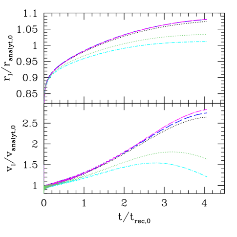
Figure 3: Test 0, part 2: I-front expansion in uniform-density field with temperature evolution (same as Test 2 below). Plotted are the I-front position (top) and velocity (bottom) all derived from the same code (1D, spherically-symmetric version of ART code) and using the photoionization cross-section from that code, but with the rest of the microphysics (chemistry and cooling rates) taken from several of the participating codes, as indicated by line-type and color. All results are normalized to the analytical ones (which assume fixed temperature, $T=10^{4}$ K) given in equations (6) below (see text for details).

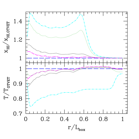
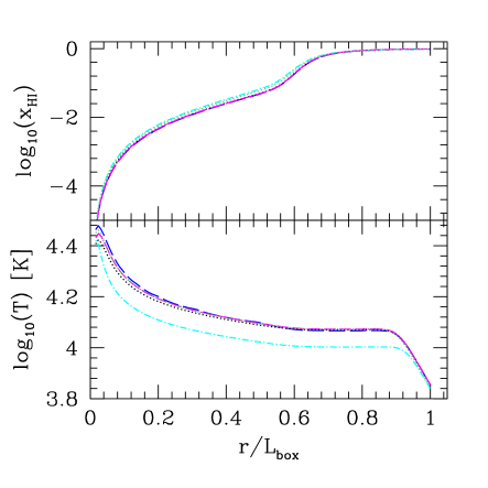
Figure 4: Test 0, part 2: Same test as in Fig. 3. (left) (a) The radial profiles of the neutral fraction (top, normalized to the result which uses the OTVET rates), temperature (middle, again normalized to the results for OTVET rates) at time $t=100$ Myr$=0.82t_{\rm rec,0}$. (right) (b) The same as in (a) but in absolute units.

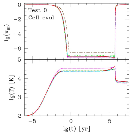
Figure 5: Test 0, part 3: Single-zone ionizing up and cooling and recombining.

As a next step, we did several numerical experiments to assess the offsets between our results that can arise solely based on our different chemistry and cooling rates. We did this by implementing the rates from several codes representative of the full range of rates present above into a single code (1-D version of ART code) and running the same problem (Test 2 described below, which is expansion of an H II region in uniform density gas, see § 3.3 for detailed test definition and solution features). In all cases the same photoionization cross-section (the one of ART) is used and only the rates are varied. The code OTVET here stands also for the codes $C^{2}$-Ray, CRASH, Flash-HC and Coral, since all these codes have either identical, or closely-matching rates. Results are shown in Figures 3 and 4. In Figure 3 we show the I-front position, $r_{I}$, and the I-front velocity, $v_{I}$ (Both quantities are normalized to the analytical solutions of that problem obtained at temperature $T=10^{4}$ K, while the time is in units of the recombination time at the same temperature). Note that the results for Zeus use the recombination cooling rate of ART since its currently-implemented rate is overly-simplified. We show the results using the rates of OTVET, FTTE, RSPH, Zeus-MP and ART.

Initially, when the I-front is fast and still far away from reaching its Strömgren sphere the results for all codes agree fairly well, as expected since recombinations are still unimportant. Once recombinations do become important, at $t>t_{\rm rec}$, the results start diverging. The results for OTVET, FTTE and RSPH remain in close agreement, within a fraction of once per cent in the I-front radius and within $\sim 2\%$ in the I-front velocity. The results using the Zeus and ART rates however depart noticeably from the others, by up to 4% and 6, respectively in radius. The corresponding velocities are different even more, by up to factor of $\sim 2$ at the end, when the I-front is close to stationary. In Figure 4 we show the radial profiles of the ionized fraction $x$, and temperature $T$, normalized to the results using OTVET rates (left), and in absolute units (right). The ionized fraction profiles for ART and Zeus again are fairly different from the rest, by 20-40%, while the rest of the codes agree between themselves much better, to less than 10%. Agreement is slightly worse close to the ionizing source. In terms of temperature profiles the codes agree to better than 10%, with the exception of ART, in which case the resulting temperature is noticeably lower, by $\sim 20\%$.

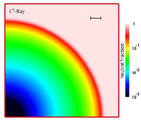
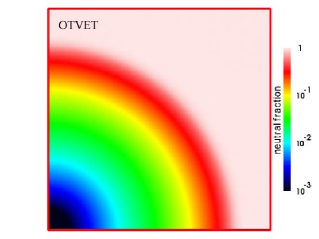
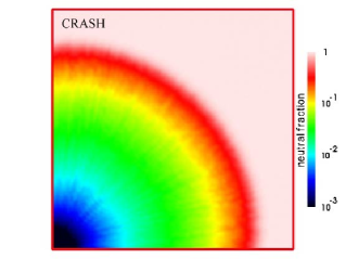
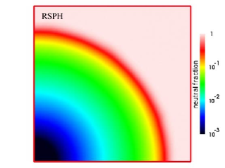
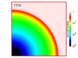
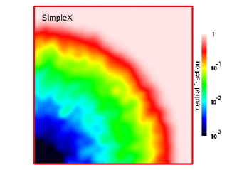
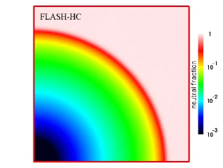
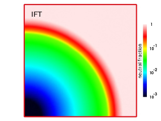
Figure 6: Test 1 (H II region expansion in an uniform gas at fixed temperature): Images of the H I fraction, cut through the simulation volume at coordinate $z=0$ at time $t=500$ Myr (final Strömgren sphere) for (left to right and top to bottom) $C^{2}$-Ray, OTVET, CRASH, RSPH, ART, FTTE, SimpleX, FLASH-HC, and IFT.

The reasons for these discrepancies lie largely in differences in the recombination rates and the recombination and line cooling rates. The line cooling rate of ART is larger than the ones for most of the other codes by a factor of 2 - 5 in the temperature range $10^{4}-10^{5}$ K, while the recombination rate used by that code is about 10-15 percent larger in the same temperature range, thus the resulting gas temperature is correspondingly lower. This lower temperature results in a higher recombination rate and hence the slower propagation of the I-front we observed. The reason for the discrepancy with Zeus is mostly due to its higher recombination rate. This again results in a somewhat slower I-front propagation, but not in significant temperature differences. Accordingly, for both of these codes the neutral gas fraction is significantly higher at all radii. The slightly higher recombination cooling of RSPH results in slightly lower temperature and proportionally higher neutral fraction, although both are off by only a few percent, and up to 10% close to the ionizing source.

The last important element in this basic physics comparison is to assess the accuracy and robustness of the methods we use for solving the non-equilibrium chemistry equations. These equations are stiff and thus generally require implicit solution methods. Such methods are generally expensive, however, so often certain approximations are used to speed-up the calculations. In order to test them, we performed the following simple test with a single, optically thin zone. We start with a completely neutral zone at time $t=0$. We then applied photoionizing flux of $F=10^{12}\,\rm photons/s/cm^{2}$, with $10^{5}$ K black-body spectrum for 0.5 Myr, which results in the gas parcel becoming heated and highly ionized. Thereafter, the ionizing flux is switched off and the zone cools down and recombines for further 5 Myr. The zone contains only hydrogen gas with number density of $n=1\,cm^{-3}$, and initial temperature of $T_{i}=100$ K. Our results are shown in Figure 5.

All codes agree very well in terms of the evolution of the neutral fraction (top panel), with the sole exception of SimpleX, in which case both the speed with which the gas parcel ionizes up and the achieved level of ionization are significantly different from the rest. The reason for this discrepancy is that currently this code does not solve the energy equation to find the gas temperature but has to assume a value instead ($T=10^{4}$ K in this test). FTTE finds slightly higher temperatures after its initial rise and correspondingly lower neutral fractions.

Some differences are also seen after time $t\sim 0.1$ Myr, at which point there is a slight rise in temperature and corresponding dip in the neutral fraction. These occur around the time when the recombinations start becoming important, since $t_{\rm rec}\sim 0.1$ Myr, which gives rise to slight additional heating. About half of the codes predict somewhat lower temperature rise then the rest. The cooling/recombination phase after source turn off demonstrates good agreement between the codes, although there is small difference in the final temperatures reached which is due to small differences in the hydrogen line cooling rates, resulting in slightly different temperatures at which the cooling becomes inefficient.

3.2 Test 1: Pure-hydrogen isothermal H II region expansion

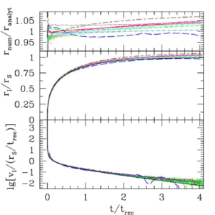
Figure 7: Test 1 (H II region expansion in an uniform gas at fixed temperature): The evolution of the position and velocity of the I-front.

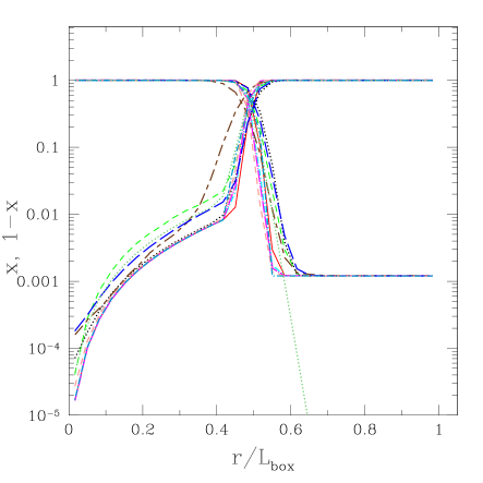
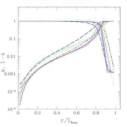
Figure 8: Test 1 (H II region expansion in an uniform gas at fixed temperature): Spherically-averaged profiles for ionized fractions $x$ and neutral fractions $x_{\rm HI}=1-x$ at times $t=30$ Myr and 500 Myr vs. dimensionless radius (in units of the box size).

This test is the classical problem of an H II region expansion in an uniform gas around a single ionizing source (Strömgren 1939; Spitzer 1978). A steady, monochromatic ($h\nu=13.6$ eV) source emitting $\dot{N}_{\gamma}$ ionizing photons per unit time is turning on in an initially-neutral, uniform-density, static environment with hydrogen number density $n_{H}$. For this test we assume that the temperature is fixed at $T=10^{4}$ K. Under these conditions, and if we assume that the front is sharp (i.e. that it is infinitely-thin, with the gas inside fully-ionized and the gas outside fully-neutral) there is a well-known analytical solution for the evolution of the I-front radius, $r_{I}$, and velocity, $\rm v_{I}$, given by

$$r_{I} = r_{\rm S}\left[1-\exp(-t/t_{\rm rec})\right]^{1/3}\,,$$ (5)

$$\rm v_{I} = \frac{r_{\rm S}}{3t_{\rm rec}}\frac{\exp{(-t/t_{\rm rec})}}{\left[1-\exp(-t/t_{\rm rec})\right]^{2/3}}\,,$$ (6)

where

$$r_{\rm S}=\left[{3\dot{N}_{\gamma}\over 4\pi\alpha_{B}(T)n_{\rm H}^{2}}\right]^{1/3}\,,$$ (7)

is the Strömgren radius, i.e. the final, maximum size of the ionized region at which point recombinations inside it balance the incoming photons and the H II region expansion stops. The Strömgren radius is obtained from

$$F=\int_{0}^{r_{S}}d\ell n_{e}n_{H}\alpha_{B}(T),$$ (8)

i.e. by balancing the number of recombinations with the number of ionizing photons arriving along a given line of sight (LOS). Here $n_{e}$ is the electron density,

$$t_{\rm rec}=\left[\alpha_{B}(T)n_{\rm H}\right]^{-1}\,,$$ (9)

is the recombination time, and $\alpha_{B}(T)$ is the Case B recombination coefficient of hydrogen in the ionized region at temperature $T$. The H II region initially expands quickly and then slows considerably as the evolution time approaches the recombination time, $t\sim t_{\rm rec}$, at which point the recombinations start balancing the ionizations and the H II region approaches its Strömgren radius. At a few recombination times I-front stops at radius $r_{I}=r_{S}$ and in absence of gas motions remains static thereafter. The photon mean-free-path is given by

$$\lambda_{\rm mfp}=\frac{1}{n_{H}\sigma_{0}}=0.041\,\rm pc.$$ (10)

The particular numerical parameters we used for this test are as follows: computational box dimension $L=6.6$ kpc, gas number density $n_{H}=10^{-3}$ cm^-3, initial ionization fraction (given by collisional equilibrium) $x=1.2\times 10^{-3}$, and ionization rate $\dot{N}_{\gamma}=5\times 10^{48}$ photons s^-1. The source is at the corner of the box). For these parameters the recombination time is $t_{\rm rec}=3.86\times 10^{15}\,\rm s=122.4$ Myr. Assuming a recombination rate $\alpha_{B}(T)=2.59\times 10^{-13}\rm\,cm^{3}s^{-1}$ at $T=10^{4}$ K, then $r_{S}=5.4$ kpc. The simulation time is $t_{\rm sim}=500$ Myr $\approx 4\,t_{\rm rec}$. The required outputs are the neutral fraction of hydrogen on the whole grid at times $t=10,30,100,200,$ and 500 Myr, and the I-front position (defined by the 50% neutral fraction) and velocity vs. time along the $x$-axis.

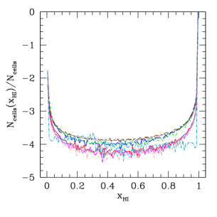
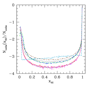
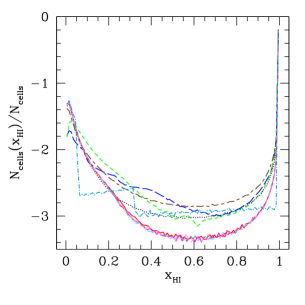
Figure 9: Test 1 (H II region expansion in an uniform gas at fixed temperature): Fraction of cells with a given neutral fraction, $x_{\rm HI}=1-x$ at times (left) $t=10$ Myr, (middle) 100 Myr and (right) 500 Myr.

In Figure 6 we show images of the neutral fraction in the $z=0$ plane at time $t=500$ Myr, at which point the equilibrium Strömgren sphere is reached. The size of the final ionized region is in very good agreement between the codes. In most cases the H II region is nicely spherical, although some anisotropies exist in the CRASH and SimpleX results. In the first case these are due to the Monte-Carlo random sampling nature of this code, while in the second case it is due to the unstructured grid used by that code, which had to be interpolated on the regular grid format used for this comparison. There are also certain differences in the H II region ionized structure, e.g. in the thickness of the ionized-neutral transition at the Strömgren sphere boundary. The inherent thickness of this transition (defined as the radial distance between 0.1 and 0.9 ionized fraction points) for monochromatic spectrum is $\approx 18\lambda_{\rm mfp}=0.74$ kpc, or about 14 simulation cells, equal to 11% of the simulation box size. This thickness is indicated in the upper left panel of Figure 6. Most codes find widths which are very close to this expected value. Only the OTVET, CRASH and SimpleX codes find thicker transitions due to the inherently greater diffusivity of these methods, which spreads out the transition. For the same reason the highly-ionized proximity region of the source (blue-black colors) is noticeably smaller for the same two codes.

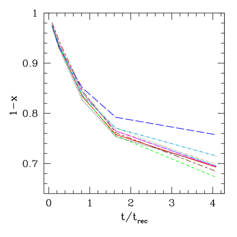
Figure 10: Test 1 (H II region expansion in an uniform gas at fixed temperature): Evolution of the total neutral fraction.

In Figure 7 we show the evolution of the I-front position and velocity. The analytical results in equation (6) are shown as well (black, solid lines). All codes track the I-front correctly, with the position never varying by more than 5% from the analytical solution. These small differences are partly due to differences in our recombination rates, as discussed above, and partly a consequence of our (somewhat arbitrary) definition of the I-front position as the point of 50% ionization. Our chosen parameters are such that the I-front internal structure is well-resolved, and the I-front intrinsic thickness is larger than the discrepancies between the different codes. The IFT code in particular tracks the I-front almost perfectly, as is expected for this code by construction. The ray-tracing codes agree between themselves a bit better than they do with the moment-based method OTVET. This is again related to the different, somewhat more diffusive nature of the last code. The I-front velocities also show excellent agreement with the analytical result, at least until late times (at few recombination times), at which point the I-front essentially stops and its remaining slow motion forward is not possible to resolve with the relatively coarse resolution adopted for our test. The I-front at this point is moving so slowly that most of its remaining motion takes place within a single grid cell for extended periods of time and thus falls below our resolution there.

In Figure 8 we plot the spherically-averaged radial profiles of the ionized and the neutral fraction. In the left panel we show these profiles at $t=30$ Myr, during the early, fast expansion of the I-front. Most of the ray-tracing codes ($C^{2}$-Ray, ART, FLASH-HC and IFT) agree excellently at all radii. The OTVET, CRASH and SimpleX codes appear more diffusive, finding a thicker I-front transition and lower ionized fraction inside the H II region. The Zeus code also derives lower ionized fractions inside the H II region due to its slightly higher recombinational coefficient. The RSPH code is intermediate between the two groups of codes, finding essentially the same neutral gas profile inside the H II region as the ray-tracing codes, but a slightly thicker I-front, i.e. the ionized fraction drops more slowly ahead of the I-front.

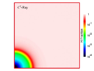
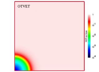
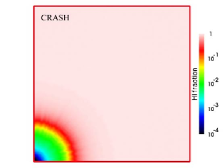
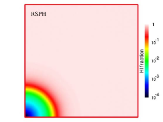
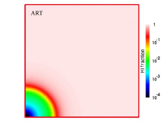
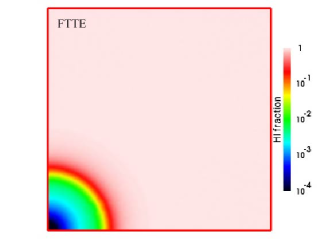
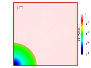
Figure 11: Test 2 (H II region expansion in an uniform gas with varying temperature): Images of the H I fraction, cut through the simulation volume at coordinate $z=0$ at time $t=10$ Myr for (left to right and top to bottom) $C^{2}$-Ray, OTVET, CRASH, RSPH, ART, FTTE, and IFT.

The same differences persist in the ionized structure of the final Strömgren sphere at $t=500$ Myr (Figure 8, left panel). The majority of the ray-tracing codes again agree fairly well. The IFT code is based on the exact analytical solution of this particular problem, and thus to a significant extent could be considered a substitute for the analytical H II region structure. Its differences from the exact solution are only close to the I-front, where the non-equilibrium effects dominate, while IFT currently assumes equilibrium chemistry. Away from the I-front, however, the ionized state of the gas is in equilibrium and there all ray-tracing codes agree perfectly. The SimpleX, OTVET and CRASH codes find thicker sphere boundaries and lower ionized fractions inside, but the first two codes find slightly smaller Strömgren spheres, while the last finds a slightly larger one. The Zeus code finds lower ionized fractions inside the ionized region and a somewhat thicker I-front, but an overall H II region size that agrees with the other ray-tracing codes. The lower ionization is due to the current restriction of Zeus to monochromatic radiative transfer, with its lower postfront temperatures and hence higher recombination rates.

In Figure 9 we show histograms of the fraction of cells with a given neutral fraction during the early, fast expansion phase (at time $t=10$ Myr; left), when it starts slowing down ($t=100$ Myr, close to one recombination time; middle), and when the final Strömgren sphere is reached ($t=500$ Myr; right). These histograms reflect the differences in the I-front transition thickness and internal structure. All codes predict a transitional region of similar size, which contains a few percent of the total volume. In detail, however, once again the results fall into two main groups. One group includes most of the ray-tracing codes, which agree perfectly at all times and predict thin I-fronts close to the analytical prediction. The other group includes the more diffusive schemes, namely OTVET, CRASH, RSPH and SimpleX, which all find somewhat thicker I-fronts. During the expansion phase of the H II region these three codes agree well between themselves, but they disagree somewhat on the structure of the final equilibrium Strömgren sphere, particularly in the proximity region of the source. The IFT code histograms differ significantly from the rest, due to its assumed equilibrium chemistry, which is not quite correct at the I-front.

Finally, the evolution of the globally-averaged neutral fractions is shown in Figure 10. The same trends are evident, with the ray-tracing codes agreeing closely among themselves, while the OTVET finds about 10% more neutral material at the final time, due to the different ionization structure obtained by this method.

3.3 Test 2: H II region expansion: the temperature state

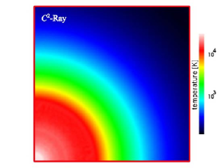
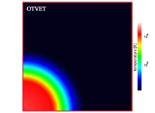
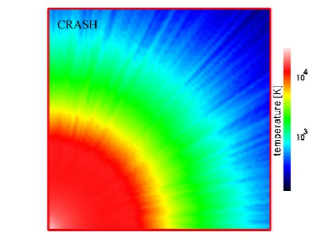
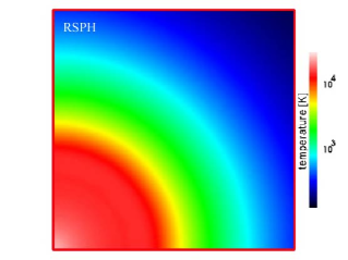
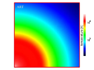
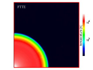
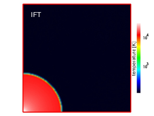
Figure 12: Test 2 (H II region expansion in an uniform gas with varying temperature): Images of the temperature, cut through the simulation volume at coordinate $z=0$ at time $t=10$ Myr for (left to right and top to bottom) $C^{2}$-Ray, OTVET, CRASH, RSPH, ART, FTTE, and IFT.

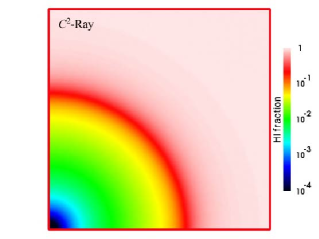
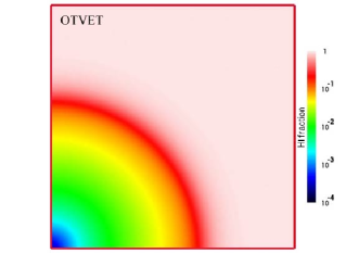
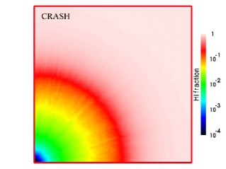
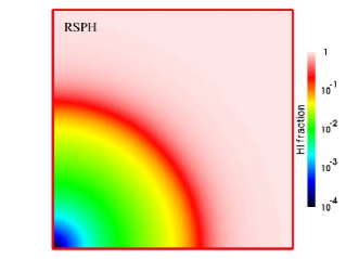
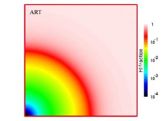
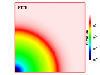
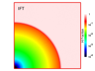
Figure 13: Test 2 (H II region expansion in an uniform gas with varying temperature): Images of the H I fraction, cut through the simulation volume at coordinate $z=0$ at time $t=100$ Myr for (left to right and top to bottom) $C^{2}$-Ray, OTVET, CRASH, RSPH, ART, FTTE, and IFT.

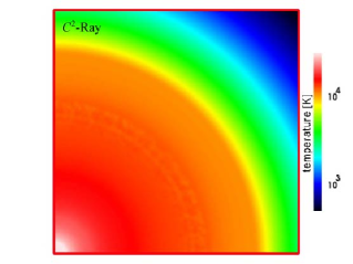
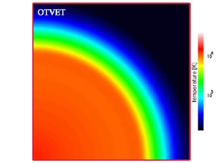
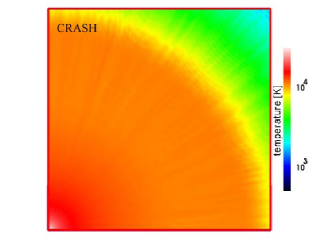
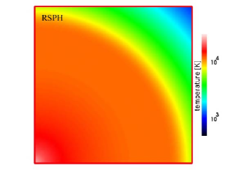
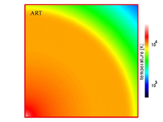
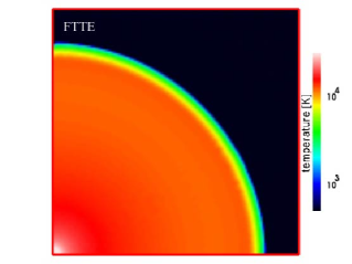
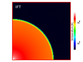
Figure 14: Test 2 (H II region expansion in an uniform gas with varying temperature): Images of the temperature, cut through the simulation volume at coordinate $z=0$ at time $t=100$ Myr for (left to right and top to bottom) $C^{2}$-Ray, OTVET, CRASH, RSPH, ART, FTTE, and IFT.

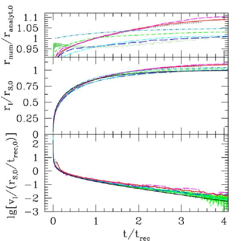
Figure 15: Test 2 (H II region expansion in an uniform gas with varying temperature): The evolution of the position and velocity of the I-front.

Test 2 solves essentially the same problem as Test 1, but the ionizing source is assumed to have a $10^{5}$ K black-body spectrum and we allow the gas temperature to vary due to heating and cooling processes, as determined by the energy equation. The test geometry and gas density are the same as in Test 1. The gas is initially fully neutral and has a temperature of $T=100$ K.

In Figure 11 we show images of the neutral fraction on the $z=0$ plane at time $t=10$ Myr, during the initial fast expansion phase of the H II region. All of the results agree fairly well on the overall size of the ionized region and its internal structure. Again there are modest differences in the thickness of the I-front and the ionizing source proximity region, e.g. the CRASH code again produces a somewhat thicker transition and smaller proximity region. The IFT code finds significantly sharper I-fronts due to its equilibrium chemistry, but the internal H II region structure away from the front (which is close to equilibrium) and overall size of the ionized region both agree well with the rest of the codes. The temperature structure of the H II region, on the other hand, demonstrates significant differences (Figure 12). These stem largely from the different way the codes handle spectrum hardening, i.e. the long mean free paths of the high-energy photons due to the much lower photoionization cross-section at high frequencies. These long mean free paths result in a much thicker I-front transition and a significant pre-heating ahead of the actual I-front, since the high energy photons heat the gas, but there are not enough of them to ionize it. The CRASH code, which follows multiple bins in frequency, finds a larger pre-heated region than the other codes. There are also significant anisotropies in the CRASH results, due to the Monte-Carlo sampling method used (since not many high-energy photon packets are sent, leading to undersampling in angle). In production runs, a multifrequency treatment of the single photon packets has been introduced, reducing the anisotropies in the results. The temperature results of $C^{2}$-Ray, RSPH and ART codes agree fairly well among themselves, while OTVET and FTTE give much less spectrum hardening. Finally, IFT assumes the I-front is sharp, and does not have spectrum hardening by construction.

The same trends persist at later times, when the I-front is approaching the Strömgren sphere (Figures 13 and 14). Once again the H II regions predicted by all the codes are similar in size and internal structure, but with a little different I-front thickness in terms of neutral fraction and significant differences in terms of spectral hardening. The FTTE still gives a very sharp I-front, while OTVET finds somewhat less hardening, but its later-time result is more similar to the other codes than at early times.

In Figure 15 we plot the the position and velocity of the I-front vs. time. Unlike Test 1, in this case there is no closed-form analytical solution since the recombination coefficients vary with the spatially-varying temperature. Nevertheless, as a point of reference we have again shown the analytical solution in equations (6) (assuming $T=10^{4}$ K). All the codes find slightly larger H II regions and slightly faster I-front propagation compared to this analytical solution. This is to be expected due to the temperature being higher than $10^{4}$ K and the inverse temperature dependence of the recombination coefficient. The $C^{2}$-Ray, RSPH and FTTE results agree perfectly among themselves, to $\sim 1\%$, as do the results from OTVET, ART, and Zeus, again among themselves. These two groups of results differ by $\sim 10\%$, however, while CRASH and IFT find an H II region size intermediate between the two groups.

In Figure 16 we show the spherically-averaged radial profiles of the neutral and ionized fractions during the fast expansion phase ($t=10$ Myr, left), the slowing-down phase ($t=100$ Myr, middle) and the final Strömgren sphere ($t=500$ Myr, right). These confirm, in a more quantitative way, the trends already noted based on the 2D images above. The profiles from $C^{2}$-Ray and RSPH codes are in excellent agreement at all radii and all times. The IFT code closely agrees with them in the source proximity region, where the gas ionized state is at equilibrium, but diverges around the I-front (due to its assumed equilibrium chemistry) and ahead of the I-front (due to its assumption that the front is sharp). Compared to these codes, CRASH and ART find slightly higher neutral fractions close to the ionizing source, but agree well with $C^{2}$-Ray and RSPH ahead of the I-front in the spectral hardening region. The FTTE code is in excellent agreement with $C^{2}$-Ray and RSPH codes close to the source, but its I-front is much sharper. The OTVET code also finds a somewhat sharper I-front, but to a much lesser extent than the FTTE code, while close to the source its neutral fraction is only slightly higher than the majority of codes, and in close agreement with the ART code. Finally, the I-front derived by the Zeus code is very sharp. This is due to the use of only single-energy photons by this code, which does not allow for spectral hardening.

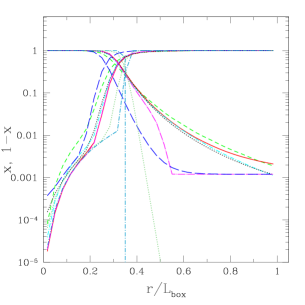
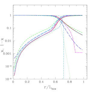
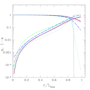
Figure 16: Test 2 (H II region expansion in an uniform gas with varying temperature): Spherically-averaged ionized fraction $x$ and neutral fraction $1-x$ profiles at times $t=10$ Myr, 100 Myr and 500 Myr.

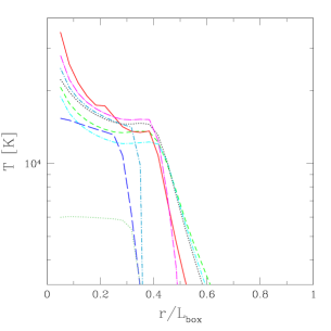
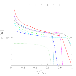
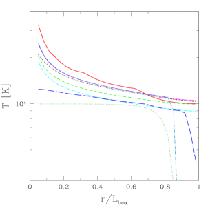
Figure 17: Test 2 (H II region expansion in an uniform gas with varying temperature): Spherically-averaged temperature profiles at times $t=10$ Myr, 100 Myr and 500 Myr.

The corresponding spherically-averaged radial temperature profiles at the same three I-front evolutionary phases are shown in Figure 17. All results (except the one from Zeus, due to the monochromatic spectrum it used) agree well inside the ionized region, with the differences arising largely due to slight differences in the cooling rates adopted. The more diffusive OTVET code does not show as sharp temperature rise in the source proximity as the other codes, but elsewhere the temperature structure it finds agrees with the majority of the codes. Again at the I-front and ahead of it the differences between the results are significant, reflecting the different handling of hard photons by the codes.

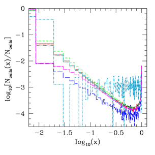
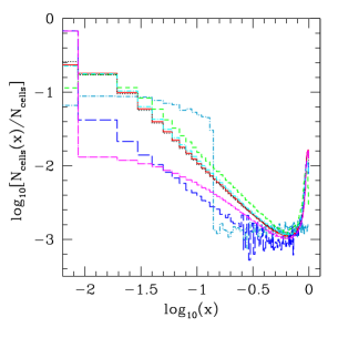
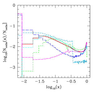
Figure 18: Test 2 (H II region expansion in an uniform gas with varying temperature): Fraction of cells with a given ionized fraction, $x$, at times (left) $t=10$ Myr, (middle) 100 Myr and (right) 500 Myr.

In Figure 18 we show the histograms of the fraction of cells with a given ionized fraction $x$ at the same times as the radial profiles above. During the early, fast expansion phase all codes agree well except the OTVET code, which finds a slightly thinner I-front, but an otherwise same histogram distribution shape, and CRASH, whose I-front is a bit thicker. IFT finds a different ionized fraction distribution, again as a consequence of its equilibrium chemistry, which is not correct at the I-front transition. Later, when the I-front slows down ($t=100$ Myr) the same trends hold, but in addition the FTTE results start diverging significantly from the rest, finding notably smaller ionized region and a quite different shape distribution in the largely-neutral regions. This reflects its much sharper I-front with little spectrum hardening, as noted above. Finally, the ionized fraction histogram corresponding to the Strömgren sphere ($T=500$ Myr) shows similar differences. The $C^{2}$-Ray, ART and RSPH codes again agree very closely, and CRASH also finds a similar distribution, but with a thicker I-front and correspondingly fewer neutral cells. The OTVET distribution follows a roughly similar shape but with a thinner front transition and more neutral cells, while FTTE agrees well with the other ray-tracing codes in the highly-ionized region, but still diverges considerably at the I-front and ahead of it.

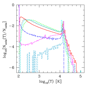
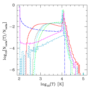
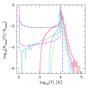
Figure 19: Test 2 (H II region expansion in an uniform gas with varying temperature): Fraction of cells with a given temperature $T$ at times (left) $t=10$ Myr, (middle) 100 Myr and (right) 500 Myr.

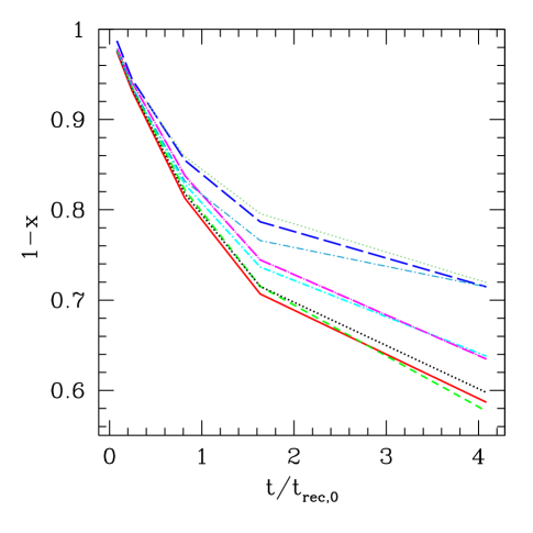
Figure 20: Test 2 (H II region expansion in an uniform gas with varying temperature): Evolution of the total neutral gas fraction.

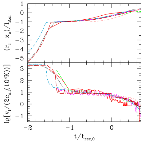
Figure 21: Test 3 (I-front trapping in dense clump): The evolution of the position and velocity of the I-front.

The corresponding histograms of temperature are shown in Figure 19. The ionized gas temperatures found by all codes have a strong peak at slightly above $10^{4}$ K, with only small variations in the peak position between the different codes. This peak was to be expected, as a consequence of the combination of photoheating and hydrogen line cooling (which peaks around $10^{4}$ K). At higher temperatures (corresponding to cells close to the ionizing source) some differences emerge. The ray-tracing codes ($C^{2}$-Ray, CRASH, ART, RSPH, IFFT, IFT) largely agree among themselves, with only $C^{2}$-ray finding slightly larger fraction of hot cells. OTVET, on the other hand does not predict any cells with temperature above $\sim 16,000$ K, due to missing the very hot proximity region of the source, as noted above. Below $\sim 8,000$ K, on the other hand, the differences between results are more significant, reflecting the variations in the I-front thickness and spectral hardening noted above. The results from CRASH, ART and RSPH agree well at all times, while the $C^{2}$-Ray histograms have similar shape, but with some offset, due to its current somewhat simplified handling of the energy input which uses a single bin in frequency. The OTVET, FTTE and IFT codes find much smaller pre-heating ahead of the I-front, and thus different distributions.

Finally, in Figure 20 we show the evolution of the total neutral gas fraction. All codes agree well on the final neutral fraction, within $\sim 25\%$ or better. The differences are readily understood in terms of the different recombination rates, mostly as a consequence of the somewhat different temperatures found inside the H II region, in addition to the small differences in the recombination rate fits used.

3.4 Test 3: I-front trapping in a dense clump and the formation of a shadow.

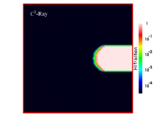
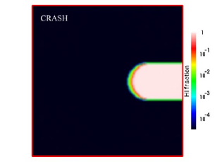
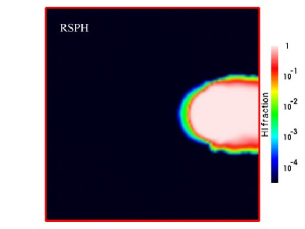
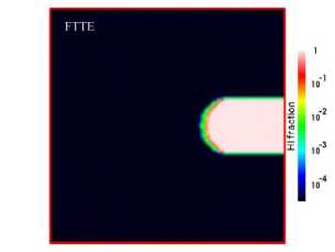
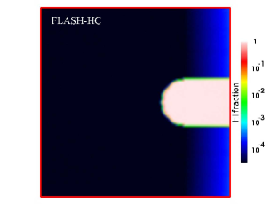
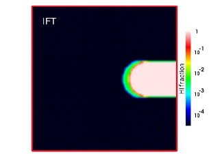
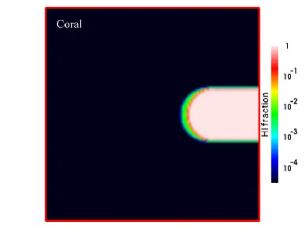
Figure 22: Test 3 (I-front trapping in dense clump): Images of the H I fraction, cut through the simulation volume at midplane at time $t=1$ Myr for $C^{2}$-Ray, CRASH, RSPH, FTTE, Flash-HC, IFT and Coral.

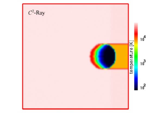
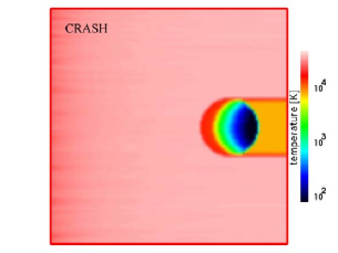
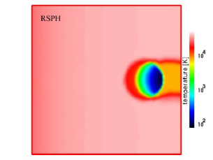
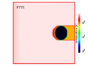
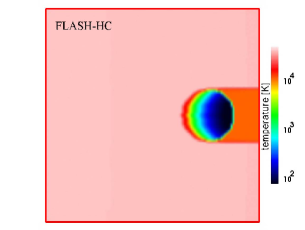
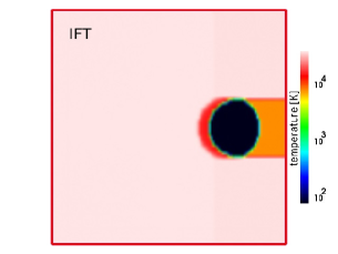
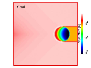
Figure 23: Test 3 (I-front trapping in dense clump): Images of the temperature, cut through the simulation volume at midplane at time $t=1$ Myr for $C^{2}$-Ray, CRASH, RSPH, FTTE, Flash-HC, IFT and Coral.

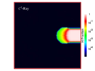
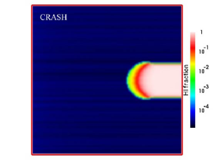
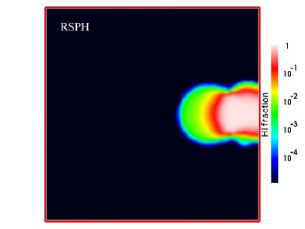
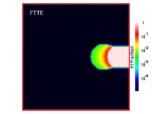
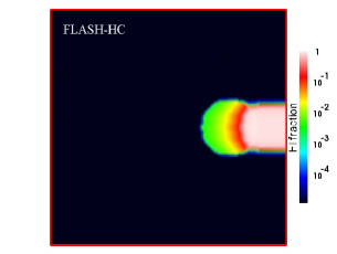
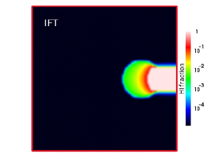
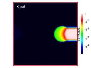
Figure 24: Test 3 (I-front trapping in dense clump): Images of the H I fraction, cut through the simulation volume at midplane at time $t=15$ Myr for $C^{2}$-Ray, CRASH, RSPH, FTTE, Flash-HC, IFT and Coral.

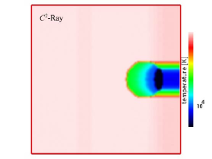
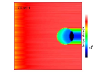
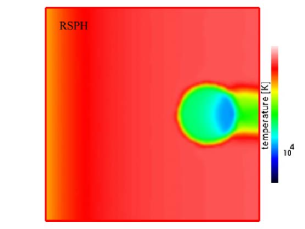
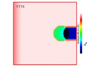
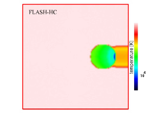
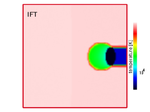
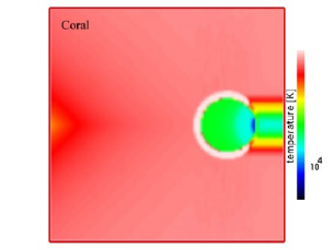
Figure 25: Test 3 (I-front trapping in dense clump): Images of the temperature, cut through the simulation volume at midplane at time $t=15$ Myr for $C^{2}$-Ray, CRASH, RSPH, FTTE, Flash-HC, IFT and Coral.

Test 3 examines the propagation of a plane-parallel I-front and its trapping by a dense, uniform, spherical clump. The condition for an I-front to be trapped by a clump of gas with number density $n_{H}$ can be derived as follows (Shapiro et al. 2004). Let us define the Strömgren length $\ell_{S}(r)$ at impact parameter $r$ from the clump center using equation (8), but in this case following lines-of-sight for each impact parameter. We then can define the “Strömgren number” for the clump as $L_{S}\equiv 2r_{\rm clump}/\ell_{S}(0)$, where $r_{\rm clump}$ is the clump radius and $\ell_{S}(0)$ is the Strömgren length at zero impact parameter. Then, if $L_{S}>1$ the clump is able to trap the I-front, while if $L_{S}<1$, the clump would be unable to trap the I-front and instead would be flash-ionized by its passage.

For a uniform-density clump equation (8) reduces to

$$\ell_{S}=\frac{F}{\alpha_{H}^{(2)}n_{H}^{2}},$$ (11)

and the Strömgren number is given by

$$L_{S}=\frac{2r_{\rm clump}\alpha_{B}(T)n_{H}^{2}}{F}.$$ (12)

The numerical parameters for Test 3 are as follows: the spectrum is a black-body with effective temperature $T_{eff}=10^{5}$ K and constant ionizing photon flux, $F=10^{6}\rm\,s^{-1}cm^{-2}$, incident to the $y=0$ box side; the hydrogen number density and initial temperature of the environment are $n_{\rm out}=2\times 10^{-4}\rm\,cm^{-3}$ and $T_{\rm out,init}=8,000$ K, while inside the clump they are $n_{\rm clump}=200n_{\rm out}=0.04\rm\,cm^{-3}$ and $T_{\rm clump,init}=40$ K. The box size is $L=6.6$ kpc, the radius of the clump is $r_{\rm clump}=0.8$ kpc, and its center is at $(x_{c},y_{c},z_{c})=(5,3.3,3.3)$ kpc, or $(x_{c},y_{c},z_{c})=(97,64,64)$ cells, and the evolution time is 15 Myr. For these parameters and assuming for simplicity that the Case B recombination coefficient is given by $\alpha_{B}(T)=2.59\times 10^{-13}(T/10^{4}\,K)^{-3/4}$, we obtain $\ell_{S}\approx 0.78(T/10^{4}\,K)^{3/4}$ kpc, and $L_{S}\approx 2.05(T/10^{4}\,K)^{-3/4}$; thus, along the axis of symmetry the I-front should be trapped approximately at the center of the clump for $T=10^{4}$ K. In reality, the temperature could be expected to be somewhat different and spatially-varying, but to a rough first approximation this estimate should hold.

In fact, the I-front does get trapped as expected, slightly beyond the clump center. In Figure 21 we plot $(r_{I}-x_{c})/\ell_{S}$, the evolution of the position of the I-front with respect to the clump center in units of the Strömgren length (top panel) and the corresponding velocity evolution (in units of $2c_{s,I}(T=10^{4}\rm K)=2(p/\rho)^{1/2}$, twice the isothermal sound speed in gas at temperature of $10^{4}$ K), both vs. $t/t_{\rm rec,0}$, time in units of the recombination time inside the clump (which is $\sim 3$ Myr at $10^{4}$ K). The I-front is initially highly supersonic due to the low density outside the clump. Once it enters the clump it shows down sharply, to about 20 times the sound speed, by the same factor as the density jump at the clump boundary. As it penetrates further into the clump it approaches its (inverse, i.e. outside-in) Strömgren radius at time $t\sim t_{\rm rec,0}$, at which point the propagation slows down even further until the I-front is trapped after a few recombination times. The velocity drops below $2c_{s,I}$, at which point if gas motions were allowed the I-front would become slow D-type (i.e. coupled to the gas motion, rather than much faster than them). All codes capture these basic phases of the trapping process correctly and agree well on both the front position and velocity. We note here that the FLASH-HC code currently does not have the ability to track fast I-fronts, so its data starts only after the front has slowed down. The IFT method assumes a sharp front, and thus does not allow pre-heating and partial ionization ahead of the front, which results in its being slowed down more abruptly than is the case for the other results. Due to some diffusion, the RSPH code finds that the front slows down slightly before the I-front actually enters the clump. There are also minor differences in the later stages of the evolution, to be discussed in more detail below.

In Figure 22 we show the images of the neutral gas fraction on the plane through the centre of the clump at time $t=1$ Myr, when the I-front is already inside the clump, but still not trapped and moving supersonically. The ionizing source is far to the left of the box. All results show a sharp shadow behind the clump, as expected for such a dense, optically-thick clump. Only the RSPH code shows diffusion at the shadow boundaries, due to the intrinsic difficulty of representing such a sharply-discontinuous density distribution with SPH particles and the corresponding smoothing kernel. The FLASH-HC code derives a noticeably sharper I-front in both the clump and the external medium (where it is the only result to still have some gas with neutral fraction above $\sim 10^{-4}$). This is due to its current inability to correctly track fast I-fronts, as discussed above, which leads to somewhat incorrect early evolution. The corresponding temperature image cuts (Figure 23) show the same trends: FLASH-HC and IFT find a very sharp transition, while the rest of the codes agree reasonably well, with only minor differences in the pre-heating region.

In Figure 24 we show the images of the neutral fraction at the final time of the simulation, $t=15$ Myr. All codes except CRASH find very similar ionized structure inside the clump. The CRASH result has significantly higher neutral fraction inside the clump, and correspondingly larger shadow behind the clump, as well as slightly higher neutral gas fraction in the low-density gas. This could be due to the fact that, as mentioned in § 3.3, CRASH follows multiple bins in frequency over a wider frequency range with respect to the other codes; this results in a higher ionizing power at high frequencies, which also have smaller photo-ionization cross-sections. This in turn could be the origin of the lower ionization state of the clump and of the low-density gas. The RSPH result again exhibits significant diffusion around the edges of the shadow. The corresponding temperature structures, on the other hand, (Figure 25) show some differences, which stem from the different treatments of the energy equation and spectral hardening by the codes. The FTTE and IFT codes find almost no pre-heating in the shielded region and the shadow behind it. $C^{2}$-Ray and CRASH get smaller self-shielded regions and some hard photons penetrating into the sides of the shadow. Finally, RSPH, FLASH-HC and Coral find almost no gas that is completely self-shielded, but still find sufficient column densities to create temperature-stratified shadows similar to the ones found by $C^{2}$-Ray and CRASH codes, albeit at higher temperature levels. The Coral result also has a thin, highly-heated shell at the source side of the clump, resulting from this code’s problems in properly finding the temperature state in the first dense, optically-thick cells encountered by its rays, which leads to their overheating. In production runs this problem was corrected by increasing the resolution and decreasing the cell size so that cells are not as optically-thick, and by the gas motions, which quickly cool the gas down as it expands. The low-density gas outside the clump is somewhat cooler in the CRASH and RSPH results compared to the other codes.

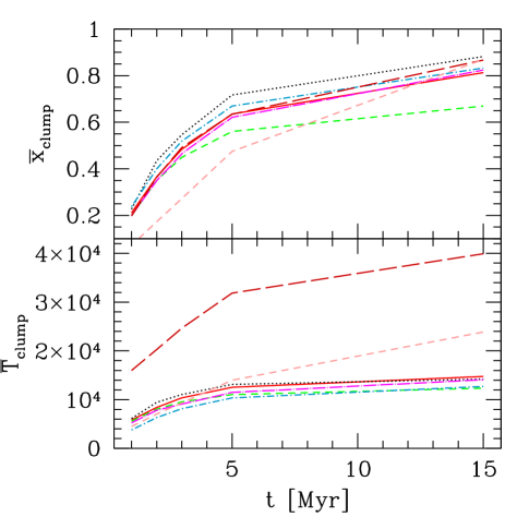
Figure 26: Test 3 (I-front trapping in dense clump): The evolution of the ionized fraction (top) and the mean temperature (bottom) inside the dense clump.

These observations are confirmed by the evolution of the mean ionized fraction and the mean temperature inside the clump shown in Figure 26. All codes agree very well on the evolution of the mean ionized fraction, except for CRASH, which finds about $\sim 25\%$ lower final ionized fraction, and for FLASH-HC, which early-on finds a lower ionized fraction, but catches up with the majority of the codes as the I-front becomes trapped. In terms of mean temperature, Coral, and to a lesser extent FLASH-HC find higher mean temperature due to the overheating of some cells mentioned above.

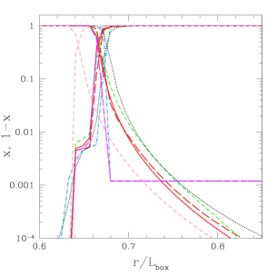
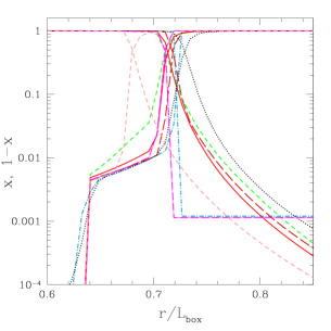
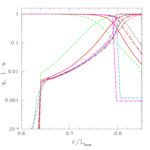
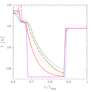
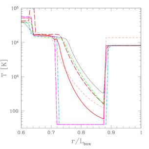
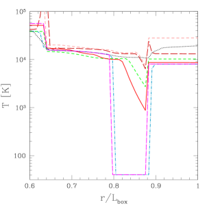
Figure 27: Test 3 (I-front trapping in dense clump): Line cuts of the ionized and neutral fraction along the axis of symmetry through the center of the clump at times $t=1$ Myr, 3 Myr and 15 Myr.

Figure 28: Test 3 (I-front trapping in dense clump): Line cuts of the temperature along the axis of symmetry through the center of the clump at times $t=1$ Myr, 3 Myr and 15 Myr.

In Figure 28 we show the ionized and neutral fraction profiles along the axis of symmetry at three stages of the evolution - early ($t=1$ Myr), during the slow-down due to recombinations ($t=3$ Myr, about one recombination time in the clump) and late ($t=15$ Myr). Only the region inside and around the clump is plotted in order to show details. In the pre-ionization, spectrum-hardening zone ahead of the main I-front all profiles agree fairly well at all times, except that the IFT profiles have a sharp I-front and no hardening by definition, and the FTTE current method appears to produce no hardening, either. Otherwise, these two codes agree well with the others in the post-front region. Some differences emerge in the position of the I-front (defined as the point of 50% ionized fraction) and the neutral fraction profiles behind the I-front. During the initial, fast propagation phase of the front all codes agree on its position. However, CRASH and, to a lesser extent, FLASH-HC both find consistently higher neutral fractions in the ionized part of the clump than the rest of the codes. As a consequence, they show that the I-front is trapped closer to the surface of the dense clump. The reason for this can be seen in the corresponding temperature profiles (Figure 29). Both CRASH and FLASH-HC obtain a slightly lower temperature for the dense ionized gas, resulting in a higher recombination rate there. The RSPH and IFT results show some diffusion at the source-side clump boundary (at $r/L_{\rm box}\sim 0.64$), resulting in a less sharp transition there, regardless of the sharp discontinuity of the gas density. The temperatures in the post-front fraction of the clump otherwise agree quite well, with the exception of the first cells on the source side, where Coral finds very high temperatures, as was already mentioned. In the pre-front region the temperature profile results also agree fairly well. Only IFT and FTTE differ there, again producing a very sharp I-front. $C^{2}$-Ray finds a bit less pre-heating in this region due to its single frequency bin method. Until $t=3$ Myr all results except the FLASH-HC one agree that the shadow region right behind the clump is completely shielded and remains at the initial temperature (8,000 K). At the final time, however, more differences emerge. At this time only IFT and FTTE still find no pre-heating, and $C^{2}$-Ray and CRASH find only little heating of the shadow. The Coral, RSPH and FLASH-HC results all find significant pre-heating, albeit at different levels. RSPH is the only code that at the final time finds no partially shielded gas at the back of the clump, the presence of which is indicated by the temperature dip at $r/L_{\rm box}\sim 0.88$ for all the other results.

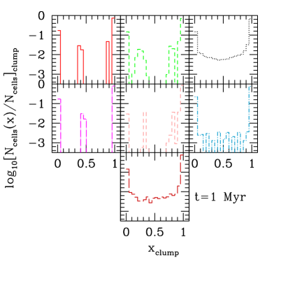
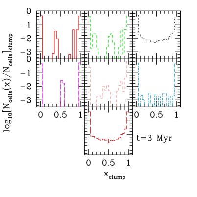
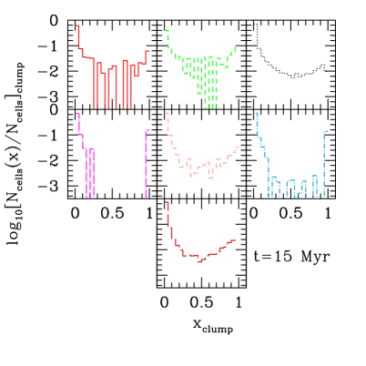
Figure 29: Test 3 (I-front trapping in dense clump): Histograms of the ionized fraction inside the clump at times $t=1$, 3 and 15 Myrs.

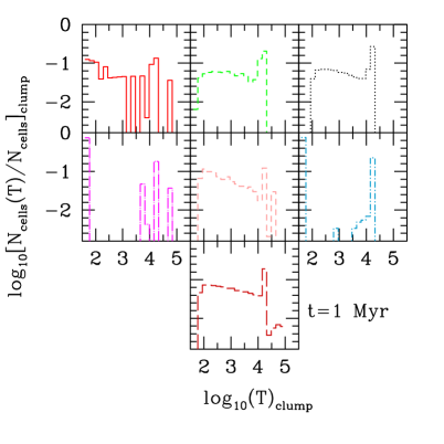
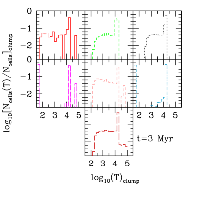
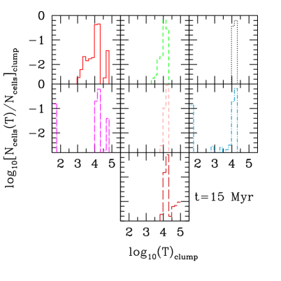
Figure 30: Test 3 (I-front trapping in dense clump): Histograms of the temperature inside the clump at times $t=1$, 3 and 15 Myrs.

The final results we show for this test are histograms of the fraction of cells inside the clump with a given ionized fraction (Figure 29) and with a given temperature (Figure 30) at the same three evolutionary stages discussed above. These histograms reflect the differences in the thickness and the internal structure of the I-fronts inside the clump. During the initial fast propagation and the slow-down phases the RSPH and Coral codes consistently find somewhat thicker I-front transitions than the other codes. The results of $C^{2}$-Ray, CRASH and FLASH-HC start with the front somewhat thinner than the ones for RSPH and Coral, but the distribution changes as the I-front gets trapped. At the final time, the ionized fraction distributions are very similar, with only the one for CRASH being slightly thicker. Finally, FTTE and IFT find significantly thinner front transitions and significant self-shielded gas fractions, as was noted before. The corresponding temperature distributions all show a strong peak at a similar temperature, a few tens of thousands of degrees, typical for gas heated by photoionization. This temperature is well above $10^{4}$ K because of the hot black-body spectrum of the source. At temperatures lower than this peak value, which largely correspond to the pre-heated zone ahead of the I-front, there again is broad agreement, apart from the FTTE and IFT codes which have a sharp front and little pre-heating. At the high-temperature end of the distribution $C^{2}$-Ray, FTTE, FLASH-HC and Coral diverge from the rest, by finding a small fraction of very hot cells, while the majority of codes find essentially no cells hotter than the distribution peak. It should be noted, however, that the fraction of these cells is only 0.1-1% of the total.

3.5 Test 4: Multiple sources in a cosmological density field

Test 4 involves the propagation of I-fronts from multiple sources in a static cosmological density field. The initial condition is provided by a time-slice (at redshift $z=9$) from a cosmological N-body and gas-dynamic simulation performed using the cosmological PM+TVD code by D. Ryu (Ryu et al. 1993). The simulation box size is $0.5\,h^{-1}$ comoving Mpc, the resolution is $128^{3}$ cells, $2\times 64^{3}$ particles. The halos in the simulation box were found using friends-of-friends halo finder with linking length of 0.25. For simplicity the initial temperature is fixed at $T=100$ K everywhere. The ionizing sources are chosen so as to correspond to the 16 most massive halos in the box. We assume that these have a black-body spectrum with effective temperature $T_{\rm eff}=10^{5}$ K. The ionizing photon production rate for each source is constant and is assigned assuming that each source lives $t_{s}=3$ Myr and emits $f_{\gamma}=250$ ionizing photons per atom during its lifetime, hence

$$\dot{N}_{\gamma}=f_{\gamma}\frac{M\Omega_{b}}{\Omega_{0}m_{p}t_{s}},$$ (13)

where $M$ is the total halo mass, $\Omega_{0}=0.27$, $\Omega_{b}=0.043$, $h=0.7$.

For simplicity all sources are assumed to switch on at the same time. The boundary conditions are transmissive (i.e. photons leaving the computational box are lost, rather than coming back in as in periodic boundary conditions). The evolution time is $t=0.4$ Myr.

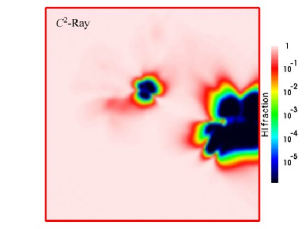
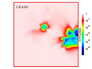
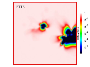
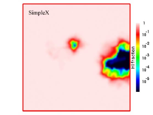
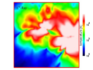
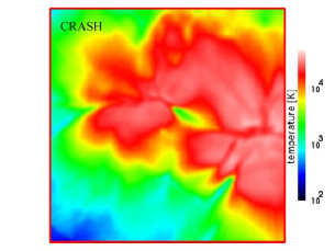
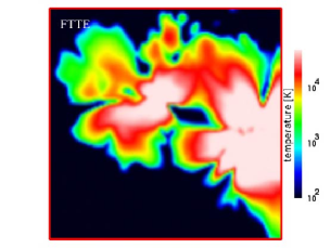
Figure 31: Test 4 (reionization of a cosmological density field): Images of the H I fraction, cut through the simulation volume at coordinate $z=z_{\rm box}/2$ and time $t=0.05$ Myr for $C^{2}$-Ray (left), CRASH (middle), FTTE (right), and SimpleX (bottom). The black-body spectrum has an effective temperature $T_{\rm eff}=10^{5}$ K.

Figure 32: Test 4 (reionization of a cosmological density field): Images of the temperature, cut through the simulation volume at coordinate $z=z_{\rm box}/2$ and time $t=0.05$ Myr for $C^{2}$-Ray (left), CRASH (middle), and FTTE (right). The black-body spectrum has an effective temperature $T_{\rm eff}=10^{5}$ K.

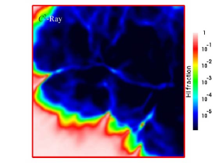
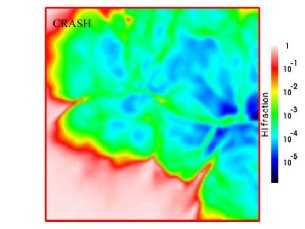
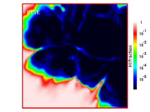
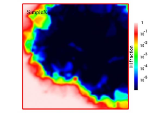
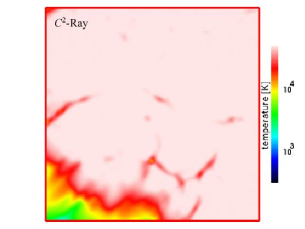
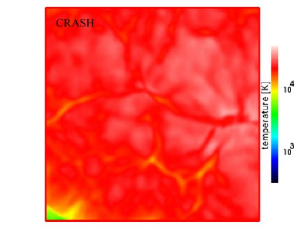
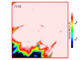
Figure 33: Test 4 (reionization of a cosmological density field): Images of the H I fraction, cut through the simulation volume at coordinate $z=z_{\rm box}/2$ and time $t=0.2$ Myr for $C^{2}$-Ray (left), CRASH (middle), FTTE (right), and SimpleX (bottom). The black-body spectrum has an effective temperature $T_{\rm eff}=10^{5}$ K.

Figure 34: Test 4 (reionization of a cosmological density field): Images of the temperature, cut through the simulation volume at coordinate $z=z_{\rm box}/2$ and time $t=0.2$ Myr for $C^{2}$-Ray (left), CRASH (middle), and FTTE (right). The black-body spectrum has an effective temperature $T_{\rm eff}=10^{5}$ K.

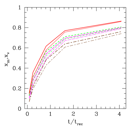
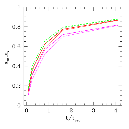
Figure 35: Test 4 (reionization of a cosmological density field): The evolution of the volume- and mass-weighted ionized fractions, $x_{v}$ (thin lines) and $x_{m}$ (thick lines), for a black-body source spectra with $T_{\rm eff}=10^{5}$ K (left) and $T_{\rm eff}=3\times 10^{4}$ K (right).

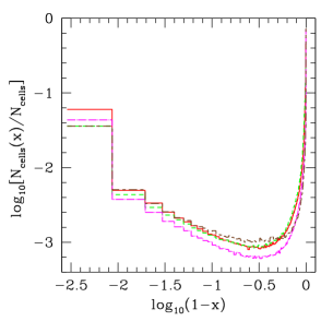
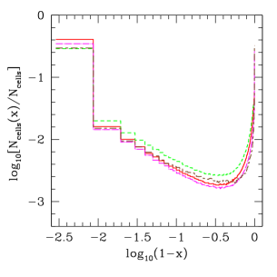
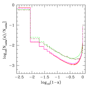
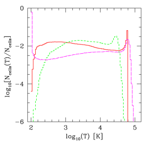
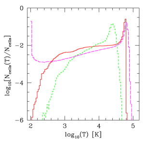
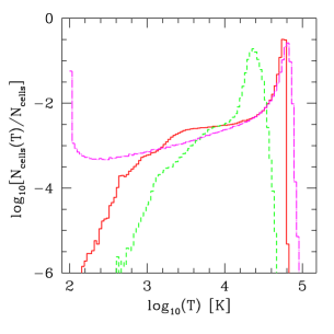
Figure 36: Test 4 (reionization of a cosmological density field): Histograms of the neutral fraction at times $t=0.05$, 0.2 and 0.4 Myrs for a black-body source spectrum with $T_{\rm eff}=10^{5}$ K.

Figure 37: Test 4 (reionization of a cosmological density field): Histograms of the temperature at times $t=0.05$, 0.2 and 0.4 Myrs for a black-body source spectrum with $T_{\rm eff}=10^{5}$ K.

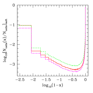
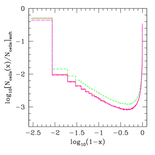
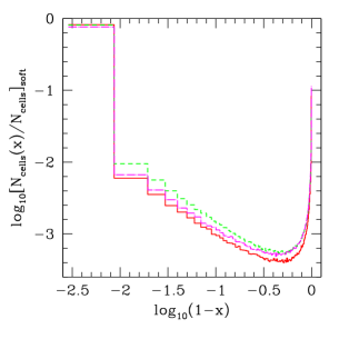
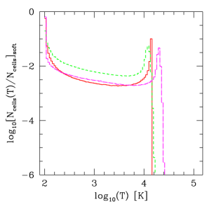
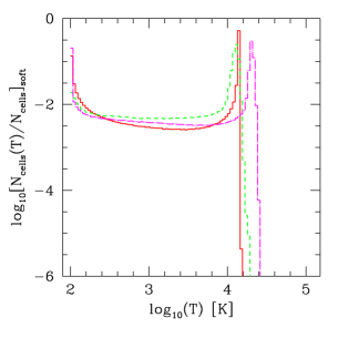
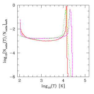
Figure 38: Test 4 (reionization of a cosmological density field): Histograms of the ionized fraction at times $t=0.05$, 0.2 and 0.4 Myrs for a black-body source spectrum with $T_{\rm eff}=3\times 10^{4}$ K.

Figure 39: Test 4 (reionization of a cosmological density field): Histograms of the temperature at times $t=0.05$, 0.2 and 0.4 Myrs for a black-body source spectrum with $T_{\rm eff}=3\times 10^{4}$ K.

In Figure 32 we show slices of the H I fraction cut through the simulation box at coordinate $z=z_{\rm box}/2$ and time $t=0.05$ Myr, and in Figure 32 we show the corresponding temperature distributions the same time. SimpleX does not appear in the temperature maps since currently the code does not follow the temperature evolution self-consistently, but instead assumes a constant temperature. In Figures 34 and 34 we show the same as above but at time $t=0.2$ Myr. Some discrepancies are already evident from a visual inspection, which shows somewhat different morphologies, but still general agreement. In Figure 35 (left panel) we present the temporal evolution of the volume- (thin lines) and mass- (thick lines) weighted ionized fractions. While CRASH and FTTE find comparable ionized fractions, $C^{2}$-Ray and SimpleX produce slightly higher and lower values, respectively. The lower value in SimpleX is obtained as a consequence of the temperature being fixed to $10^{4}$ K, which is a little lower than that obtained by the other codes, resulting in a higher recombination rate.

The finer sampling in CRASH of the high energy tail of the spectrum allows a higher resolution of its hardening. As the total energy is distributed differently from the other codes (more energy is in the hard photons), this results in less ionization/heating closer to the sources and more ionization/heating further away and a lower mean ionized fraction.

In Figures 37 and 37 we show histograms of the ionized fraction and the temperature at times $t=0.05$, 0.2 and 0.4 Myr are shown. While $C^{2}$-Ray and FTTE agree quite well, especially at later times, CRASH, as explained above, produces a thicker I-front transitions. The thickness of the I-front as found by SimpleX appears to oscillate with time, initially starting thick, then becoming thinner, and thick again towards the end of the simulation. This might have been caused by the interpolation of its unstructured grid to the regular grid required for the results. In terms of temperature, CRASH finds a systematically lower peak ($\sim 1.6\times 10^{4}$ K compared to $\sim 6.3\times 10^{4}$ K for $C^{2}$-Ray and FTTE, which agree well there) inside the ionized regions and a higher value in the lower density regions. This is once again due to the spectrum hardening effects discussed above. The peak produced by FTTE at very low temperatures arises because of the lack of spectrum hardening and sharp I-fronts consistently produced by this code, in which case no photons propagate ahead of the I-front and thus the gas away from the sources remains cold and neutral.

To understand whether the differences discussed above can be in fact attributed to photon hardening and the different treatment of the high energy tail of the spectrum, we have repeated the same simulations with a softer black-body spectrum with effective temperature $T_{\rm eff}=3\times 10^{4}$ K, in which case the spectrum hardening and I-front spreading should be minimized. We note that this part was not done by the SimpleX code since currently it does not treat different spectra. Our results are shown in Figures 35 (right panel),  39 and 39. The averaged ionized fraction produced by $C^{2}$-Ray and CRASH now have a much better agreement, as far fewer hard photons are present. However, FTTE still produces a lower value, although by only $\sim 5$%. CRASH still obtains a somewhat thicker ionizing front, due to the inherent adopted method, but the agreement is now better, especially at later times, as high energy photons are not present in this case. This is even more evident from an analysis of the temperature behaviour, where the agreement between $C^{2}$-Ray and CRASH is now very good at all times, while FTTE consistently finds higher temperatures inside the ionized regions. These higher temperatures seem to self-contradict the lower ionized fractions found by this code, while the recombination rate used by this code is consistent with the others, indicating a possible (modest) problem with photon conservation.

4 Summary and Conclusions

We have presented a detailed comparison of a large set of cosmological radiative transfer methods on several common tests. The participating codes represent the full variety of existing methods, multiple ray-tracing and one moment method, which solve the radiative transfer on regular, adaptive or unstructured grids, even with no grid at all, but instead using particles to represent the density field. The comparison is a collaborative project involving most of the cosmological RT community. The results from this comparison will be publicly available for testing of future codes during their development.

We began by comparing our basic physics, like chemistry, cooling rates and photoionization cross-sections, which came from a variety of sources, and evaluated the effects these have on the propagation of I-fronts. We concluded that even quite approximate rates generally result in relatively modest divergences in the results. The discrepancies were limited to $\sim 5-6\%$ in I-front position but were somewhat larger in velocity and the internal structure of the H II region (but never exceeding 20-40%, and usually much smaller).

Then, we turned to some simple, but instructive and cosmologically-interesting problems which tested the different aspects encountered in realistic applications. In summary, the results showed that at fixed temperature and for monochromatic ionizing spectrum all of these methods track I-fronts well, to within a few per cent accuracy. There are some differences in the inherent thickness (due to finite mean free path) and the internal structure of the I-fronts, related to some intrinsic diffusivity of some of the methods.

Somewhat greater differences emerge when the temperature is allowed to vary, although even in this case the agreement is very good, typically within 10-20% in the ionized fraction. Other variations between the results are due to the variety of multi-frequency radiative transfer methods and consequent spectrum hardening and pre-heating ahead of the I-fronts. Some of the algorithms consistently find quite sharp I-fronts, with little spectrum hardening and pre-heating, while the majority of the codes handle these features more precisely and in reasonable agreement among themselves.

We conclude that the various approximations employed by the different methods perform quite well and generally produce consistent and reliable results. There are, however, certain differences between the available methods and the most appropriate method for any particular problem would vary. Therefore, the code employed should be chosen with care depending on the specific questions whose answer is sought. For example, for problems in which the I-front structure is not resolved (due to coarse simulation resolution compared to the characteristic front width), most methods considered here should perform well and the main criterion should be their numerical efficiency. On the other hand, in problems where the I-front width and spectral hardening matters significantly, attention should be paid to the accurate multi-frequency treatment and the energy equation.

References

- Abel et al. (1997) Abel T., Anninos P., Zhang Y., Norman M. L., 1997, New Astronomy, 2, 181
- Abel & Wandelt (2002) Abel T., Wandelt B. D., 2002, MNRAS, 330, L53
- Aggarwal (1983) Aggarwal K. M., 1983, MNRAS, 202, 15P
- Aldrovandi & Pequignot (1973) Aldrovandi S. M. V., Pequignot D., 1973, A.&A, 25, 137
- Alvarez et al. (2005) Alvarez M. A., Bromm V., Shapiro P. R., 2005, ArXiv Astrophysics e-prints (astro-ph/0507684)
- Anninos et al. (1997) Anninos P., Zhang Y., Abel T., Norman M. L., 1997, New Astronomy, 2, 209
- Black (1981) Black J. H., 1981, MNRAS, 197, 553
- Burgess & Seaton (1960) Burgess A., Seaton M. J., 1960, MNRAS, 121, 471
- Cen (1992) Cen R., 1992, ApJS, 78, 341
- Ciardi & Ferrara (2005) Ciardi B., Ferrara A., 2005, Space Science Reviews, 116, 625
- Ciardi et al. (2001) Ciardi B., Ferrara A., Marri S., Raimondo G., 2001, MNRAS, 324, 381
- Cox (1970) Cox D. P., 1970, Ph.D. Thesis
- Frank & Mellema (1994) Frank A., Mellema G., 1994, A.&A, 289, 937
- Fryxell et al. (2000) Fryxell B., Olson K., Ricker P., Timmes F. X., Zingale M., Lamb D. Q., MacNeice P., Rosner R., Truran J. W., Tufo H., 2000, ApJS, 131, 273
- Fukugita & Kawasaki (1994) Fukugita M., Kawasaki M., 1994, MNRAS, 269, 563
- Górski et al. (2002) Górski K. M., Banday A. J., Hivon E., Wandelt B. D., 2002, in Astronomical Data Analysis Software and Systems XI, ASP Conference Series, Vol. 281,, Bohlender D. A., Durand D., Handley T. H., eds., p. 107
- Galli & Palla (1998) Galli D., Palla F., 1998, A.&A, 335, 403
- Gnedin & Abel (2001) Gnedin N. Y., Abel T., 2001, New Astronomy, 6, 437
- Górski et al. (2005) Górski K. M., Hivon E., Banday A. J., Wandelt B. D., Hansen F. K., Reinecke M., Bartelmann M., 2005, ApJ, 622, 759
- Haiman et al. (1996) Haiman Z., Thoul A. A., Loeb A., 1996, ApJ, 464, 523
- Heinemann et al. (2005) Heinemann T., Dobler W., Nordlund A., Brandenburg A., 2005, ArXiv Astrophysics e-prints (astro-ph/0503510)
- Hui & Gnedin (1997) Hui L., Gnedin N. Y., 1997, MNRAS, 292, 27
- Hummer (1994) Hummer D. G., 1994, MNRAS, 268, 109
- Hummer & Storey (1998) Hummer D. G., Storey P. J., 1998, MNRAS, 297, 1073
- Iliev et al. (2005a) Iliev I. T., Hirashita H., Ferrara A., 2005a, ArXiv Astrophysics e-prints (astro-ph/0509261)
- Iliev et al. (2005b) Iliev I. T., Mellema G., Pen U. L., Merz H., Shapiro P. R., Alvarez M. A., 2005b, submitted to MNRAS, (astro-ph/0512187)
- Iliev et al. (2005c) Iliev I. T., Shapiro P. R., Raga A. C., 2005c, MNRAS, 361, 405
- Janev et al. (1987) Janev R. K., Langer W. D., Evans K., 1987, Elementary processes in Hydrogen-Helium plasmas - Cross sections and reaction rate coefficients. Springer Series on Atoms and Plasmas, Berlin: Springer, 1987
- Lang (1974) Lang K. R., 1974, Astrophysical formulae: A compendium for the physicist and astrophysicist. New York, Springer-Verlag New York, Inc., 1974. 760 p.
- Maselli & Ferrara (2005) Maselli A., Ferrara A., 2005, ArXiv Astrophysics e-prints (astro-ph/0510258)
- Maselli et al. (2003) Maselli A., Ferrara A., Ciardi B., 2003, MNRAS, 345, 379
- Mellema et al. (2005) Mellema G., Arthur S. J., Henney W. J., Iliev I. T., Shapiro P. R., 2005, ArXiv Astrophysics e-prints (astro-ph/0512554)
- Mellema et al. (2006a) Mellema G., Iliev I. T., Alvarez M. A., Shapiro P. R., 2006a, New Astronomy, 11, 374
- Mellema et al. (2006b) Mellema G., Iliev I. T., Pen U. L., Shapiro P. R., 2006b, in preparation
- Mellema & Lundqvist (2002) Mellema G., Lundqvist P., 2002, A.&A, 394, 901
- Mellema et al. (1998) Mellema G., Raga A. C., Canto J., Lundqvist P., Balick B., Steffen W., Noriega-Crespo A., 1998, A.&A, 331, 335
- Nakamoto et al. (2001) Nakamoto T., Umemura M., Susa H., 2001, MNRAS, 321, 593
- Osterbrock (1974) Osterbrock D. E., 1974, Astrophysics of gaseous nebulae. W. H. Freeman and Co., 1974. 263 p.
- Osterbrock (1989) —, 1989, Astrophysics of gaseous nebulae and active galactic nuclei. University Science Books, 1989, 422 p.
- Peebles (1971) Peebles P. J. E., 1971, Physical cosmology. Princeton Series in Physics, Princeton, N.J.: Princeton University Press, 1971
- Peebles (1993) —, 1993, Principles of physical cosmology. Princeton Series in Physics, Princeton, NJ: Princeton University Press, —c1993
- Raga et al. (1997) Raga A. C., Mellema G., Lundqvist P., 1997, ApJS, 109, 517
- Razoumov & Cardall (2005) Razoumov A. O., Cardall C. Y., 2005, MNRAS, 362, 1413
- Razoumov et al. (2002) Razoumov A. O., Norman M. L., Abel T., Scott D., 2002, ApJ, 572, 695
- Rijkhorst (2005) Rijkhorst E.-J., 2005, Ph.D. Thesis
- Rijkhorst et al. (2006) Rijkhorst E.-J., Plewa T., Dubey A., Mellema G., 2006, A.&A(submitted)
- Ritzerveld (2005) Ritzerveld J., 2005, A.&A, 439, L23
- Ritzerveld et al. (2003) Ritzerveld J., Icke V., Rijkhorst E.-J., 2003, ArXiv Astrophysics e-prints (astro-ph/0312301)
- Ryu et al. (1993) Ryu D., Ostriker J. P., Kang H., Cen R., 1993, ApJ, 414, 1
- Shapiro et al. (2005) Shapiro P. R., Iliev I. T., Alvarez M. A., Scannapieco E., 2005, ApJ, submitted (astro-ph/0507677)
- Shapiro et al. (2004) Shapiro P. R., Iliev I. T., Raga A. C., 2004, MNRAS, 348, 753
- Shapiro & Kang (1987) Shapiro P. R., Kang H., 1987, ApJ, 318, 32
- Sherman (1979) Sherman R. D., 1979, ApJ, 232, 1
- Spitzer (1978) Spitzer L., 1978, Physical processes in the interstellar medium. New York Wiley-Interscience, 1978
- Springel (2005) Springel V., 2005, MNRAS, 364, 1105
- Steinmetz & Mueller (1993) Steinmetz M., Mueller E., 1993, A.&A, 268, 391
- Stone & Norman (1992) Stone J. M., Norman M. L., 1992, ApJS, 80, 753
- Strömgren (1939) Strömgren B., 1939, ApJ, 89, 526
- Susa (2006) Susa H., 2006, PASJ, accepted (astro-ph/0601642)
- Susa & Kitayama (2000) Susa H., Kitayama T., 2000, MNRAS, 317, 175
- Susa & Umemura (2004) Susa H., Umemura M., 2004, ApJ, 600, 1
- Tenorio-Tagle et al. (1986) Tenorio-Tagle G., Bodenheimer P., Lin D. N. C., Noriega-Crespo A., 1986, MNRAS, 221, 635
- Thacker et al. (2000) Thacker R. J., Tittley E. R., Pearce F. R., Couchman H. M. P., Thomas P. A., 2000, MNRAS, 319, 619
- Umemura (1993) Umemura M., 1993, ApJ, 406, 361
- Verner et al. (1996) Verner D. A., Ferland G. J., Korista K. T., Yakovlev D. G., 1996, ApJ, 465, 487
- Voronov (1997) Voronov G. S., 1997, Atomic Data and Nuclear Data Tables, 65, 1
- Whalen & Norman (2006) Whalen D., Norman M. L., 2006, ApJS, 162, 281